A&A 490, 487-492 (2008)
DOI: 10.1051/0004-6361:200809710
Z. Osmanov
E. Kharadze Georgian National Astrophysical Observatory, Kazbegi str. 2a, 0106 Tbilisi, Georgia
Received 4 March 2008 / Accepted 10 June 2008
Abstract
Aims. We investigate the centrifugally driven curvature drift instability to study how field lines twist close to the light cylinder surface of an AGN, through which the free motion of AGN winds can be monitored.
Methods. By studying the dynamics of the relativistic MHD flow close to the light cylinder surface, we derive and solve analytically the dispersion relation of the instability by applying a single particle approach based on the centrifugal acceleration.
Results. Considering the typical values of AGN winds, it is shown that the timescale of the curvature drift instability is far less than the accretion process timescale, indicating that the present instability is very efficient and might strongly influence processes in AGN plasmas.
Key words: instabilities - magnetohydrodynamics (MHD) - plasmas - galaxies: active - galaxies: nuclei - acceleration of particles
For studying AGN winds the fundamental problem relates to the understanding of a question: how the plasma goes through the Light Cylinder Surface LCS, which is the hypothetical zone where the linear velocity of rotation equals the speed of light. An innermost region of AGNs is characterized by the rotational motion, and it is obvious that this type of motion must affect the plasma dynamics. According to the standard model, the magnetic field due to the frozen-in condition generates plasmas, which consequently flow in the direction of and co-rotate with the field lines. This implies that the plasma particles, which move along quasi-straight magnetic field lines in the nearby area of the LCS, must reach the speed of light. On the other hand, no physical system can maintain such a motion and a certain twisting process of the magnetic field lines must operate on the LCS. In generalizing the work (Machabeli & Rogava 1994), Rogava et al. (2003) considered curved trajectories and studied the dynamics of a single particle moving along a rotating, curved channel. If the trajectories are given by the Archimedes spiral, then the particles can cross the LCS avoiding the light cylinder problem. An additional step in this investigation is to identify the appropriate mechanism that provides the twisting of the magnetic field lines, giving rise to the shape of the Archimedes spiral, and in turn insures the dynamics is force-free.
In the context of the force-free regime, the light cylinder problem has been studied numerically for pulsars. The investigation developed in Spitkovsky & Arons (2002) and Spitkovsky (2004) has shown that the plasma can travel through the LCS. This work was based on a current generated by the electric drift (Blandford 2002), which vanished for quasi-neutral plasmas and could not contribute to the dynamics of astrophysical flows, since it had almost equal numbers of positive and negative charges.
Since the innermost region of AGNs rotates, the role of the
Centrifugal Force (CF) appears interesting to the study of the
relativistic plasma motion. The centrifugally driven outflows have
been extensively studied. The study of Blandford & Payne (1982) deserves
particular attention because these authors discused the possibility
that the energy and angular momentum originated in the accretion
disk, emphasizing the role of the centrifugal acceleration in this
process. Gangadhara & Lesch (1997) considered the CF in the context of the
non-thermal radiation from the spinning AGNs. Generalizing the work
of Gangadhara & Lesch it was shown (Osmanov et al. 2007;
Rieger & Aharonian 2008), that due to the centrifugal acceleration, electrons
gain very high energies with Lorentz factors up to
![]() .
This implies that the energy budget in the AGN winds is very
high and if one finds a mechanism for the conversion of at least a
small fraction of this energy into a variety of instabilities, there
may be interesting consequences for the physics of AGN outflows.
.
This implies that the energy budget in the AGN winds is very
high and if one finds a mechanism for the conversion of at least a
small fraction of this energy into a variety of instabilities, there
may be interesting consequences for the physics of AGN outflows.
The centrifugal force may drive different types of instabilities. Obviously, the CF that acts on a moving particle changes with time and, in the context of instabilities, plays a role in determining this parameter. Consequently, the corresponding instability is called the parametric instability.
The centrifugally driven parametric instability was first introduced by Machabeli et al. (2005) for the Crab pulsar magnetosphere. We argued that the centrifugal force may cause the separation of charges, leading to the creation of an unstable electrostatic field. Estimating the linear growth rate, it was shown that the instability was extremely efficient. The method developed by Machabeli et al. (2005) was applied to AGN jets (Osmanov 2008) in studying the stability problem of the rotation-induced electrostatic instability and for understanding how efficient is the centrifugal acceleration in this process. Another kind of the instability which might be induced by the CF is the so called Curvature Drift Instability (CDI). Even if the field lines have initially a very small curvature, this curvature might cause a drifting process of plasma, which priduces to the CDI. Osmanov et al. (2008a) considered the two-component relativistic plasma in studying the role of the centrifugal acceleration in the curvature drift instability for pulsar magnetospheres. The investigation demonstrated that the growth rate was higher than pulsar spin-down rates by many orders of magnitude, which implied that the CDI was highly efficient. The curvature drift current produces the toroidal component of the magnetic field, which due to the efficient unstable character of the process amplifies rapidly, changing the overall configuration of the magnetic field. This leads to the transformation of field lines into the shape of the Archimedes spiral, when the motion of the particles switches to the so-called force-free regime (Osmanov et al. 2008b) and the plasma goes through the LCS.
To investigate the twisting process of magnetic field lines due to the CDI, we apply the method developed by Osmanov et al. (2008a) and Osmanov et al. (2008b) to AGN winds.
The paper is arranged as follows. In Sect. 2, we introduce the curvature drift waves and derive the dispersion relation. In Sect. 3, the results for typical AGNs are presented and, in Sect. 4, we summarize our results.
We begin our investigation by considering the two-component plasma
consisting of the relativistic electrons with the Lorentz factor
![]() (Osmanov et al. 2007; Rieger & Aharonian 2008) and the
bulk component (protons) with
(Osmanov et al. 2007; Rieger & Aharonian 2008) and the
bulk component (protons) with
![]() .
Since we are
interested in the twisting process, we suppose that initially the
field lines are almost rectilinear to study how this configuration
changes in time.
.
Since we are
interested in the twisting process, we suppose that initially the
field lines are almost rectilinear to study how this configuration
changes in time.
We start by considering the Euler equation governing the dynamics of
plasma particles, co-rotating with the straight magnetic-field
lines. By applying the method developed by Chedia et al. (1996), owe can
show that the Euler equation assume the following form:
In the zeroth approximation, the plasma particles are affected only by the centrifugal force. Different species at different positions experience different CFs, which cause the separation of charges, leading to the creation of the additional electromagnetic field considered as the first order term in our equations.
The leading state is characterized by the frozen-in condition,
![]() ,
which reduces Eq. (1) into the following form (Machabeli & Rogava 1994):
,
which reduces Eq. (1) into the following form (Machabeli & Rogava 1994):
Since we assume that the magnetic field lines have initially a small curvature, the particles moving radially drift along the x axis (Osmanov et al. 2008a) (see Fig. 1). The afore mentioned drift of charges produces a corresponding current, which inevitably creates the toroidal magnetic field, changing the overall configuration of the field lines. Therefore, the aim of the present work is to study the role of the centrifugally induced curvature drift instability in the twisting process of the magnetic field lines. For this purpose, we linearize the system of equations Eqs. (1)-(3), perturbing all physical quantities around the leading state:
![\begin{figure}
\par {\includegraphics[angle=0,width=8cm,clip]{9710fig.ps} }
\end{figure}](/articles/aa/full/2008/41/aa09710-08/img62.gif) |
Figure 1:
Two orthonormal bases are
considered: i) cylindrical components of unit vectors, (
|
| Open with DEXTER | |
We express
![]() and
and
![]() in the following way:
in the following way:
![\begin{displaymath}\times
B_{r}\left(\omega+\Omega
\left(2[s-l]+n-p+\sigma\right...
...\alpha}}{\omega
+ \frac{k_xu_{\alpha}}{2}+\Omega (2s+n)}\right]\end{displaymath}](/articles/aa/full/2008/41/aa09710-08/img73.gif)
![\begin{displaymath}+\sum_{\alpha=e,b}\frac{\omega^2_{\alpha}k_xu_{\alpha}}{4\gam...
...omega
+ \frac{k_xu_{\alpha}}{2}+\Omega (2[s+\mu]+n)\right)^2 } \end{displaymath}](/articles/aa/full/2008/41/aa09710-08/img74.gif)
We consider the parameters
![]() erg/s,
erg/s,
![]() s-1,
s-1,
![]() ,
,
![]()
![]() cm-3 typical for AGN winds. Then, examining the
curvature drift waves with
cm-3 typical for AGN winds. Then, examining the
curvature drift waves with
![]() (
(
![]() is
the wave length), we can show that
is
the wave length), we can show that
![]() s
s
![]() ,
where, it is assumed that kx<0 and
,
where, it is assumed that kx<0 and
![]() ,
otherwise the frequency becomes negative. Therefore, all
terms with non-zero values of
,
otherwise the frequency becomes negative. Therefore, all
terms with non-zero values of
![]() and
and
![]() oscillate rapidly and do not contribute to the final
result. Consequently, the only terms that influence the solution of
Eq. (19) are the leading terms, the contribution of which
simplifies the equation (Osmanov et al. 2008a) (see Appendix B):
oscillate rapidly and do not contribute to the final
result. Consequently, the only terms that influence the solution of
Eq. (19) are the leading terms, the contribution of which
simplifies the equation (Osmanov et al. 2008a) (see Appendix B):
We investigate the efficiency of the CDI in AGN winds. The behaviour of the growth rate is considered in terms of the wavelength, the density of relativistic electrons, their Lorentz factors and the AGN bolometric luminosity.
In studying the behaviour of the instability as a function of the
wavelength, we examine the typical AGN parameters:
![]() ,
,
![]() s-1and
L = 1044 erg/s, where
s-1and
L = 1044 erg/s, where
![]() is the AGN mass,
is the AGN mass, ![]() is the solar mass and L is the bolometric luminosity of the AGN.
is the solar mass and L is the bolometric luminosity of the AGN.
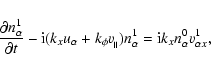
We consider Eq. (23) and plot the logarithm of the
instability timescale
![\begin{figure}
\par {\includegraphics[angle=0,width=8cm,clip]{9710lambda1.ps} }
\end{figure}](/articles/aa/full/2008/41/aa09710-08/img116.gif) |
Figure 2:
The dependence of logarithm of the instability timescale
on the normalized wave length. The set of parameters is
|
| Open with DEXTER | |
![\begin{figure}
\par {\includegraphics[angle=0,width=8cm,clip]{9710density1.ps} }
\end{figure}](/articles/aa/full/2008/41/aa09710-08/img117.gif) |
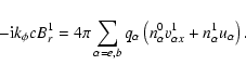
Figure 3:
The dependence of logarithm of the instability timescale
on the density normalized by the medium density. The set of parameters is
|
| Open with DEXTER | |
Since the CDI growth rate depends on the plasma frequency (see Eqs. (23), (22)), which is in turn a function of the
density, it is obvious that the instability timescale must be
influenced by the density of relativistic electrons in the AGN
winds. In Fig. 3 the plots of
![]() versus the AGN
wind density illustrate that the timescale is a continuously
decreasing function of
versus the AGN
wind density illustrate that the timescale is a continuously
decreasing function of
![]() .
The set of parameters is the
same as in Fig. 2, apart from
.
The set of parameters is the
same as in Fig. 2, apart from
![]() and
and
![]() .
Here,
.
Here,
![]() is normalized by the
intergalactic medium density,
is normalized by the
intergalactic medium density,
![]() .
As we see from
the figure,
.
As we see from
the figure, ![]() varies from
varies from ![]() 109 s (
109 s (
![]() ,
,
![]() )
to
)
to ![]() 106 s (
106 s (
![]() ,
,
![]() ).
).
![\begin{figure}
\par {\includegraphics[angle=0,width=8cm,clip]{9710gamma1.ps} }
\end{figure}](/articles/aa/full/2008/41/aa09710-08/img126.gif) |
Figure 4:
The dependence of logarithm of the instability time scale
on
|
| Open with DEXTER | |
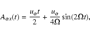
In Fig. 4, the plot of
![]() versus
versus
![]() is shown for different luminosities. The set of
parameters is the same as in Fig. 2 apart from the
continuous range of
is shown for different luminosities. The set of
parameters is the same as in Fig. 2 apart from the
continuous range of
![]() ,
some values of
the luminosity
,
some values of
the luminosity
![]() ,
and
,
and
![]() .
The figure shows the continuously decreasing behaviour of
the instability timescale, which is a natural consequence of the
fact that the more energetic electrons induce the curvature drift
instability more efficiently. From Eq. (12) it is clear
that the drift velocity is proportional to the Lorentz factor of the
particle, and hence the corresponding instability is more efficient,
producing the decrease in
.
The figure shows the continuously decreasing behaviour of
the instability timescale, which is a natural consequence of the
fact that the more energetic electrons induce the curvature drift
instability more efficiently. From Eq. (12) it is clear
that the drift velocity is proportional to the Lorentz factor of the
particle, and hence the corresponding instability is more efficient,
producing the decrease in
![]() .
As we see, the instability
timescale varies from
.
As we see, the instability
timescale varies from ![]() 1010 s (
1010 s (
![]() ,
,
![]() )
to
)
to ![]() 108 s (
108 s (
![]() ,
,
![]() ). On
the other hand, the plots for different luminosities illustrates
another property of
). On
the other hand, the plots for different luminosities illustrates
another property of ![]() :
by increasing the luminosity of the AGN,
the corresponding instability becomes less efficient.
:
by increasing the luminosity of the AGN,
the corresponding instability becomes less efficient.
To observe this particular feature more clearly, we consider how in
Fig. 5 the dependence of
![]() on
on
![]() is clearly
evident for different values of densities. From the plots, it is
seen that by increasing the luminosity, the timescale continuously
increases. This behaviour follows from the fact that the bigger the
luminosity, the larger the magnetic field (see Eq. (13))
and hence the lower the drift velocity, producing the less efficient
CDI shown in the figure. By considering larger values of densities,
the CDI becomes more efficient, which we explained already while
considering Fig. 3. For the afore mentioned area of
quantities (see Fig. 5), the timescale varies from
is clearly
evident for different values of densities. From the plots, it is
seen that by increasing the luminosity, the timescale continuously
increases. This behaviour follows from the fact that the bigger the
luminosity, the larger the magnetic field (see Eq. (13))
and hence the lower the drift velocity, producing the less efficient
CDI shown in the figure. By considering larger values of densities,
the CDI becomes more efficient, which we explained already while
considering Fig. 3. For the afore mentioned area of
quantities (see Fig. 5), the timescale varies from ![]() 107 s (
107 s (
![]() ,
,
![]() )
to
)
to ![]() 1010 s (
1010 s (
![]() ,
,
![]() ).
).
We observe from the present investigation that the instability
timescale varies in the following range:
![]() s.
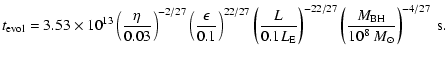
To specify how efficient the CDI is, it is pertinent to examine an
accretion process, estimate its corresponding evolution timescale,
and compare this value with that of the CDI.
s.
To specify how efficient the CDI is, it is pertinent to examine an
accretion process, estimate its corresponding evolution timescale,
and compare this value with that of the CDI.
![\begin{figure}
\par {\includegraphics[angle=0,width=8cm,clip]{9710luminosity1.ps} }
\end{figure}](/articles/aa/full/2008/41/aa09710-08/img133.gif) |
Figure 5:
The dependence of logarithm of the instability time scale
on
|
| Open with DEXTER | |
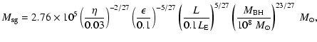
Considering the problem of fuelling AGNs, King & Pringle
(2007) showed that the self-gravitating mass in accretion flows
can be estimated by the following expression:
![\begin{figure}
\par {\includegraphics[angle=0,width=8.5cm,clip]{9710fig1.ps} }
\end{figure}](/articles/aa/full/2008/41/aa09710-08/img143.gif) |
Figure 6:
The behaviour of logarithm of the evolution timescale versus M9 and
|
| Open with DEXTER | |
In Fig. 6, we show the two-dimensional surface of logarithm
of the evolution timescale. The variables are in the following
range:
![]() and
and
![]() .
For plotting the figure, we took into account
that, according to the observations, AGN masses vary in the
following range:
.
For plotting the figure, we took into account
that, according to the observations, AGN masses vary in the
following range:
![]() (Nelson 2000). As is clear from Fig. 6,
(Nelson 2000). As is clear from Fig. 6,
![]() is a
continuously decreasing function of M9 and
is a
continuously decreasing function of M9 and
![]() .
The minimum
value of the evolution timescale (
.
The minimum
value of the evolution timescale (![]() 1012 s), when the
accretion process is extremely efficient corresponds to M9 = 1and
1012 s), when the
accretion process is extremely efficient corresponds to M9 = 1and
![]() ,
whereas the maximum value, approximately
,
whereas the maximum value, approximately ![]() 1015 s, corresponds to the following pair of variables
M9 =
0.001 and
1015 s, corresponds to the following pair of variables
M9 =
0.001 and
![]() .
.
To understand how efficient the curvature drift instability is, we
have to compare the corresponding timescale with the evolution
timescale. As has been found, depending on physically reasonable
parameters, ![]() varies in the range
varies in the range ![]() (106-1010) s,
whereas the sensible area of
(106-1010) s,
whereas the sensible area of
![]() is
is ![]() (1012-1015) s. Therefore, the instability timescale is less
than the evolution timescale of the accretion by many orders of
magnitude, which implies that the linear stage of the CDI is
extremely efficient.
(1012-1015) s. Therefore, the instability timescale is less
than the evolution timescale of the accretion by many orders of
magnitude, which implies that the linear stage of the CDI is
extremely efficient.
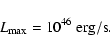
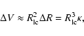
The twisting process of magnetic field lines requires a certain
amount of energy and it is natural to study the energy budget of
this process. For this reason we have to introduce the maximum of
the possible luminosity
![]() and compare this with
the ``luminosity'' corresponding to the reconstruction of the magnetic
field configuration
and compare this with
the ``luminosity'' corresponding to the reconstruction of the magnetic
field configuration
![]() ,
where
,
where
![]() is the variation in the magnetic
energy due to the curvature drift instability.
is the variation in the magnetic
energy due to the curvature drift instability.
![\begin{figure}
\par {\includegraphics[angle=0,width=8cm,clip]{9710energy1.ps} }
\end{figure}](/articles/aa/full/2008/41/aa09710-08/img151.gif) |
Figure 7:
The dependence of
|
| Open with DEXTER | |
We consider a AGN of the luminosity,
L = 1045 erg/s, then, by
applying Eq. (26) and taking into account that
![]() ,
we show that the accretion provides the following maximum
value:
,
we show that the accretion provides the following maximum
value:
We introduce the initial non-dimensional perturbation, ![]() ,
defined to be
,
defined to be
![]() ,
where by B0 we denote the
induction of the magnetic field in the leading state (see Eq. (31)). By considering the following set of parameters
,
where by B0 we denote the
induction of the magnetic field in the leading state (see Eq. (31)). By considering the following set of parameters
![]() ,
,
![]() ,
,
![]() cm-3,
cm-3,
![]() ,
,
![]() and
L = 1045 erg/s, we plot the behaviour of
and
L = 1045 erg/s, we plot the behaviour of
![]() versus the initial perturbation for the
characteristic timescale (
versus the initial perturbation for the
characteristic timescale (
![]() ). As we can see from Fig. 7,
). As we can see from Fig. 7,
![]() varies from
varies from ![]() 0 (
0 (
![]() )
to
)
to ![]()
![]() (
(
![]() ,
,
![]() ).
Therefore, the maximum luminosity, and therefore the total
luminosity budget, exceeds, by many orders of magnitude, the
magnetic luminosity required for the twisting of the field lines.
This means that only a tiny fraction of the total energy goes to the
sweepback, making this process feasible.
).
Therefore, the maximum luminosity, and therefore the total
luminosity budget, exceeds, by many orders of magnitude, the
magnetic luminosity required for the twisting of the field lines.
This means that only a tiny fraction of the total energy goes to the
sweepback, making this process feasible.
We summarize the principal steps and conclusions of our study to be:
The next limitation is related to the fact that the magnetic field lines were supposed to be quasi rectilinear, whereas in real astrophysical situations the field lines might be initially curved. This particular case also needs to be studied by generalizing the present model.
In this paper, the field lines located in the equatorial plane have been considered, although in realistic situations, the magnetic field lines also might be inclined with respect to the equatorial plane. Therefore, it is essential to examine this particular case as well and see how the efficiency of the CDI changes, when the field line's inclination with respect to the equatorial plane is taken into account.
Acknowledgements
I thank professor G. Machabeli for valuable discussions. The research was supported by the Georgian National Science Foundation grant GNSF/ST06/4-096.
![\begin{displaymath}
\frac{{\rm d}v}{{\rm d}t}=\frac{\Omega^2R}{1-
\frac{\Omega^...
...}\left[1-\frac{\Omega^2R^2}{c^2}-
\frac{2v^2}{c^2}\right]\cdot
\end{displaymath}](/articles/aa/full/2008/41/aa09710-08/img41.gif)
![\begin{displaymath}
\Psi^1(t,{\vec{r}})\propto\Psi^1(t)
\exp\left[{\rm i}\left({\vec{kr}} \right)\right] ,
\end{displaymath}](/articles/aa/full/2008/41/aa09710-08/img49.gif)


![\begin{displaymath}
\Gamma\approx \left[\sum_{\sigma,\mu = \pm
1}\sum_{s,l}\Xi_...
..._{-2(s +
\mu)}(h)J_l(g)J_{-2l+\sigma}(h)\right]^{\frac{1}{2}}.
\end{displaymath}](/articles/aa/full/2008/41/aa09710-08/img98.gif)