A&A 488, 113-116 (2008)
DOI: 10.1051/0004-6361:200810141
Supermassive black hole masses in type II active galactic nuclei with
polarimetric broad emission lines
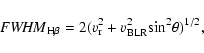
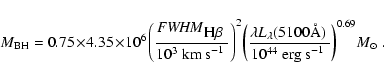
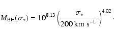
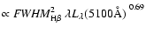
S.-Y. Zhang1 - W.-H. Bian1,2 - K.-L. Huang1
1 - Department of Physics and Institute of Theoretical
Physics, Nanjing Normal University, Nanjing 210097, PR China
2 -
Key Laboratory for Particle Astrophysics, Institute of High Energy
Physics, Chinese Academy of Sciences, Beijing 100039, PR China
Received 6 May 2008 / Accepted 10 June 2008
Abstract
Aims. Type II active galactic nuclei (AGNs) with polarimetric broad emission lines provided strong evidence for the orientation-based unified model for AGNs. We want to investigate whether the polarimetric broad emission lines in type II AGNs can be used to calculate their central supermassive black hole (SMBH) masses, like that for type I AGNs.
Methods. We collected 12 type II AGNs with polarimetric broad emission line widths from the literature, and calculated their central black hole masses from the polarimetric broad line widths and the isotropic [O III] luminosity. We also calculate the mass from stellar velocity dispersion,  ,
with the
,
with the
 relation.
Results. We find that: (1) the black hole masses derived from the polarimetric broad line width is on average larger than that from the
relation by about 0.6 dex; (2) if these type II AGNs follow a
relation, we find that the random velocity cannot be omitted and is comparable to the broad-line regions (BLRs) Keplerian velocity. It is consistent with the scenery of large outflow from the accretion disk suggested by Yong et al.
Key words: galaxies: quasars:
emission lines - galaxies: nuclei - black hole physics
The standard paradigm for active galactic nuclei (AGNs) posits an
accretion disk surrounding a central supermassive black hole (SMBH),
along with other components, such as the broad-line regions (BLRs),
narrow-line regions (NLRs), jet, and torus (e.g., Antonoucci 1993).
The black hole mass (
 )
is an important parameter for us to
understand the nuclear energy mechanics, the formation and evolution
of SMBH, and galaxies (e.g., Rees 1984; Tremaine et al. 2002).
)
is an important parameter for us to
understand the nuclear energy mechanics, the formation and evolution
of SMBH, and galaxies (e.g., Rees 1984; Tremaine et al. 2002).
In the past decade, one of the most important advances in the study
of AGNs is that the masses of SMBHs can be calculated by using the
width of the broad emission lines from BLRs (e.g.,
 ,
,
 ,
,
 ,
,
 )
by the reverberation mapping method and several
corresponding empirical relations (e.g., Kaspi et al. 2000; Bian &
Zhao 2004; Greene & Ho 2006). In the orientation-based unified
model for AGNs, the distinction between type I AGNs and type II AGNs
depends upon whether the central engine and BLRs are viewed directly
(type I) or are obscured by the circumnuclear torus (type II).
Because of the absence of broad emission lines in the spectrum of
type II AGNs, above methods for the mass calculation are only
applicable to type I AGNs. The SMBH mass in the center of type II
AGNs generally may be estimated by the
relation
(e.g., Kauffmann et al. 2003; Bian & Gu 2007).
)
by the reverberation mapping method and several
corresponding empirical relations (e.g., Kaspi et al. 2000; Bian &
Zhao 2004; Greene & Ho 2006). In the orientation-based unified
model for AGNs, the distinction between type I AGNs and type II AGNs
depends upon whether the central engine and BLRs are viewed directly
(type I) or are obscured by the circumnuclear torus (type II).
Because of the absence of broad emission lines in the spectrum of
type II AGNs, above methods for the mass calculation are only
applicable to type I AGNs. The SMBH mass in the center of type II
AGNs generally may be estimated by the
relation
(e.g., Kauffmann et al. 2003; Bian & Gu 2007).
With spectro-polarimetric observation, some type II AGNs show hidden
BLRs (HBLRs) and some do not (e.g., Antonucci  Miller 1985; Tran
1995). It is still not clear what kind of physical process is
related to the presence of HBLRs in type II AGNs (e.g., Bian & Gu
2007). We calculate the SMBH mass in type II AGNs with HBLRs by
using broad emission lines in their polarimetric spectrum as well as
the
relation. In Sect. 2, we briefly introduce our
sample. Section 3 introduces the methods to calculate the SMBH masses.
Section 4 is the data analysis. Our results and discussions are given
in Sect. 5. The last section is our conclusion. All of the
cosmological calculations in this paper assume
Miller 1985; Tran
1995). It is still not clear what kind of physical process is
related to the presence of HBLRs in type II AGNs (e.g., Bian & Gu
2007). We calculate the SMBH mass in type II AGNs with HBLRs by
using broad emission lines in their polarimetric spectrum as well as
the
relation. In Sect. 2, we briefly introduce our
sample. Section 3 introduces the methods to calculate the SMBH masses.
Section 4 is the data analysis. Our results and discussions are given
in Sect. 5. The last section is our conclusion. All of the
cosmological calculations in this paper assume
 Mpc-1,
 ,
,
 .
.
We collected a sample of 12 type II AGNs with HBLRs from the
literature, which provide us with the hidden broad line width (Table 1). In this sample, there are 8 type II AGNs with redshifts z<0.05(Tran 1995), the rest are in the redshift range 0.3<z<0.8, which
are from Zakamska et al. (2007).
For Mrk 3 and Mrk 348, Tran (1995) used a sixth- or seventh-order
polynomial to extract polarimetric broad line profiles for their
high s/N. For the remaining objects in Tran (1995), multiple
Gaussians are used to extract polarimetric broad line profiles for
measuring the full widths at half-maximum (FWHM). For four objects
in Zakamska et al. (2007), FWHM for polarimetric broad emission
lines are obtained through Gaussian fits. These polarimetric broad
emission lines are obvious because Zakamska et al. (2007) adopted a
sensitivity limit of about 100 Å in equivalent width for these
lines, which is larger than that for H line in the composite
quasar spectrum (46 Å; Vanden Berk et al. 2001).
line in the composite
quasar spectrum (46 Å; Vanden Berk et al. 2001).
Assuming that the gas in BLRs is virial in the gravitational field
of the central SMBH, we can calculate the SMBH masses with the
following formula (e.g., Kaspi et al. 2000; Kaspi et al. 2005):
 |
(1) |
where G is the gravitational constant, and
 is the
distance from BLRs clouds to the central black hole. This can be
calculated from the monochromatic luminosity at
is the
distance from BLRs clouds to the central black hole. This can be
calculated from the monochromatic luminosity at
 by
the empirical size-luminosity relation, that is (Kaspi et al. 2005):
by
the empirical size-luminosity relation, that is (Kaspi et al. 2005):
 |
(2) |
where
 is the BLRs virial velocity, which can be traced
by using FWHM of the broad
line (
is the BLRs virial velocity, which can be traced
by using FWHM of the broad
line (
 )
or
)
or
 line; that is:
 |
(3) |
where f is the scaling factor. If BLRs cloud is disk-like with an inclination of  (Wills
Browne 1986; Collin et al. 2006):
(Wills
Browne 1986; Collin et al. 2006):
 |
(4) |
where  is the random isotropic component. If assuming
 and the random orbits of clouds in BLRs, then f=0.75, i.e.,
 .
Therefore, the formula (1)
can be transformed into the following form:
.
Therefore, the formula (1)
can be transformed into the following form:
 |
(5) |
For type II AGNs, we could not obtain the intrinsic monochromatic
luminosity at 5100 Å from their spectrum because of torus
obscuration. The [O III] 5007 luminosity,
![$L_{\rm [O III]}$](/articles/aa/full/2008/34/aa10141-08/img33.gif) ,
coming from NLRs is not obscured and is isotropic. Kauffmann et al.
(2003) have shown that the extinction-corrected
,
coming from NLRs is not obscured and is isotropic. Kauffmann et al.
(2003) have shown that the extinction-corrected
![$L^{\rm cor}_{\rm [O
III]}$](/articles/aa/full/2008/34/aa10141-08/img34.gif) is a good indicator of AGN activity for type II AGNs. The
unobscured monochromatic luminosity at 5100 Å is calculated by the
following relation (e.g., Kaspi et al. 2000; Heckman et al. 2004;
Netzer & Trakhtenbrot 2007):
is a good indicator of AGN activity for type II AGNs. The
unobscured monochromatic luminosity at 5100 Å is calculated by the
following relation (e.g., Kaspi et al. 2000; Heckman et al. 2004;
Netzer & Trakhtenbrot 2007):
![\begin{displaymath}L_{\rm bol}=9 [\mbox{$\lambda L_{\lambda}(5100\AA)$\ }]=3500L^{\rm cor}_{[\rm O III]} .
\end{displaymath}](/articles/aa/full/2008/34/aa10141-08/img35.gif) |
(6) |
The second method for us to calculate the black hole masses is the
relationship to the stellar velocity dispersion ()
in
their host galaxies (Tremaine et al. 2002):
 |
(7) |
For 8 type II AGNs with redshifts z<0.05, we obtained their
stellar velocity dispersions from the literature (see Table 1). The
other 4 type II AGNs in the redshift range 0.3<z<0.5 are
selected from the spectroscopic database of SDSS, their host
galaxies light is too weak to directly measure the stellar velocity
dispersion, .
Because NLRs are primarily controlled by the
host gravitational potential,the FWHM of the core/narrow [O III]5007 line after removing the asymmetric blue wing can
be used to trace the stellar velocity dispersion for these 4 type II
AGNs (Nelson & Whittle 1996; Greene & Ho 2005):
![\begin{displaymath}\sigma_*= {\it FWHM}^{\rm core}_{\rm [O III]}/2.35 .
\end{displaymath}](/articles/aa/full/2008/34/aa10141-08/img37.gif) |
(8) |
For 4 type II AGNs with redshifts 0.3<z<0.5, we downloaded their
spectrum from the SDSS(the Sloan Dgital Sky Survey) spectroscopic
database and used following steps to do the SDSS spectral
measurements, which has been used for SDSS type I AGNs. (1) First,
we estimate the Galactic extinction in observed spectra by using the
extinction law of Cardelli et al. (1989, IR band) and
O'Donnell (1994, optical band), then the spectra are transformed into
the rest frame defined by the redshifts given in their FITS headers.
(2) The
 template is from NLS1 I ZW1 model, the Balmer
continuum are calculated following Grandi (1982). The best
subtraction of the
,
power-law and Balmer continuum is found
when
template is from NLS1 I ZW1 model, the Balmer
continuum are calculated following Grandi (1982). The best
subtraction of the
,
power-law and Balmer continuum is found
when  minimized in the fitting windows: 3550-3645,
4170-4260, 4430-4770, 5080-5550, 6050-6220, 6890-7010
minimized in the fitting windows: 3550-3645,
4170-4260, 4430-4770, 5080-5550, 6050-6220, 6890-7010  .
Since
they are the spectra of type II AGNs, the
line and Balmer
continuum could be neglected, the power-law continuum seems flat
(see a sample fit in the a panel of Fig. 1). (3) Two sets of
two-Gaussian are used to model [O III]
.
Since
they are the spectra of type II AGNs, the
line and Balmer
continuum could be neglected, the power-law continuum seems flat
(see a sample fit in the a panel of Fig. 1). (3) Two sets of
two-Gaussian are used to model [O III]
 lines. We take the same line width for each component, and fix the
flux ratio of [O III]4959 to [O III]5007 to be 1:3.
Two-Gaussian profile is used to model H
line. (see the b panel of
Fig. 1). From above spectral measurement, we obtain the FWHM of
the narrow/core [O III] line, as well as the total [O III] luminosity
(see Table 1).
lines. We take the same line width for each component, and fix the
flux ratio of [O III]4959 to [O III]5007 to be 1:3.
Two-Gaussian profile is used to model H
line. (see the b panel of
Fig. 1). From above spectral measurement, we obtain the FWHM of
the narrow/core [O III] line, as well as the total [O III] luminosity
(see Table 1).
Table 1:
The properties for 12 type II AGNs with HBLRs.
![\begin{figure}
\par\includegraphics[height=7cm,angle=-90]{0141f1a.eps}\par\includegraphics[height=7cm,angle=-90]{0141f1b.eps}\end{figure}](/articles/aa/full/2008/34/aa10141-08/Timg49.gif) |
Figure 1:
Sample of SDSS spectrum measurement for J 1543+4395. In the
top panel, the black curve is the observed spectrum, the green
ranges are our fitting windows. In the bottom panel, the red line is
the sum of all multi-Gaussians (blue curves), the green curve is
our fitting range of the pure H
and [O III] emissions after the
subtraction of the power-law continuum, the Balmer continuum, and Fe
multiples. |
| Open with DEXTER |
In Table 1, we presented our results. We used formulas (5) and (6)
to calculate the virial SMBHs masses, which is listed in Col. (7) in
Table 1. By the
relation, we used formulas (7) and
(8) to calculate the SMBHs masses from ,
which is listed
in Col. (8) in Table 1. We find that, except two objects, Mrk463E
and SDSS J1543+4395 (see Fig. 2), the black hole masses from the
broad line width in spectro-polarimetric observations are larger
than that from the
relation. The mass from the
polarimetric broad line width is on average larger than that from
relation by about 0.6 dex.
For SDSS J1543+4935, the mass from the
relation is
larger that from the polarimetric broad line width by 0.65 dex (see
Table 1). We note that, with respect to other three objects, it is
difficult to define its narrow/core component from the [O III]
 emission line profile (see Figs. 1 and 3). Here we
used the FWHM of the [O III]
emission line component
with larger flux as the tracer of the .
The dynamics of
NLRs clouds for SDSS J1543+4935 is probably special. If we neglect
SDSS J1543+4395, we find that the average mass difference would be
larger, from 0.6 dex to 0.7 dex.
emission line profile (see Figs. 1 and 3). Here we
used the FWHM of the [O III]
emission line component
with larger flux as the tracer of the .
The dynamics of
NLRs clouds for SDSS J1543+4935 is probably special. If we neglect
SDSS J1543+4395, we find that the average mass difference would be
larger, from 0.6 dex to 0.7 dex.
![\begin{figure}
\par\includegraphics[height=6.3cm]{0141f2.eps}\end{figure}](/articles/aa/full/2008/34/aa10141-08/Timg51.gif) |
Figure 2:
log
 vs. log
 .
is from the polarimetric broad-line width,
is
calculated from the
.
Black square denotes the type
II AGNs with redshifts z < 0.05, red star denotes the type AGNs with
0.3<z<0.8. The solid line denotes 1:1 and the dotted lines are .
is from the polarimetric broad-line width,
is
calculated from the
.
Black square denotes the type
II AGNs with redshifts z < 0.05, red star denotes the type AGNs with
0.3<z<0.8. The solid line denotes 1:1 and the dotted lines are
 . . |
| Open with DEXTER |
![\begin{figure}
\par\includegraphics[height=7.4cm,angle=-90]{0141f3a.eps}\par\inc...
...141f3b.eps}\par\includegraphics[height=7.4cm,angle=-90]{0141f3c.eps}\end{figure}](/articles/aa/full/2008/34/aa10141-08/Timg52.gif) |
Figure 3:
The [O III] double line fitting for SDSS J0842+3625, SDSS J1039+6430 and SDSS J1641+3858 (from top to bottom). |
| Open with DEXTER |
The uncertainties in the black hole masses estimated by the
relation depend upon the uncertainties in the stellar
dispersion and the
relation. For the typical
uncertainty of 20 km s-1 for
 km s-1, the error of
 would be about 0.05 dex, corresponding to 0.2
dex for
would be about 0.05 dex, corresponding to 0.2
dex for
 .
Considering the error of 0.3 dex form
the
.
Considering the error of 0.3 dex form
the
 relation (Tremaine et al. 2002), the
error of
is about 0.4.
relation (Tremaine et al. 2002), the
error of
is about 0.4.
For the mass estimated by the polarimetric broad-line width, the
accuracy of the results depend on the FWHM measurement of the broad
,
the unobscured  luminosity, the BLRS dynamics, and
the empirical size-luminosity relation. The usage of size-luminosity
relation of Bentz et al. (2006) is almost the same as that of Kaspi
et al. (2006) for masses larger than
luminosity, the BLRS dynamics, and
the empirical size-luminosity relation. The usage of size-luminosity
relation of Bentz et al. (2006) is almost the same as that of Kaspi
et al. (2006) for masses larger than
 .
It is generally
believed that the uncertainty from this method is about 0.5 dex
(e.g., Bian & Gu 2007). The spectral resolution in the polarimetric
observation is about 8 Å for objects studied by Tran (1995) and
19 Å for objects studied by Zakamaska et al. (2005). For our
sample, we find that the instrumental correction in FWHM will lead
to a mass uncertainty of less than 0.1 dex.
.
It is generally
believed that the uncertainty from this method is about 0.5 dex
(e.g., Bian & Gu 2007). The spectral resolution in the polarimetric
observation is about 8 Å for objects studied by Tran (1995) and
19 Å for objects studied by Zakamaska et al. (2005). For our
sample, we find that the instrumental correction in FWHM will lead
to a mass uncertainty of less than 0.1 dex.
For the 12 type II AGNs with polarimetric broad emission lines, we find that the
derived from the broad-line width is generally larger than that from the
relation, with an average of 0.6 dex higher. The intrinsic extinction-uncorrected [O III] luminosity for 4 SDSS objects is the lower limit. Considering the intrinsic correction, the mass derived from polarimetric broad-line width would be larger. Because the mass from the broad-line width is
 ,
the larger mass derived from polarimetric broad-line width is mainly due to the overestimate of virial velocity of SMBHs estimated from H
FWHM versus formula (4). It is possible that the profile from HBLR is broadened in the polarimetric observation. There exists other nonvirial broaden effect for the polarimetric broad line. If it is not the case, considering the formula (4),
,
the larger mass derived from polarimetric broad-line width is mainly due to the overestimate of virial velocity of SMBHs estimated from H
FWHM versus formula (4). It is possible that the profile from HBLR is broadened in the polarimetric observation. There exists other nonvirial broaden effect for the polarimetric broad line. If it is not the case, considering the formula (4),
 ,
it is possible that the random isotropic velocity cannot be neglected.
Therefore, there exists a strong random isotropic velocity in BLRs, such as outflows in HBLRs. The speeds of outflow expanding away from the accretion disk may be comparable to the virial velocity of the clouds in HBLR (Yong et al. 2007), the profile from HBLR may be broaden due to the scatter in the outflow. Considering the random orbits of BLRs clouds,
,
it is possible that the random isotropic velocity cannot be neglected.
Therefore, there exists a strong random isotropic velocity in BLRs, such as outflows in HBLRs. The speeds of outflow expanding away from the accretion disk may be comparable to the virial velocity of the clouds in HBLR (Yong et al. 2007), the profile from HBLR may be broaden due to the scatter in the outflow. Considering the random orbits of BLRs clouds,
 ,
and
,
and
 ,
the mass from the polarimetric broad lines FWHM would decreased by 0.6 dex, which will make the mass from polarimetric broad lines FWHM consistent with that from the
relation.
,
the mass from the polarimetric broad lines FWHM would decreased by 0.6 dex, which will make the mass from polarimetric broad lines FWHM consistent with that from the
relation.
For type II AGNs, the central engine and BLRs are not viewed
directly due to obscuration by the circum-nuclear torus. They are
seen at a large torus inclination to the line of sight. We are not
sure whether BLRs are coplanar with the torus. If they are coplanar,
type II AGNs are seen at a large BLRs inclination to the line of
sight. By
 ,
i.e., ``edge-on'', the mass from
equation (5) would decreased by 0.48 dex respect to that for
,
which is still on average larger than that from
relation. When the random isotropic velocity cannot
be neglected, e.g.,
,
the ``edge-on'' BLRs
geometry would lead the mass from Eq. (5) decreased by 0.18 dex with
respect to the random BLRs clouds. In this case, the inclination is
not the dominant source of the larger SMBH masses deviation between
the mass from the width of polarimetric broad emission lines and
that from the
relation, while the large random
velocity is the dominant source (see also Collin et al. 2006).
,
i.e., ``edge-on'', the mass from
equation (5) would decreased by 0.48 dex respect to that for
,
which is still on average larger than that from
relation. When the random isotropic velocity cannot
be neglected, e.g.,
,
the ``edge-on'' BLRs
geometry would lead the mass from Eq. (5) decreased by 0.18 dex with
respect to the random BLRs clouds. In this case, the inclination is
not the dominant source of the larger SMBH masses deviation between
the mass from the width of polarimetric broad emission lines and
that from the
relation, while the large random
velocity is the dominant source (see also Collin et al. 2006).
The central SMBHs masses for 12 type II AGNs with polarimetric broad
lines are estimated from the broad line FWHM and the [O III]
luminosity, as well as the
relation. We find that:
(1) the SMBH masses derived from the width of polarimetric broad
emission lines is averagely larger than that from the
relation by about 0.6 dex; (2) if these type II
AGNs follow
relation, our result suggests that the
random velocity cannot be omitted and is comparable with the BLRs
Keplerian velocity. It is consistent with the scenery of larger
outflow from the accretion disk suggested by Yong et al. (2007).
Acknowledgements
We thank the
anonymous referee for helpful suggestions. We thank discussions
among people in IHEP AGN group. This work has been supported by the
NSFC (Nos. 10733010, 10473005, 10325313, 10733010, 10521001 and KJCX2-YW-T03.), the Science-Technology Key
Foundation from Education Department of P. R. China (No. 206053),
and the China Postdoctoral Science Foundation (No. 20060400502).
- Antonucci, R. 1993, ARA&A, 31,
473 [NASA ADS]
(In the text)
- Antonucci,
R., & Miller, J. S. 1985, ApJ, 297, 621 [NASA ADS] [CrossRef]
(In the text)
- Bian W., & Zhao
Y. 2004, MNRAS, 347, 607 [NASA ADS] [CrossRef]
(In the text)
- Bian W., & Gu Q.
2007, ApJ, 657, 159 [NASA ADS] [CrossRef]
(In the text)
- Collin S. 2006,
A&A, 456, 75 [NASA ADS] [CrossRef] [EDP Sciences]
(In the text)
- Cardelli, J.
A.,Clayton, G. C., &Mathis, J. S. 1989, ApJ, 345, 245 [NASA ADS] [CrossRef]
(In the text)
- Goosmann R.
W., & Gaskell C. M. 2007, A&A, 465, 129 [NASA ADS] [CrossRef] [EDP Sciences]
- Grandi, S. A.
1982, ApJ, 155, 25 [NASA ADS] [CrossRef]
(In the text)
- Greene, J. E.,
& Ho, L. C. 2005, ApJ, 627, 721 [NASA ADS] [CrossRef]
(In the text)
- Greene, J. E.,
& Ho, L. C. 2006, ApJ, 641, 117 [NASA ADS] [CrossRef]
(In the text)
- Heckman, T. M.
2004, ApJ, 613, 109 [NASA ADS] [CrossRef]
(In the text)
- Kaspi, S., Smith,
P. S., Netzer, H., et al. 2000, ApJ, 533, 631 [NASA ADS] [CrossRef]
(In the text)
- Kaspi, S., Maoz,
D., Netzer, H., et al. 2005, ApJ, 629, 61 [NASA ADS] [CrossRef]
(In the text)
- Kauffmann,
G., Heckman, T. M., Tremonti, C., et al. 2003, MNRAS, 346,
1055 [NASA ADS] [CrossRef]
(In the text)
- Mclure, R. J.,
& Jarvis, M. J. 2002, MNRAS, 337, 109 [NASA ADS] [CrossRef]
- Nelson, C. H.,
& Whittle, M. 1996, ApJS, 99, 67 [NASA ADS] [CrossRef]
(In the text)
- Netzer, H.,
& Trakhtenbrot, B. 2007, ApJ, 654, 754 [NASA ADS] [CrossRef]
(In the text)
- O'Donnell,
& James, E. 1994, ApJ, 422, 158 [NASA ADS] [CrossRef]
- Rees, M. J. 1984,
ARA&A, 22, 471 [NASA ADS] [CrossRef]
(In the text)
- Richards, G.
T., Lacy, M., Storrie-Lombardi, L. J., et al. 2006, ApJS, 166,
470 [NASA ADS] [CrossRef]
- Yong, S., Axon, D.
J., Robinson, A., et al. 2007, Nature, 450,74
(In the text)
- Tremaine,
S., Gebhardt, K., Bender, R., et al. 2002, ApJ, 574, 740 [NASA ADS] [CrossRef]
(In the text)
- Tran, H. D. 1995,
ApJ, 440, 565 [NASA ADS] [CrossRef]
(In the text)
- Vanden
Berk, D. E., Daniel E., Richards, G. T.; Bauer, A., et al. 2001,
AJ, 122, 549 [NASA ADS] [CrossRef]
(In the text)
- Wills, B. J.,
& Browne, I. W. A. 1986, ApJ, 302, 56 [NASA ADS] [CrossRef]
(In the text)
- Zakamaska,
N. L., Schmidt, G. D., Smith, P. S., et al. 2005, AJ, 129,
1212 [NASA ADS] [CrossRef]
(In the text)
Copyright ESO 2008
![\begin{figure}
\par\includegraphics[height=7cm,angle=-90]{0141f1a.eps}\par\includegraphics[height=7cm,angle=-90]{0141f1b.eps}\end{figure}](/articles/aa/full/2008/34/aa10141-08/img49.gif)
![\begin{figure}
\par\includegraphics[height=6.3cm]{0141f2.eps}\end{figure}](/articles/aa/full/2008/34/aa10141-08/img51.gif)
![\begin{figure}
\par\includegraphics[height=7.4cm,angle=-90]{0141f3a.eps}\par\inc...
...141f3b.eps}\par\includegraphics[height=7.4cm,angle=-90]{0141f3c.eps}\end{figure}](/articles/aa/full/2008/34/aa10141-08/img52.gif)