![\begin{figure}
\par\includegraphics[width=8.1cm,clip]{9154f1a.eps}\hspace*{0.2cm...
....eps}\hspace*{0.2cm}
\includegraphics[width=8.1cm,clip]{9154f1f.eps}\end{figure}](/articles/aa/full/2008/32/aa9154-07/img130.gif) |
Figure 1:
Gas density profiles for the entire sample. Top left:
unscaled profiles; top right: profiles of unscaled density with
scaled radius; middle left: profiles of density scaled for redshift
evolution; middle right: profiles of density scaled according to
T0.525 as implied by modified self-similar S-T scaling; bottom
left: density profiles with a representation of the 1-sigma scatter
of the sample; bottom right: the relative dispersion (
|
| Open with DEXTER | |
In the text
![\begin{figure}
\par\includegraphics[width=8cm,clip]{9154fig2.eps}\end{figure}](/articles/aa/full/2008/32/aa9154-07/img143.gif) |
Figure 2:
Gas density distributed scaled according to expected
evolution with redshift, and coded by temperature so that blue
corresponds to a temperature of |
| Open with DEXTER | |
In the text
| |
Figure 3: Plots of gas density normalisation vs. cluster temperature at 0.03 R500 ( left), 0.3 R500 ( middle) and at 0.7 R500 ( right), for the redshift-scaled density profiles. For the latter two cases, lines of best fit obtained as described in the text are overplotted. |
| Open with DEXTER | |
In the text
![\begin{figure}
\par\includegraphics[width=8.1cm,clip]{9154fig4.eps}\end{figure}](/articles/aa/full/2008/32/aa9154-07/img151.gif) |
Figure 4:
Profiles of |
| Open with DEXTER | |
In the text
![\begin{figure}
\par\includegraphics[width=6.9cm,clip]{9154f5a.eps}\hspace*{0.7cm}
\includegraphics[width=6.7cm,clip]{9154f5b.eps}\end{figure}](/articles/aa/full/2008/32/aa9154-07/img154.gif) |
Figure 5:
Histograms of the distribution of inner logarithmic slope
(
|
| Open with DEXTER | |
In the text
![\begin{figure}
\par\includegraphics[width=7.8cm,clip]{9154fig6.eps}\end{figure}](/articles/aa/full/2008/32/aa9154-07/img155.gif) |
Figure 6:
Comparison of the inner and outer slopes of the density
profile (
|
| Open with DEXTER | |
In the text
![\begin{figure}
\par\includegraphics[width=6.7cm,clip]{9154f7a.eps}\hspace*{0.8cm}
\includegraphics[width=6.7cm,clip]{9154f7b.eps}\end{figure}](/articles/aa/full/2008/32/aa9154-07/img157.gif) |
Figure 7:
Plots of the inner ( left) and outer ( right) slopes
(
|
| Open with DEXTER | |
In the text
![\begin{figure}
\par\includegraphics[width=7.8cm,clip]{9154fig8.eps}\end{figure}](/articles/aa/full/2008/32/aa9154-07/img167.gif) |
Figure 8: Cluster gas mass vs. global temperature. Solid line is the best fitting relation to this sample obtained using WLSS, dashed line is the results obtained with BCES, and the dotted line is the best-fitting relation for the sample of regular clusters discussed in Arnaud et al. (2007). |
| Open with DEXTER | |
In the text
![\begin{figure}
\par\includegraphics[width=6cm,clip]{9154f9a.eps}\hspace*{2mm}
\i...
...4f9e.eps}\hspace*{2mm}
\includegraphics[width=6cm,clip]{9154f9f.eps}\end{figure}](/articles/aa/full/2008/32/aa9154-07/img171.gif) |
Figure 9:
The relationship between cluster dynamical
state as parametrised by power ratios and centre shifts and gas
properties. Top:
P3/P0, bottom:
|
| Open with DEXTER | |
In the text
![\begin{figure}
\par\includegraphics[width=6cm,clip]{9154f10a.eps}\hspace*{1mm}
\...
...10b.eps}\hspace*{1mm}
\includegraphics[width=6cm,clip]{9154f10c.eps}\end{figure}](/articles/aa/full/2008/32/aa9154-07/img172.gif) |
Figure 10: Cooling time profiles for the cluster sample. Left: unscaled profiles in physical units; middle: unscaled gas density in units of scaled radius (corresponding to the top left panel of Fig. 1); right: profiles obtained from the redshift-scaled gas density profiles (corresponding to the middle left panel of Fig. 1). |
| Open with DEXTER | |
In the text
![\begin{figure}
\par\includegraphics[width=6.8cm,clip]{9154f11a.eps}\hspace*{0.8cm}
\includegraphics[width=6.8cm,clip]{9154f11b.eps}\end{figure}](/articles/aa/full/2008/32/aa9154-07/img174.gif) |
Figure 11: Histograms of central gas density and central cooling time (at 0.03 R500, the innermost radius at which both density and temperature data is available for all clusters), showing that there is no strong evidence for bimodality in their cooling properties. |
| Open with DEXTER | |
In the text
![\begin{figure}
\par\includegraphics[width=6.8cm,clip]{9154f12a.eps}\hspace*{0.9c...
...eps}\hspace*{0.9cm}
\includegraphics[width=6.8cm,clip]{9154f12d.eps}\end{figure}](/articles/aa/full/2008/32/aa9154-07/img183.gif) |
Figure 12:
Comparisons between central gas properties and dynamical state. Left:
P3/P0 vs.
|
| Open with DEXTER | |
In the text
![\begin{figure}
\par\includegraphics[width=8cm,clip]{9154f13.eps}\end{figure}](/articles/aa/full/2008/32/aa9154-07/img184.gif) |
Figure 13:
Comparison of the observed gas density profiles (1 |
| Open with DEXTER | |
In the text
![\begin{figure}
\par\includegraphics[width=6.8cm,clip]{9154f14a.eps}\hspace*{0.8cm}
\includegraphics[width=6.8cm,clip]{9154f14b.eps}\end{figure}](/articles/aa/full/2008/32/aa9154-07/img190.gif) |
Figure 14: The gas density normalisation (at 0.3 R500) vs. temperature distribution for the simulated cluster sample using both the spectroscopic-like temperature ( left) and the emission-weighted temperature ( right). No significant correlation is seen. |
| Open with DEXTER | |
In the text
![\begin{figure}
\par\includegraphics[width=6.8cm,clip]{9154f15a.eps}\hspace*{0.8cm}
\includegraphics[width=6.8cm,clip]{9154f15b.eps}\end{figure}](/articles/aa/full/2008/32/aa9154-07/img191.gif) |
Figure 15:
The outer slope (
|
| Open with DEXTER | |
In the text
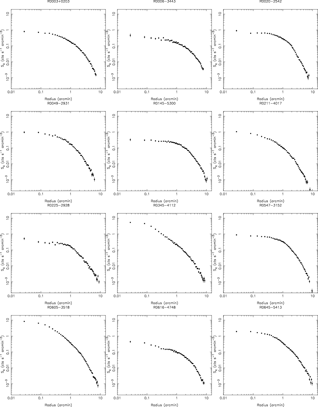 |
Figure A.1: Co-added MOS1, MOS2 and pn surface brightness profiles for the entire sample in the energy band 0.3-2.0 keV. |
| Open with DEXTER | |
In the text
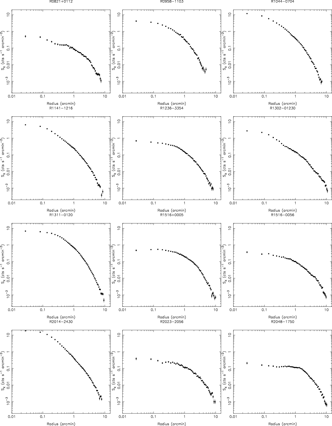 |
Figure A.1: continued. |
| Open with DEXTER | |
In the text
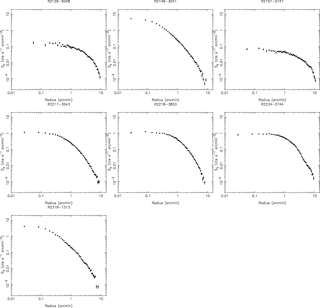 |
Figure A.1: continued. |
| Open with DEXTER | |
In the text
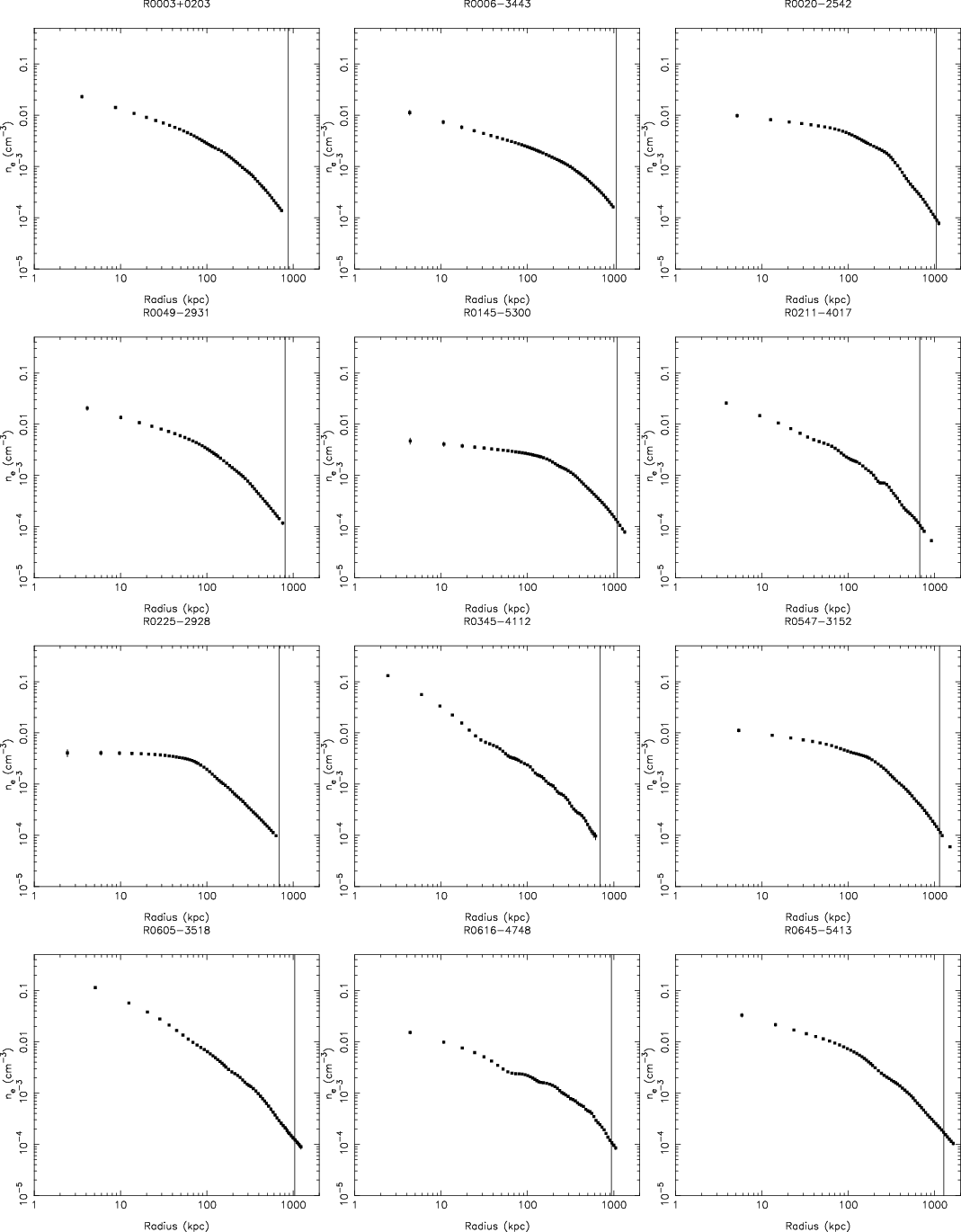 |
Figure A.2: Individual gas density profiles for the entire sample. Vertical lines indicate R500 for each cluster. |
| Open with DEXTER | |
In the text
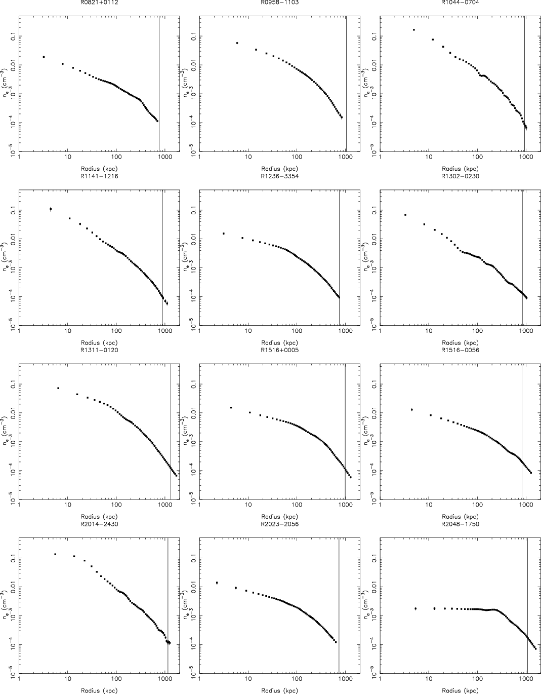 |
Figure A.2: continued. |
| Open with DEXTER | |
In the text
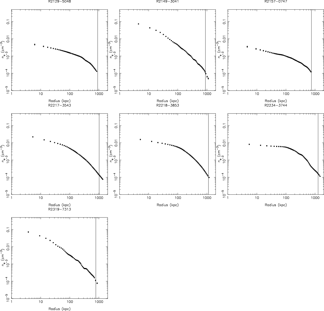 |
Figure A.2: continued. |
| Open with DEXTER | |
In the text