 |
(1) |
A&A 486, 819-828 (2008)
DOI: 10.1051/0004-6361:20078683
H. Men1,2 - K. Ferrière2 - J. L. Han1
1 - National Astronomical Observatories, Chinese Academy of Sciences,
Jia 20 DaTun Road, Chaoyang District, Beijing 100012, PR China
2 - Observatoire Midi-Pyrénées, Université Paul Sabatier Toulouse 3,
CNRS, 14 Av. Ed. Belin, 31400 Toulouse, France
Received 17 September 2007 / Accepted 8 May 2008
Abstract
Aims. Our purpose is to place firm observational constraints on the three most widely used theoretical models for the spatial configuration of the large-scale interstellar magnetic field in the Galactic disk, namely, the ring, the axisymmetric, and the bisymmetric field models.
Methods. We used the rotation measures (RMs) of low-latitude Galactic pulsars and combined them with their dispersion measures and estimated distances to map out the line-of-sight component of the interstellar magnetic field in the near half of the Galactic disk. We then fit our map of the line-of-sight field to the three aforementioned theoretical field models and discuss the acceptability of each fit, in order to determine whether the considered field model is allowed by the pulsar data or not.
Results. Strictly speaking, we find that all three field models are ruled out by the pulsar data. Furthermore, none of them appears to perform significantly better than the others. From this we conclude that the large-scale interstellar magnetic field in the Galactic disk has a more complex pattern than just circular, axisymmetric, or bisymmetric.
Key words: ISM: magnetic fields - Galaxy: disk - galaxies: magnetic fields
The interstellar magnetic field of our Galaxy has been the object of
intense investigation since the early 1980s. Different observational
methods (e.g., based on synchrotron emission, Faraday rotation,
Zeeman splitting, polarization of starlight, polarization of
dust infrared emission) provide information on the magnetic field in
different interstellar regions. Faraday rotation of Galactic pulsars
and extragalactic linearly polarized radio sources make it possible
to directly trace the magnetic field in ionized regions. In
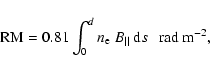
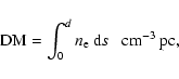
practice, one measures the so-called rotation measure (RM), defined
by
|
(1) |
 |
(2) |
We now know that the interstellar medium (ISM) is highly inhomogeneous
and that the interstellar magnetic field has an important turbulent
component. For this reason, neighboring pulsars may have significantly
different values of RM and DM, and a plot RM versus DM will
generally exhibit a large scatter.
However, if one considers a Galactic region larger than the scale of
the turbulent field and containing enough pulsars for statistical
purposes, one can infer the large-scale (or regular) component of
![]() in that region from the slope of the mean
DM-RM relation (Rand & Lyne 1994):
in that region from the slope of the mean
DM-RM relation (Rand & Lyne 1994):
In principle, RM studies are ideally suited to establish the overall structure of the Galactic magnetic field. However, the different RM studies performed so far yield contradictory results: some favor a ring field (Rand & Kulkarni 1989; Vallée 2005; Rand & Lyne 1994), others an axisymmetric or ASS field (Vallée 1996,1991), and others a bisymmetric or BSS field (Simard-Normandin & Kronberg 1980; Han & Qiao 1994; Indrani & Deshpande 1999; Han et al. 2006). Moreover, although all these studies conclude with a preferred field model, none of them has seriously considered the possibility that more than one model is allowed by the RM data or, alternatively, that none of the three basic models alone can account for the data. Hence the question we would like to address in this paper: which among the ring, axisymmetric and bisymmetric models can clearly be accepted on the grounds that it is consistent with the RM data, and which model should clearly be rejected on the grounds that it fails to provide a good fit to the data.
In recent years, numerous pulsars were discovered in the near half
of the Galactic disk and many of them had their RM measured.
At the present time, among the ![]() 1800 known pulsars,
690 have measured RMs and, among the latter, 524 are located at low
Galactic latitudes (
1800 known pulsars,
690 have measured RMs and, among the latter, 524 are located at low
Galactic latitudes (
![]() ). Pulsars with measured RMs now
provide a reasonably good coverage of the near half of the Galactic
disk. Furthermore, pulsar distances can now be estimated with fairly
good accuracy thanks to the improved free-electron density model of
Cordes & Lazio (2002) (known as the NE2001 model). The new measurements
enable one to investigate the configuration of the Galactic magnetic
field over a much larger region and with much more confidence than
previously feasible.
). Pulsars with measured RMs now
provide a reasonably good coverage of the near half of the Galactic
disk. Furthermore, pulsar distances can now be estimated with fairly
good accuracy thanks to the improved free-electron density model of
Cordes & Lazio (2002) (known as the NE2001 model). The new measurements
enable one to investigate the configuration of the Galactic magnetic
field over a much larger region and with much more confidence than
previously feasible.
In Sect. 2, we present the three basic theoretical models for the interstellar magnetic field in the Galactic disk. In Sect. 3, we describe the procedure used to bin the pulsar data and to map out the distribution of B||. In Sect. 4, we fit our map of B|| to each of the three field models, and we discuss how good the fits are at reproducing the pulsar data. In Sect. 5, we summarize our results and conclude our study.
Throughout this paper, the Galactocentric cylindrical coordinates
are denoted by
![]() ,
and the distance from the Galactic
center (GC) to the Sun is set to
,
and the distance from the Galactic
center (GC) to the Sun is set to
![]() .
.
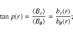
In general, the horizontal position of a given pulsar P can be defined either
by its distance from the GC, r, and its Galactic azimuthal angle ![]() (which increases clockwise from
(which increases clockwise from ![]() along the line
segment GC-Sun), or by its distance from the Sun, d, and its Galactic
longitude, l (which increases counterclockwise from l=0 along
the line segment Sun-GC). Another useful angular coordinate is the angle
along the line
segment GC-Sun), or by its distance from the Sun, d, and its Galactic
longitude, l (which increases counterclockwise from l=0 along
the line segment Sun-GC). Another useful angular coordinate is the angle ![]() between the azimuthal direction at P and the vector P-Sun,
such that
between the azimuthal direction at P and the vector P-Sun,
such that
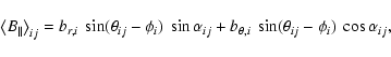
![]() (see Fig. 1).
(see Fig. 1).
![\begin{figure}
\par\includegraphics[angle=-90,width=6cm,clip]{8683fig1.ps}
\end{figure}](/articles/aa/full/2008/30/aa8683-07/img36.gif) |
Figure 1: Schematics showing the geometrical variables associated with a pulsar P (see main text for the exact definitions). |
| Open with DEXTER | |
Because Galactic differential rotation efficiently stretches magnetic field
lines in the azimuthal direction,
![]() dominates over
both
dominates over
both
![]() and
and
![]() .
Moreover, all the pulsars selected for the present work lie at
.
Moreover, all the pulsars selected for the present work lie at
![]() and reside in the Galactic disk.
There, the large-scale magnetic field is nearly horizontal
(e.g., Ruzmaikin et al. 1985; Beck et al. 1996), so that
and reside in the Galactic disk.
There, the large-scale magnetic field is nearly horizontal
(e.g., Ruzmaikin et al. 1985; Beck et al. 1996), so that
![]() .
In addition, projecting an already small
.
In addition, projecting an already small
![]() onto
the line of sight to a pulsar further reduces its contribution
by a factor
onto
the line of sight to a pulsar further reduces its contribution
by a factor
![]() .
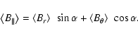
Under these conditions, the line-of-sight component of the large-scale
magnetic field depends only on its radial and azimuthal components,
and is related to them through
.
Under these conditions, the line-of-sight component of the large-scale
magnetic field depends only on its radial and azimuthal components,
and is related to them through
We now present the three theoretical field models.
In the ring model, the large-scale magnetic field points everywhere in
the azimuthal direction, so that its radial component vanishes:
![\begin{figure*}
\par\includegraphics[angle=-90,width=12.3cm,clip]{8683fig2a.ps}\...
...m}
\par\includegraphics[angle=-90,width=12.3cm,clip]{8683fig2b.ps}
\end{figure*}](/articles/aa/full/2008/30/aa8683-07/img49.gif) |
Figure 2:
Grids used in our study overlaid on the face-on distribution of our
482 low-latitude (
|
| Open with DEXTER | |
In the axisymmetric model,
![]() and
and
![]() are both independent of
are both independent of ![]() and vary only with r:
and vary only with r:
In the bisymmetric model,
![]() and
and
![]() have a simple sinusoidal dependence on
have a simple sinusoidal dependence on ![]() ,
which can be written
in the form
(Berkhuijsen et al. 1997):
,
which can be written
in the form
(Berkhuijsen et al. 1997):
To date, there are 690 pulsars with measured RMs (Hamilton & Lyne 1987; Qiao et al. 1995; van Ommen et al. 1997; Rand & Lyne 1994; Noutsos et al. 2008; Weisberg et al. 2004; Han et al. 1999; Mitra et al. 2003; Han et al. 2006; Crawford et al. 2001).
Among these pulsars, we selected those that lie at low Galactic
latitudes (
![]() )
and have reliable RMs
(error on
)
and have reliable RMs
(error on
![]() ).
This left us with 482 pulsars.
For the distances and DMs of our selected pulsars, we used the values
given in the ATNF Pulsar Catalog (Manchester et al. 2005,
see http://www.atnf.csiro.au/research/pulsar/psrcat).
Pulsar distances in this catalog were estimated with the help
of Cordes & Lazio's (2002) NE2001 model for the
free-electron density; for pulsars located in the inner Galaxy,
individual distances are typically uncertain by
).
This left us with 482 pulsars.
For the distances and DMs of our selected pulsars, we used the values
given in the ATNF Pulsar Catalog (Manchester et al. 2005,
see http://www.atnf.csiro.au/research/pulsar/psrcat).
Pulsar distances in this catalog were estimated with the help
of Cordes & Lazio's (2002) NE2001 model for the
free-electron density; for pulsars located in the inner Galaxy,
individual distances are typically uncertain by ![]()
![]() ,
but
the relative distances of neighboring pulsars have a much lower
uncertainty. Pulsar DMs, for their part, are known with good accuracy
(error on
,
but
the relative distances of neighboring pulsars have a much lower
uncertainty. Pulsar DMs, for their part, are known with good accuracy
(error on ![]() generally <
generally <
![]() ).
).
In order to map out the large-scale component of
![]() ,
one needs to divide the Galactic disk into
regions (boxes) having sizes intermediate between the large scales
of the regular field and the small scales of the turbulent field
and containing at least a few pulsars each. In previous studies
(Weisberg et al. 2004; Han et al. 2006; Rand & Lyne 1994), this division was based on a
heliocentric grid defined by circles of constant d and radial
lines of constant l. Such a heliocentric division was justified
by the spatial distribution of the available pulsars, but it is
ill-suited to the present work, whose purpose is to test field
models expressed in terms of Galactic radius, r. A much more
appropriate division here is one based on a hybrid grid defined by
circles of constant r and lines of constant l (see
Fig. 2).
To make full use of the pulsar data, we consider two different grids.
In the first grid, the circles are located at
,
one needs to divide the Galactic disk into
regions (boxes) having sizes intermediate between the large scales
of the regular field and the small scales of the turbulent field
and containing at least a few pulsars each. In previous studies
(Weisberg et al. 2004; Han et al. 2006; Rand & Lyne 1994), this division was based on a
heliocentric grid defined by circles of constant d and radial
lines of constant l. Such a heliocentric division was justified
by the spatial distribution of the available pulsars, but it is
ill-suited to the present work, whose purpose is to test field
models expressed in terms of Galactic radius, r. A much more
appropriate division here is one based on a hybrid grid defined by
circles of constant r and lines of constant l (see
Fig. 2).
To make full use of the pulsar data, we consider two different grids.
In the first grid, the circles are located at
![]() (i.e., r=ri, with
(i.e., r=ri, with
![]() ), and
the lines of constant l are the lines emanating from the Sun and
tangent to one of the circles
), and
the lines of constant l are the lines emanating from the Sun and
tangent to one of the circles
![]() ,
plus the line Sun-GC
(i.e.,
,
plus the line Sun-GC
(i.e.,
![]() ,
with
,
with
![]() and
and
![]() )
(see Fig. 2a).
The second grid is defined in an analogous manner with the circles shifted
by 0.5 kpc (i.e.,
)
(see Fig. 2a).
The second grid is defined in an analogous manner with the circles shifted
by 0.5 kpc (i.e.,
![]() ,
and accordingly,
,
and accordingly,
![]() )
(see Fig. 2b).
To ensure a sufficient number of pulsars per box, some of the boxes
defined by these grids are paired together.
More specifically, the non-outermost boxes along each ring are paired
either with their left or right neighbor along the same ring (thereby
leading to a single double-size box) or with both neighbors separately
(thereby leading to two overlapping boxes).
)
(see Fig. 2b).
To ensure a sufficient number of pulsars per box, some of the boxes
defined by these grids are paired together.
More specifically, the non-outermost boxes along each ring are paired
either with their left or right neighbor along the same ring (thereby
leading to a single double-size box) or with both neighbors separately
(thereby leading to two overlapping boxes).
Altogether, we have 9 rings, which are centered on
![]() ,
with
i= 4.5, 5.5 ... 7.5 in the first grid and
i= 4, 5 ... 8 in the second grid. In the following, the ring centered on ri (and
extending between ri-0.5 and ri+0.5) is referred to as ring i.
,
with
i= 4.5, 5.5 ... 7.5 in the first grid and
i= 4, 5 ... 8 in the second grid. In the following, the ring centered on ri (and
extending between ri-0.5 and ri+0.5) is referred to as ring i.
We retain only the boxes containing at least 5 RMs. This minimum number of RMs, which is smaller than generally recommended for statistical testing, results from the limited number of pulsars with know RMs; it was chosen as a trade-off between the need to have enough data points per box to make use of Eq. (4) and the need to have enough boxes on the Galactic plane to capture the spatial variations of the large-scale magnetic field. Even with such a small number of RMs in a given box, it is possible to trace the dependences of RM on distance and on DM for the pulsars lying in this box (see Weisberg et al. 2004; Han et al. 2006; Rand & Lyne 1994).
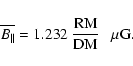
We estimate the average value of
![]() ,
denoted by
,
denoted by
![]() ,
in each of the retained boxes
in the following way: we plot the points (DM, RM) of all the pulsars
in the box, we fit a straight line through the resulting set of data points,
and we take
,
in each of the retained boxes
in the following way: we plot the points (DM, RM) of all the pulsars
in the box, we fit a straight line through the resulting set of data points,
and we take
![]() to be 1.232 times the slope
of this line (see Eq. (4) and preceding comment).
To perform the straight-line fit, we resort to a slightly modified
version of the ordinary least-squares linear regression of Y on X described by Isobe et al. (1990),
which is well suited when the dispersion of the data points about
the linear relation cannot be calculated beforehand.
The modifications brought to the original scheme are designed to exclude
the occasional outliers - such as those arising from H II regions
(Mitra et al. 2003). In practice, we discard all the data points
whose absolute deviation from the mean RM or DM exceeds three times
the mean absolute deviation.
To illustrate the procedure, we show two examples in Fig. 3.
to be 1.232 times the slope
of this line (see Eq. (4) and preceding comment).
To perform the straight-line fit, we resort to a slightly modified
version of the ordinary least-squares linear regression of Y on X described by Isobe et al. (1990),
which is well suited when the dispersion of the data points about
the linear relation cannot be calculated beforehand.
The modifications brought to the original scheme are designed to exclude
the occasional outliers - such as those arising from H II regions
(Mitra et al. 2003). In practice, we discard all the data points
whose absolute deviation from the mean RM or DM exceeds three times
the mean absolute deviation.
To illustrate the procedure, we show two examples in Fig. 3.
![\begin{figure}
\par\includegraphics[angle=-90,width=9cm,clip]{8683fig3a.ps}\bigskip\\
\includegraphics[angle=-90,width=9cm,clip]{8683fig3b.ps}
\end{figure}](/articles/aa/full/2008/30/aa8683-07/img71.gif) |
Figure 3:
Plots of RM versus distance ( left panels) and versus DM
( right panels) for the pulsars lying in two different boxes.
The first box ( top row) is delimited by the circles r=r5.5 and
r=r6.5 in the radial direction and by the tangential lines
l=l5.5 and l=l6.5 in the longitudinal direction.
The second box ( bottom row) is delimited by the circles r=r6.5 and
r=r7.5 and by the tangential lines l=l4.5 and l=l6.5.
For each box, the best-fit straight line through the points (DM, RM)
is drawn in the right panel, and the corresponding value of
|
| Open with DEXTER | |
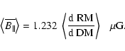
The derived values of
![]() in all the boxes of our two grids are mapped in Fig. 4.
For convenience, these values are converted into vectors oriented along
the local line of sight.
in all the boxes of our two grids are mapped in Fig. 4.
For convenience, these values are converted into vectors oriented along
the local line of sight.
As explained above Eq. (4), the turbulent component
of the magnetic field,
![]() ,
causes the RMs to scatter
about the mean DM-RM line. This physical scatter due to turbulence
is typically one order of magnitude larger than the observational
scatter due to measurement errors. The amplitude of the RM scatter
is given by the rms deviation of the measured RMs from the mean
DM-RM line. Since the RM scatter is of predominantly turbulent origin,
its amplitude divided by the mean DM in the considered box directly yields
(to a factor 1.232) an estimate for the rms value of the turbulent
component of the line-of-sight field,
,
causes the RMs to scatter
about the mean DM-RM line. This physical scatter due to turbulence
is typically one order of magnitude larger than the observational
scatter due to measurement errors. The amplitude of the RM scatter
is given by the rms deviation of the measured RMs from the mean
DM-RM line. Since the RM scatter is of predominantly turbulent origin,
its amplitude divided by the mean DM in the considered box directly yields
(to a factor 1.232) an estimate for the rms value of the turbulent
component of the line-of-sight field,
![]() .
Finally, the rms value of
.
Finally, the rms value of
![]() divided by
the square root of the number of pulsars in the box provides an estimate
for the statistical uncertainty in
divided by
the square root of the number of pulsars in the box provides an estimate
for the statistical uncertainty in
![]() ,
,
![]() ,
which, again, is predominantly due to turbulence.
The exact expression of
,
which, again, is predominantly due to turbulence.
The exact expression of
![]() can be found in Isobe et al. (1990).
With our data, the typical values of
can be found in Isobe et al. (1990).
With our data, the typical values of
![]() lie between
lie between
![]()
![]() and
and
![]() .
.
![\begin{figure}
\par\includegraphics[angle=-90,width=12cm]{8683fig4.ps}
\end{figure}](/articles/aa/full/2008/30/aa8683-07/img77.gif) |
Figure 4:
Face-on map showing the average line-of-sight component of the magnetic
field,
|
| Open with DEXTER | |
Once we have obtained a set of observational values of
![]() together with their statistical
uncertainties (or error bars), we can put the three theoretical
field models presented in Sect. 2 to the test.
As in all other studies based on RMs, we proceed on the notion that
the large-scale interstellar magnetic field may be identified with
its
together with their statistical
uncertainties (or error bars), we can put the three theoretical
field models presented in Sect. 2 to the test.
As in all other studies based on RMs, we proceed on the notion that
the large-scale interstellar magnetic field may be identified with
its ![]() -weighted average value (denoted with an overbar).
Implicit here is the assumption that fluctuations in magnetic field
strength and in free-electron density are statistically uncorrelated.
In reality, this assumption is certainly not strictly satisfied in the ISM
(e.g., Beck et al. 2003), and this will cause our results to be somewhat biased.
-weighted average value (denoted with an overbar).
Implicit here is the assumption that fluctuations in magnetic field
strength and in free-electron density are statistically uncorrelated.
In reality, this assumption is certainly not strictly satisfied in the ISM
(e.g., Beck et al. 2003), and this will cause our results to be somewhat biased.
With this caveat in mind, we now describe the overall procedure.
For each model, we use all our observational values
of
![]() to derive the best-fit
parameters of the model. We then examine whether the best fit is
consistent with the pulsar data, i.e., whether the theoretical
line-of-sight fields predicted by it fall within the error bars
of the observational
to derive the best-fit
parameters of the model. We then examine whether the best fit is
consistent with the pulsar data, i.e., whether the theoretical
line-of-sight fields predicted by it fall within the error bars
of the observational
![]() (in a statistical sense).
If we find that the best fit is not consistent with the data,
we may conclude that the considered model must be rejected.
If, on the other hand, the best fit is found consistent with the data,
we may conclude that the model is acceptable; we then determine
the extent of the so-called ``consistency domain'', i.e.,
the parameter domain around the best fit within which solutions
are consistent with the data.
(in a statistical sense).
If we find that the best fit is not consistent with the data,
we may conclude that the considered model must be rejected.
If, on the other hand, the best fit is found consistent with the data,
we may conclude that the model is acceptable; we then determine
the extent of the so-called ``consistency domain'', i.e.,
the parameter domain around the best fit within which solutions
are consistent with the data.
It is important to realize that the concept of acceptability differs from the concept of detectability. A given field model, say, the ring model, is acceptable only if it is not ruled out by the available pulsar data. This does not necessarily imply that the Galactic magnetic field is really of the ring type, nor that a ring field has truly been detected. Detection of a ring field requires not only that the ring model be acceptable, but also that the zero-field solution do not belong to the consistency domain.
Let us now discuss more specifically what exact criterion should be
used to test consistency with the pulsar data for a given field model.
Each of the three models is characterized by a number of independent
free functions of Galactic radius
(
![]() in the ring model;
in the ring model;
![]() and
and
![]() in the axisymmetric model; br(r),
in the axisymmetric model; br(r),
![]() and
and ![]() in the bisymmetric model), corresponding to the same number of
independent free parameters in every ring i
(denoted by
in the bisymmetric model), corresponding to the same number of
independent free parameters in every ring i
(denoted by
![]() in the ring model;
in the ring model;
![]() and
and
![]() in the axisymmetric model;
br,i,
in the axisymmetric model;
br,i,
![]() and
and ![]() in the bisymmetric model).
Therefore, the 9 different rings may be analyzed separately.
in the bisymmetric model).
Therefore, the 9 different rings may be analyzed separately.
For any one of the three field models, consider a given ring i
and suppose that this ring contains ni boxes.
For every box j, we have derived an observational value of
the average line-of-sight field
![]() ,
denoted by
,
denoted by
![]() ,
together with
its statistical uncertainty, denoted by
,
together with
its statistical uncertainty, denoted by
![]() .
Besides, we can calculate a theoretical expression of the large-scale
line-of-sight field
.
Besides, we can calculate a theoretical expression of the large-scale
line-of-sight field
![]() ,
denoted by
,
denoted by
![]() ,
in terms of the free parameters of ring i.
The best-fit values of these parameters are obtained by minimizing
,
in terms of the free parameters of ring i.
The best-fit values of these parameters are obtained by minimizing
The best fit of ring i can be considered consistent with the pulsar data
if, on average over ring i, the theoretical best-fit
![]() do not differ from the observational
do not differ from the observational
![]() by more than the associated uncertainties
by more than the associated uncertainties
![]() .
In mathematical terms, this condition for consistency can be expressed as
.
In mathematical terms, this condition for consistency can be expressed as
![]() .
However, when the number of data points, ni, is not much greater than
the number of free parameters,
.
However, when the number of data points, ni, is not much greater than
the number of free parameters, ![]() (
(![]() for the ring model;
for the ring model;
![]() for the axisymmetric model;
for the axisymmetric model; ![]() for the bisymmetric model),
consistency with the data should be tested with the more exact criterion
for the bisymmetric model),
consistency with the data should be tested with the more exact criterion
It is possible to obtain a more rigorous (and, at the same time,
more flexible) criterion for consistency.
Suppose, for the sake of argument, that the model we are testing is correct.
If the data points
![]() of ring i
follow a Gaussian distribution,
of ring i
follow a Gaussian distribution, ![]() has a chi-square distribution
with
has a chi-square distribution
with ![]() degrees of freedom.
One can then calculate the a priori probability,
degrees of freedom.
One can then calculate the a priori probability,
![]() ,
that the
,
that the ![]() obtained
for a particular set of data points exceeds some critical value
obtained
for a particular set of data points exceeds some critical value
![]() .
Conversely, one can calculate the critical
.
Conversely, one can calculate the critical
![]() for which
for which
![]() equals some imposed
probability P0.
For instance, if the model is correct, it is unlikely (only 10% chance)
that
equals some imposed
probability P0.
For instance, if the model is correct, it is unlikely (only 10% chance)
that
![]() .
Turning the statement around,
if we find
.
Turning the statement around,
if we find
![]() ,
it is unlikely that
the model is correct - we will say that the model is inconsistent
with the data.
This reasoning directly leads to the following consistency condition:
,
it is unlikely that
the model is correct - we will say that the model is inconsistent
with the data.
This reasoning directly leads to the following consistency condition:
In the next three subsections, we present the results obtained with the rule of thumb (Eq. (14)) and with the more rigorous consistency condition (Eq. (15)), for the three field models.
In the ring model,
![]() vanishes and
vanishes and
![]() is constant along circles. Hence, there are 9 free parameters:
is constant along circles. Hence, there are 9 free parameters:
![]() ,
the large-scale azimuthal fields
in the 9 rings
i= 4, 4.5, 5 ... 8
,
the large-scale azimuthal fields
in the 9 rings
i= 4, 4.5, 5 ... 8![]() .
Since all the free parameters are independent, the 9 rings can be treated
separately.
.
Since all the free parameters are independent, the 9 rings can be treated
separately.
For every ring i, the large-scale line-of-sight field in any box j
is simply the projection of
![]() onto the line of
sight (see Eq. (5) with
onto the line of
sight (see Eq. (5) with
![]() ):
):
The values of
![]() and their uncertainties
and their uncertainties
![]() in the ni boxes jof the 9 rings i are plotted in Fig. 5,
at the Galactic azimuthal angles of the box midpoints,
in the ni boxes jof the 9 rings i are plotted in Fig. 5,
at the Galactic azimuthal angles of the box midpoints,
![]() .
For comparison, the best-fit values of
.
For comparison, the best-fit values of
![]() in the 9 rings are indicated by horizontal lines spanning the entire
azimuthal range.
in the 9 rings are indicated by horizontal lines spanning the entire
azimuthal range.
![\begin{figure}
\par\includegraphics[angle=-90,width=9cm,clip]{8683fig5.ps}
\end{figure}](/articles/aa/full/2008/30/aa8683-07/img112.gif) |
Figure 5:
Observational values of the average azimuthal fields,
|
| Open with DEXTER | |
Table 1:
Critical values of ![]() for 3 probability levels.
for 3 probability levels.
In only one ring (i=4.5) does the best-fit value of
![]() satisfy the rule-of-thumb
consistency condition,
satisfy the rule-of-thumb
consistency condition,
![]() (Eq. (14) with
(Eq. (14) with ![]() ).
For this ring, we compute the consistency range of
).
For this ring, we compute the consistency range of
![]() ,
which contains all the values of
,
which contains all the values of
![]() for which
for which
![]() .
The best-fit value of
.
The best-fit value of
![]() and its consistency
range in the sole ``good-fit'' ring are plotted against ri,
in the upper panel of Fig. 6.
For the other 8 rings, the (inconsistent) best-fit values of
and its consistency
range in the sole ``good-fit'' ring are plotted against ri,
in the upper panel of Fig. 6.
For the other 8 rings, the (inconsistent) best-fit values of
![]() are plotted with crosses.
Clearly, these 8 rings do not admit any ring magnetic field
consistent with the data.
As an immediate consequence, the ring model must be rejected.
are plotted with crosses.
Clearly, these 8 rings do not admit any ring magnetic field
consistent with the data.
As an immediate consequence, the ring model must be rejected.
In order to gain some feel for how far the ring model is from being
able to reproduce the pulsar data, let us, in thought, extend the
error bars of all the observational
![]() by a factor of 2 and look into
the impact of this extension on our results. With twice the original
error bars, the
by a factor of 2 and look into
the impact of this extension on our results. With twice the original
error bars, the ![]() parameter would be smaller by a factor of 4,
so that, in terms of the original
parameter would be smaller by a factor of 4,
so that, in terms of the original ![]() ,
the rule-of-thumb
consistency condition would become
,
the rule-of-thumb
consistency condition would become
![]() .
As it turns out, this less stringent consistency condition would be
fulfilled in 5 rings (
i=4, 4.5, 5.5, 6, 7)
out of 9. Thus, with twice the original error bars, the ring model
would remain unacceptable.
.
As it turns out, this less stringent consistency condition would be
fulfilled in 5 rings (
i=4, 4.5, 5.5, 6, 7)
out of 9. Thus, with twice the original error bars, the ring model
would remain unacceptable.
If we now resort to the more rigorous consistency condition,
![]() (Eq. (15) with P0=0.1),
to test the ring model, we find that 3 rings (
i=4, 4.5, 6)
have their best-fit
(Eq. (15) with P0=0.1),
to test the ring model, we find that 3 rings (
i=4, 4.5, 6)
have their best-fit
![]() consistent with the data;
their consistency ranges are drawn in the lower panel of
Fig. 6.
For the other 6 rings, the (inconsistent) best-fit
consistent with the data;
their consistency ranges are drawn in the lower panel of
Fig. 6.
For the other 6 rings, the (inconsistent) best-fit
![]() are again plotted with crosses.
With P0=0.05, 4 rings (
i=4, 4.5, 6, 7) would be deemed
consistent with the data, but the other 5 rings would still fail
the consistency test.
are again plotted with crosses.
With P0=0.05, 4 rings (
i=4, 4.5, 6, 7) would be deemed
consistent with the data, but the other 5 rings would still fail
the consistency test.
These results confirm our conclusion that the ring model must be rejected.
In the axisymmetric model,
![]() and
and
![]() are both constant along circles. Hence, there are 18 free parameters:
are both constant along circles. Hence, there are 18 free parameters:
![]() and
and
![]() ,
the large-scale radial and azimuthal fields
in the 9 rings
i= 4, 4.5, 5 ... 8.
,
the large-scale radial and azimuthal fields
in the 9 rings
i= 4, 4.5, 5 ... 8.
For every ring i, the large-scale line-of-sight field in any box j
can be written as a linear combination of the two parameters
![]() and
and
![]() :
:
![\begin{figure}
\par\includegraphics[angle=-90,width=8cm,clip]{8683fig6.ps}
\end{figure}](/articles/aa/full/2008/30/aa8683-07/img118.gif) |
Figure 6:
Best-fit values of the model parameters,
|
| Open with DEXTER | |
Here, we find that 1 ring (i= 4.5) has its best fit
consistent with the data, according to the rule-of-thumb consistency
condition,
![]() (Eq. (14) with
(Eq. (14) with ![]() ).
Its consistency domain in the parameter plane
).
Its consistency domain in the parameter plane
![]() is the area delimited by the ellipse
is the area delimited by the ellipse
![]() (grey contour line in the relevant panel of Fig. 7).
As none of the other 8 rings can be properly fit with an axisymmetric
magnetic field, the axisymmetric model must be rejected.
(grey contour line in the relevant panel of Fig. 7).
As none of the other 8 rings can be properly fit with an axisymmetric
magnetic field, the axisymmetric model must be rejected.
With twice the original error bars on the observational
![]() ,
the rule-of-thumb consistency
condition would become
,
the rule-of-thumb consistency
condition would become
![]() (in terms of the
original
(in terms of the
original ![]() ).
This less stringent consistency condition would be satisfied in 5 rings
(
i=4, 4.5, 6, 7, 8), but still not in the other 4 rings.
Therefore, the axisymmetric model would remain unacceptable.
).
This less stringent consistency condition would be satisfied in 5 rings
(
i=4, 4.5, 6, 7, 8), but still not in the other 4 rings.
Therefore, the axisymmetric model would remain unacceptable.
According to the more rigorous consistency condition,
![]() (Eq. (15)
with P0=0.1), 5 rings (
i=4, 4.5, 6, 7, 8) have their best fits
consistent with the data.
Their consistency domains in the parameter planes
(Eq. (15)
with P0=0.1), 5 rings (
i=4, 4.5, 6, 7, 8) have their best fits
consistent with the data.
Their consistency domains in the parameter planes
![]() are the elliptical
areas enclosed by the curves
are the elliptical
areas enclosed by the curves
![]() (black contour lines in the relevant panels of Fig. 7).
For the other 4 rings, the (inconsistent) best-fit pairs
(black contour lines in the relevant panels of Fig. 7).
For the other 4 rings, the (inconsistent) best-fit pairs
![]() are indicated with crosses.
Relaxing the probability level to P0=0.05 would not raise
the number of acceptable rings above 5.
are indicated with crosses.
Relaxing the probability level to P0=0.05 would not raise
the number of acceptable rings above 5.
From all the above, we conclude that the axisymmetric model must be rejected.
In the bisymmetric model,
![]() and
and
![]() vary sinusoidally along circles in the manner described by
Eqs. (10) and (11).
Hence, there are 27 free parameters:
br,i,
vary sinusoidally along circles in the manner described by
Eqs. (10) and (11).
Hence, there are 27 free parameters:
br,i,
![]() and
and ![]() ,
the maximum amplitudes and
the azimuthal phases in the 9 rings
i= 4, 4.5, 5 ... 8.
,
the maximum amplitudes and
the azimuthal phases in the 9 rings
i= 4, 4.5, 5 ... 8.
For every ring i, the large-scale line-of-sight field in any box j
follows from Eq. (5) together with
Eqs. (10), (11):
![\begin{figure}
\par\includegraphics[angle=-90,width=12cm,clip]{8683fig7.ps}
\end{figure}](/articles/aa/full/2008/30/aa8683-07/img123.gif) |
Figure 7:
Consistency domains in the parameter planes
|
| Open with DEXTER | |
![\begin{figure}
\par\includegraphics[angle=-90,width=12cm,clip]{8683fig8.ps}
\end{figure}](/articles/aa/full/2008/30/aa8683-07/img124.gif) |
Figure 8:
Projections of the 3D consistency domains of the 9 different rings
on their parameter planes
|
| Open with DEXTER | |
According to the rule-of-thumb consistency condition,
![]() (Eq. (14) with
(Eq. (14) with ![]() ),
2 rings (i=4.5, 5) have their best fits consistent with the data.
Their consistency domains in the parameter spaces
),
2 rings (i=4.5, 5) have their best fits consistent with the data.
Their consistency domains in the parameter spaces
![]() are the volumes bounded
by the surfaces
are the volumes bounded
by the surfaces
![]() .
Displayed in Fig. 8 are the projections of these
consistency domains on the parameter planes
.
Displayed in Fig. 8 are the projections of these
consistency domains on the parameter planes
![]() (grey contour lines).
Since the other 7 rings fail the consistency test, the bisymmetric model
must be rejected.
(grey contour lines).
Since the other 7 rings fail the consistency test, the bisymmetric model
must be rejected.
With twice the original error bars on the observational
![]() ,
the rule-of-thumb consistency
condition would become
,
the rule-of-thumb consistency
condition would become
![]() ,
which would be satisfied
in 7 rings (
i=4, 4.5, 5, 5.5, 6, 7, 8) out of 9.
The bisymmetric model would then be nearly acceptable.
,
which would be satisfied
in 7 rings (
i=4, 4.5, 5, 5.5, 6, 7, 8) out of 9.
The bisymmetric model would then be nearly acceptable.
According to the more rigorous consistency condition,
![]() (Eq. (15)
with P0=0.1), 5 rings (
i=4.5, 5, 6, 7, 8) have their best fits
consistent with the data.
Their consistency domains, bounded by the surfaces
(Eq. (15)
with P0=0.1), 5 rings (
i=4.5, 5, 6, 7, 8) have their best fits
consistent with the data.
Their consistency domains, bounded by the surfaces
![]() ,
are also shown in projection
on the parameter planes
,
are also shown in projection
on the parameter planes
![]() in Fig. 8
(black contour lines).
For the other 4 rings, the (inconsistent) best-fit pairs
in Fig. 8
(black contour lines).
For the other 4 rings, the (inconsistent) best-fit pairs
![]() are indicated with crosses.
Relaxing the probability level to P0=0.05 would raise the number
of acceptable rings to 7 (
i=4, 4.5, 5, 5.5, 6, 7, 8),
which would render the bisymmetric model nearly globally acceptable.
are indicated with crosses.
Relaxing the probability level to P0=0.05 would raise the number
of acceptable rings to 7 (
i=4, 4.5, 5, 5.5, 6, 7, 8),
which would render the bisymmetric model nearly globally acceptable.
Altogether, the bisymmetric model must be rejected, though its rejection is slightly less severe than for the axisymmetric model.
In this paper, we examined the three most common theoretical models for
the large-scale magnetic field in the Galactic disk and confronted each
of these models with the pulsar data.
For each model, we derived the best-fit parameters, through ![]() minimization, in the 9 Galactocentric rings defined in Fig. 2,
and we delineated the parameter domains around the best fits (referred to
as the consistency domains) wherein the predicted fields are consistent
with the pulsar data.
minimization, in the 9 Galactocentric rings defined in Fig. 2,
and we delineated the parameter domains around the best fits (referred to
as the consistency domains) wherein the predicted fields are consistent
with the pulsar data.
Compared to existing studies of the kind, we did not attempt to settle the long-standing (and possibly ill-posed) question of whether the Galactic magnetic field is axisymmetric or bisymmetric. Our sole purpose was to determine whether each of the three basic field models, taken separately, is compatible with the available pulsar data or not. In this regard, we note that many previous studies did find a preference for one of the field models, but omitted to put their preferred model through the crucial ``goodness-of-fit'' test, which checks whether the model can indeed reproduce the data within the error bars.
Here, we tested the three field models on the basis of two different
criteria: first, a standard rule of thumb for a reasonably good fit
(Eq. (14)), and second, a more rigorous consistency
condition for a chi-square distribution of ![]() (Eq. (15), with the imposed probability
set to P0=0.1).
These two criteria were successively applied to all the rings separately,
such that the best fit of ring i was deemed consistent with the pulsar data
if the associated value of
(Eq. (15), with the imposed probability
set to P0=0.1).
These two criteria were successively applied to all the rings separately,
such that the best fit of ring i was deemed consistent with the pulsar data
if the associated value of ![]() ,
,
![]() ,
was less than
,
was less than ![]() (first criterion) or less than
(first criterion) or less than
![]() (second criterion).
A model could then be considered globally acceptable if all the rings
had their best fits consistent with the data.
(second criterion).
A model could then be considered globally acceptable if all the rings
had their best fits consistent with the data.
The results obtained for the three field models, with both criteria,
are summarized in Table 2.
All the rings are listed with their labels, i
(see footnote 1), and their numbers of boxes
(or numbers of data points), ni, from which it is straightforward
to deduce the numbers of degrees of freedom, ![]() (for the first
criterion), and the critical
(for the first
criterion), and the critical
![]() (for the second criterion; see Table 1).
Also given for all the rings are the minimum values of
(for the second criterion; see Table 1).
Also given for all the rings are the minimum values of ![]() ,
,
![]() ,
i.e., the values associated with the best fits,
as well as the results of both consistency tests (satisfaction of a test
is indicated with an asterisk), for the three field models.
,
i.e., the values associated with the best fits,
as well as the results of both consistency tests (satisfaction of a test
is indicated with an asterisk), for the three field models.
Table 2: Summary of the results obtained for the three field modelsa.
We found that none of the three field models is acceptable, in the sense that none of them can be brought into full agreement with the pulsar data. According to the standard rule-of-thumb consistency condition (Eq. (14)), all three models must be strongly rejected, as the ring and axisymmetric models fail to provide a good fit (consistent with the data) in all the rings save one, while the bisymmetric model fails in all the rings save two. If the error bars of the observational line-of-sight fields were enlarged by a factor of 2, the bisymmetric model would not be too far from acceptable (7 good-fit rings out of 9), while the ring and axisymmetric models would remain truly unacceptable (5 good-fit rings out of 9). The conclusions reached with the more rigorous consistency condition (Eq. (15)) are intermediate between the two situations described above: with the imposed probability set to P0=0.1 (P0=0.05), 3 (4) rings can be properly fit with a ring magnetic field, 5 (5) with an axisymmetric field and 5 (7) with a bisymmetric field.
The quantitative differences between both criteria are easily understood.
A comparison between Eqs. (14) and (15) immediately shows that the rule-of-thumb
consistency condition (Eq. (14)) corresponds to
a probability level P1 such that
![]() ,
or equivalently,
,
or equivalently,
![]() .
With twice the original error bars on the observational line-of-sight
fields, the rule-of-thumb consistency condition would become
.
With twice the original error bars on the observational line-of-sight
fields, the rule-of-thumb consistency condition would become
![]() ,
corresponding to a probability level P2
such that
,
corresponding to a probability level P2
such that
![]() ,
or equivalently,
,
or equivalently,
![]() .
The values of P1 and P2 as functions of
.
The values of P1 and P2 as functions of ![]() are tabulated in Table 3.
Clearly, the rule-of-thumb consistency condition with the original
error bars implies high probability levels (
are tabulated in Table 3.
Clearly, the rule-of-thumb consistency condition with the original
error bars implies high probability levels (
![]() ),
which make it overly difficult to satisfy; if the model under testing
is correct, there is nonetheless a
),
which make it overly difficult to satisfy; if the model under testing
is correct, there is nonetheless a ![]()
![]() chance
that
chance
that ![]() exceeds
exceeds ![]() and that the model will be rejected.
On the other hand, with twice the original error bars, the probability
levels drop very low (
and that the model will be rejected.
On the other hand, with twice the original error bars, the probability
levels drop very low (
![]() )
and the consistency condition
becomes too easily satisfied; the risk is then to accept a model that
is in fact incorrect.
)
and the consistency condition
becomes too easily satisfied; the risk is then to accept a model that
is in fact incorrect.
The bottom line is that the standard rule of thumb is way too stringent, while the rule of thumb with twice the original error bars is way too easy. In contrast, the more rigorous criterion with a probability level set to P0=0.1, intermediate between P1 and P2, provides a reasonable trade-off. The latter criterion is also more trustworthy, insofar as all the rings for all the models are tested with the same probability level.
The results of the present study suggest that the true large-scale magnetic field in our Galaxy has a more complex configuration than a strictly axisymmetric or bisymmetric field. One possibility is that it consists of the superposition of axisymmetric, bisymmetric and probably higher-order azimuthal modes. Such combinations of modes have been observed in a number of external galaxies (e.g., Beck 2007; Beck et al. 1996; Berkhuijsen et al. 1997; Rohde et al. 1999).
Table 3: Probability levels for the rule-of-thumb consistency condition.
Acknowledgements
We thank the referee for his/her valuable comments as well as Pierre Jean and William Gillard for useful discussions. J.L.H. and M.H. were supported by the National Natural Science Foundation (NNSF) of China (10521001 and 10773016) and the National Key Basic Research Science Foundation of China (2007CB815403). M.H. was also supported by the French Embassy in Beijing during her stay in Toulouse in the framework of a bilateral co-supervised Ph.D. program.