A&A 486, 951-970 (2008)
DOI: 10.1051/0004-6361:200809724
A grid of MARCS model atmospheres for late-type stars
I. Methods and general properties
B. Gustafsson1 - B. Edvardsson1 - K. Eriksson1 - U. G. Jørgensen2 - Å. Nordlund2 - B. Plez3,1
1 - Department of Physics and Astronomy, Uppsala Astronomical
Observatory, Box 515, 751 20 Uppsala, Sweden
2 - Niels Bohr Institute for Astronomy, Physics and Geophysics,
Copenhagen University, Blegdamsveg 17, Copenhagen Ø, 2100, Denmark
3 - GRAAL, Université de Montpellier II, 34095 Montpellier Cedex 05, France
Received 5 March 2008 / Accepted 30 April 2008
Abstract
Context. In analyses of stellar spectra and colours, and for the analysis of integrated light from galaxies, a homogeneous grid of model atmospheres of late-type stars and corresponding flux spectra is needed.
Aims. We construct an extensive grid of spherically-symmetric models (supplemented with plane-parallel ones for the highest surface gravities), built on up-to-date atomic and molecular data, and make it available for public use.
Methods. The most recent version of the MARCS program is used.
Results. We present a grid of about 104 model atmospheres for stars with


 ,
,
 log g = log
 (cgs) with various masses and radii,
![$-5 \le \rm [Me/H]\le +1$](/articles/aa/full/2008/30/aa09724-08/img47.gif) ,
with
,
with  Fe] = 0.0 and 0.4 and different choices of C and N abundances. This includes ``CN-cycled'' models with C/N = 4.07 (solar), 1.5 and 0.5, C/O ranging from 0.09 to (normally) 5.0 to also represent stars of spectral types R, S and N, and with
 km s-1. We also list thermodynamic quantities (T,
  ,
,
 ,
,
 ,
partial pressures of molecules, etc.) and provide them on the World Wide Web, as well as calculated fluxes in approximately 108 000 wavelength points. Underlying assumptions in addition to 1D stratification (spherical or plane-parallel) include hydrostatic equilibrium, mixing-length convection and local thermodynamic equilibrium. We discuss a number of general properties of the models, in particular in relation to the effects of changing abundances, of blanketing, and of sphericity. We illustrate positive and negative feedbacks between sphericity and molecular blanketing. We compare the models with those of other available grids and find excellent agreement with plane-parallel models of Castelli & Kurucz (if convection is treated consistently) within the overlapping parameter range. Although there are considerable departures from the spherically-symmetric NextGen models, the agreement with more recent PHOENIX models is gratifying.
,
partial pressures of molecules, etc.) and provide them on the World Wide Web, as well as calculated fluxes in approximately 108 000 wavelength points. Underlying assumptions in addition to 1D stratification (spherical or plane-parallel) include hydrostatic equilibrium, mixing-length convection and local thermodynamic equilibrium. We discuss a number of general properties of the models, in particular in relation to the effects of changing abundances, of blanketing, and of sphericity. We illustrate positive and negative feedbacks between sphericity and molecular blanketing. We compare the models with those of other available grids and find excellent agreement with plane-parallel models of Castelli & Kurucz (if convection is treated consistently) within the overlapping parameter range. Although there are considerable departures from the spherically-symmetric NextGen models, the agreement with more recent PHOENIX models is gratifying.
Conclusions. The models of the grid show considerable regularities, but some interesting departures from general patterns occur for the coolest models due to the molecular opacities. We have tested a number of approximate ``rules of thumb'' concerning effects of blanketing and sphericity and often found them to be astonishingly accurate. Some interesting new phenomena have been discovered and explored, such as the intricate coupling between blanketing and sphericity, and the strong effects of carbon enhancement on metal-poor models. We give further details of line absorption data for molecules, as well as details of models and comparisons with observations in subsequent papers.
Key words: stars: atmospheres - Sun: abundances - stars: fundamental parameters
- stars: general - stars: late-type - stars: supergiants
Since the first grids of line-blanketed, model atmospheres for late-type
stars were published (Carbon & Gingerich 1969;
Querci et al. 1974;
Peytremann 1974; Gustafsson et al. 1975;
Kurucz 1979; Johnson et al. 1980), there has been a very impressive
improvement in underlying data, in particular, for atomic and molecular
absorption. Accurate continuous absorption coefficients for a number
of heavy elements have been calculated within the Opacity Project
(Seaton et al. 1994), and the Iron Project (Bautista 1997).
The Opacity Project also contributed accurate transition probabilities
for a wealth of spectral lines for elements where the LS coupling
approximation was applicable. Thanks to systematic efforts by Kurucz
(see http://kurucz.harvard.edu) line lists with transition probabilities for
millions of lines of heavy elements have been calculated. Also, the
admirable and systematic work by experimental physicists (e.g. Blackwell et al. 1989; Nave et al. 1994;
Hartman et al. 2003; Lawler et al. 2007) has led to the identification and measurements
of many more metal transitions, e.g., from Fe I and Fe II,
than existed before.
The results of these efforts have been made easily accessible in data bases,
such as the Vienna Atomic Line Database, VALD (see Piskunov et al. 1995; Stempels et al. 2001;
see also http://www.astro.uu.se/~vald). Additional significant progress has been made in the calculation
of accurate damping constants for strong atomic lines (Anstee & O'Mara 1995; Barklem et al. 2000a) as well as for hydrogen self broadening (Barklem et al. 2000b).
Impressive progress has also been made in the study of molecular absorption
starting from practically nothing 30 years ago
(see Jørgensen 1994b, 2005, for
reviews). Very extensive line lists have thus been calculated for most diatomic
and polyatomic molecules that contribute opacity in stellar atmospheres.
The lists are based on laboratory measurements of wavelengths and gf values
with simple theoretical extensions, or are the result of more extensive
quantum-mechanical ab-initio calculations. Even if the absorption
cross-sections are not always of satisfactory quality as yet, the existence
of these lists makes it possible to calculate models for, e.g., M and C stars
that are realistic enough to compare reasonably well with observations.
Simultaneous with these improvements of basic physics, steps to improve
the physical consistency of the models have also been taken. The traditional
assumptions of plane-parallel stratification in homogenous layers, of
stationary hydrostatic equilibrium, mixing-length convection and local thermodynamic
equilibrium (LTE) have
stepwise been possible to relax. Grids of spherically-symmetric models
for giants and supergiants were made by Plez et al. (1992) and
Jørgensen et al. (1992). Dynamic pulsating model atmospheres for
cool giants have been developed by Wood (1979) and Bowen (1988), and these were
improved with time-dependent dust formation by Fleischer et al. (1992) and
Höfner & Dorfi (1997), and further developed to include frequency-dependent
radiative transfer by Höfner (1999) and
Höfner et al. (2003).
Nordlund & Stein and collaborators (Nordlund 1982;
Nordlund & Dravins 1990; Stein & Nordlund 1998;
Asplund et al. 1999, 2000a)
developed 3D simulations with proper hydrodynamics and radiation fields
taken into account for solar-type stars, and
Freytag (2001) developed full ``star-in-a-box'' models for supergiants.
These simulations show a striking agreement with observations
of solar granulation and spectral line profiles for solar type stars, and
clearly demonstrate the qualitative difference between traditional 1D models
and reality: while the temperature structure in the upper layers of the
1D models is determined by radiative cooling and heating, the radiative heating
in real late-type stars is balanced to a significant extent also by expansion
cooling of upwelling gas.
A consistent treatment of radiative transfer in models for late-type stars
without making the assumption of LTE is complicated due to the great number of
atomic and molecular species affecting the radiative field; the wealth of
levels and transitions in these species; and the lack of basic data for these
transitions - not the least of which is the lack of cross sections for atomic and molecular
collisions with electrons and hydrogen atoms. From the first attempt to
construct a reasonably realistic non-LTE model for a late-type star (the Sun) made
by Anderson (1989), the development of algorithms and computers has now made
it possible to calculate grids of such models (Hauschildt et al. 2002).
The lack
of accurate collision cross sections, however, is still a major problem in these
efforts.
In the present paper we present an extensive grid of model atmospheres for late-type
stars. The models are still classical, in the sense that they are one-dimensional, i.e., spherically
symmetric or plane-parallel, with LTE assumed and convection taken into account by using the
standard mixing-length theory. In spite of the inadequacy of these underlying physical
assumptions, which must be abandoned for detailed analysis of late-type
stellar spectra at high accuracy, we still think the present grid will be useful for years to come
for various applications extending from studies of individual stars to galactic
evolution and populations in external galaxies.
The grid extends from models for A-type stars to M, S, and
C star models, from dwarfs to supergiants in luminosity, from
10-5 times solar to 10 times solar in metallicity, and with various choices
of parameters like radius and mass, abundances of C, N, and O, of
`` elements'' (Ne, Mg, Si, S, Ar, Ca, Ti) relative to Fe, and of
microturbulence.
We also provide model spectral energy distributions (SEDs) sampled in about
105 frequency
points. With respect to methods and underlying data used, the model grid is
homogeneous.
elements'' (Ne, Mg, Si, S, Ar, Ca, Ti) relative to Fe, and of
microturbulence.
We also provide model spectral energy distributions (SEDs) sampled in about
105 frequency
points. With respect to methods and underlying data used, the model grid is
homogeneous.
The grid is presented in
a number of papers. In this initial paper, we (Sect. 2) sketch the development of our computer
code MARCS, from which models produced at different earlier stages are in wide use,
give a general outline of the methods now used (Sects. 3 and 4),
and underlying data (Sect. 5), as well as properties of the grid (Sect. 6). Models are also
compared with models from other contemporary grids (Sect. 7). In subsequent papers,
we shall discuss models for A-G stars (Edvardsson et al., Paper II),
K and R stars (Eriksson et al., Paper III), M stars (Plez et al., Paper IV),
S stars (Plez et al., Paper V), C stars (Jørgensen et al., Paper VI), and models for
very metal-poor stars (Paper VII). In
these subsequent papers, the most important new opacity data are described; the model
structures are described and analysed; and the model SEDs, fluxes and colours
are compared to some observational data to explore and illustrate the
applicability of the models. The total number of models is about 104. The details of these models,
including their calculated fluxes at different wavelengths,
are available via http://marcs.astro.uu.se.
Since the early 1970ies, we have developed and used the code MARCS
for constructing late-type model atmospheres. Spectral-line blanketing was
first considered using opacity distribution functions (ODFs, Gustafsson et al. 1975)
and this technique and its underlying ODF approximation was proven
to be fully adequate for F, G, and K stars. Thus, models could be calculated
with just a few hundred frequency points and extensive grids for G and K giants
(Bell et al. 1976) as well as R stars (Olander 1981) were issued on the basis of
the ODF approximation. The ODFs were
constructed with a program called SSG, originally devised for synthetic colour
calculations by Bell (see, e.g., Bell 1971). The line list used by this
program was based on laboratory wavelengths and oscillator strengths, as well as
``astrophysical oscillator strengths'' derived from the solar spectrum.
The total list contained about 50 000 lines. The SSG program was used next
to calculate model spectra and colours, which were systematically compared
with observations (e.g. Gustafsson & Bell 1979;
Bell & Gustafsson 1989).
From these comparisons, a generally good agreement was found, which gave us
the confidence to apply the models in a number of studies, e.g., of abundances
in globular cluster stars.
However, there was a mismatch in certain wavelength
regions, in particular in the ultraviolet and violet, where the models were
obviously too bright. We tentatively ascribed this discrepancy to the absence
in the line lists and the models of many weak lines, which together affect the
stellar spectra.
There were also more fundamental problems with the ODF method.
One was that the ODFs had to be recalculated when the chemical composition
was changed, which made it inflexible for stars with special and peculiar
abundances, such as carbon stars. To circumvent this, a special method to
add ODFs for individual molecules was invented (Saxner & Gustafsson 1984).
However, for N-type carbon star models, we also found that the effects
of molecules in the upper atmospheric layers, contributing strong opacity at
wavelengths different from the atomic absorption at greater depths, made the
ODF approximation unsatisfactory (cf., Ekberg et al. 1986). To provide satisfactory
analysis for a study of the chemical composition of carbon stars (Lambert
et al. 1986), we consequently changed the scheme to opacity sampling, in which
the adequate absorption at each monochromatic wavelength point is treated in
full detail (yet, assuming LTE in our case), following Peytremann (1974) and Sneden et al. (1976). In order to obtain an accurate
representation of the total radiation contribution to the heat balance and the
radiative pressure force, this required an increase of the number of frequency
points by one to two orders of magnitude. A number of model grids were calculated
with this new program, for carbon stars (cf., Lambert et al. 1986;
Jørgensen et al. 1992), for M giants
(Plez et al. 1992) and M dwarfs (Brett & Plez 1993) and
applied to studies of individual stars. We gradually extended the underlying
line list by calculating and adopting more complete data for diatomic molecules,
such as TiO (Jørgensen 1994a; Plez et al. 1992;
Plez 1998),
as well as polyatomic molecules like
HCN (Jørgensen et al. 1985; Jørgensen 1990),
C2H2 (Jørgensen thesis; cited
in Jørgensen 1989)
and H2O (Plez et al. 1992; Alvarez & Plez 1998;
Jørgensen et al. 2001; Decin et al. 2000).
In order to provide models for a major effort to study the build-up of chemical
elements in the Galactic disk using solar-type stars, we further extended the
line list, adding the great number of metal lines from Kurucz's
calculations (Plez et al. 1992; Edvardsson et al. 1993). This
version of the code was also used in calculating a grid for hydrogen-poor carbon stars
(R Cr B stars, Asplund et al. 1997), and applied in an abundance study of such
stars (Asplund et al. 2000b). Somewhat different versions of the code were
used to compare models to ISO spectra and other IR spectra, partly for
calibration purposes of the satellite instrumentation, of F, G, and K stars
(van der Bliek et al. 1996, and subsequent papers;
Decin et al. 2003, and references therein) as well as of M stars (Alvarez et al. 2000; Fluks et al. 1994) and carbon stars
(Loidl et al. 2001).
We also made comparisons of model colours with observed ones
(Bessell et al. 1998), and applied colours and SEDs for
establishing temperature scales (see, e.g., Massey et al. 2007, and references
therein).
The development of MARCS has always been driven by our own (and collaborators')
needs for models for studies of particular stars, mainly for abundance
determination. It has been a flexible ``laboratory set-up'', rather than a
``common-user instrument'', and we have been reluctant to calculate models for
stars of types, which we cannot explore ourselves to understand the limitations of
our models. Until now, less than 103 models have been published, which
is a small number compared to the number actually calculated and used. Also, several different
versions of MARCS have appeared, which has led to some confusion because of inhomogeneities
among the grids produced. It was, therefore, judged important to develop a common
updated version, and to use it to construct and publish an extensive homogeneous grid.
The results of this effort is presented in this and subsequent papers.
The basic assumptions have been listed above. We shall not discuss their
adequacy further here (for a review, see, e.g., Gustafsson & Jørgensen 1994),
but comment on them one at a time, and in connection with that list some of
the corresponding fundamental equations, for further reference below.
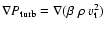
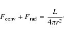
Assuming spherical symmetry we may write the equation of hydrostatic equilibrium:
 |
(1) |
 being the total pressure,
the matter density, G Newton's constant
of gravity, and
being the total pressure,
the matter density, G Newton's constant
of gravity, and  the stellar
mass inside radius r.
We neglect the atmospheric mass in comparison with the total stellar mass M,
and thus assume
the stellar
mass inside radius r.
We neglect the atmospheric mass in comparison with the total stellar mass M,
and thus assume
 .
For
.
For
 we have
 |
(2) |
where
and
 are the gas pressure and turbulent pressure, respectively,
and the last term is the force exerted by the radiation,
are the gas pressure and turbulent pressure, respectively,
and the last term is the force exerted by the radiation,
 |
(3) |
where  is the radiative energy flux per wavelength unit,
 and
and
 are the monochromatic absorption and
scattering coefficients, respectively, and c is the speed of light. The boundary condition for
Eq. (2) is
are the monochromatic absorption and
scattering coefficients, respectively, and c is the speed of light. The boundary condition for
Eq. (2) is
 |
(4) |
The formulation of the boundary condition involving the radiative force is,
however, not quite trivial in practice; see Plez et al. (1992).
For the turbulent pressure
one may write
 |
(5) |
where
is the gas density and  a characteristic velocity.
This pressure is measuring the force produced by the
kinetic movements of the gas, whether due to convective or other turbulent gas
motions. The parameter
a characteristic velocity.
This pressure is measuring the force produced by the
kinetic movements of the gas, whether due to convective or other turbulent gas
motions. The parameter  is
is  1, with an exact value depending on
whether the motions occur more or less isotropically. With our general lack of
knowledge about
it is reasonable to adopt an approximate recipe
for
.
We begin with assuming a depth independent value of .
The dominant depth variation in
1, with an exact value depending on
whether the motions occur more or less isotropically. With our general lack of
knowledge about
it is reasonable to adopt an approximate recipe
for
.
We begin with assuming a depth independent value of .
The dominant depth variation in
 ,
,
 being the gas constant,
occurs in .
Neglecting the variation in the temperature T and in the mean molecular weight
being the gas constant,
occurs in .
Neglecting the variation in the temperature T and in the mean molecular weight
 as well as in
and in
,
one finds
as well as in
and in
,
one finds
 |
(6) |
where
 is the flux-weighted mean of the extinction coefficient per gram
and L the luminosity of the star. Here, we have also assumed that the dominating fraction
of the stellar flux is carried by radiation, i.e. the approximation is most accurate for
the upper radiative zones of the models.
One may regard the right-hand side of Eq. (6) as the
local effective surface gravity
is the flux-weighted mean of the extinction coefficient per gram
and L the luminosity of the star. Here, we have also assumed that the dominating fraction
of the stellar flux is carried by radiation, i.e. the approximation is most accurate for
the upper radiative zones of the models.
One may regard the right-hand side of Eq. (6) as the
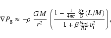
local effective surface gravity
 times .
We thus find that we can mimic the
effects of the radiative force and/or the turbulent pressure on the models by using
models with those effects neglected with an adjusted gravity:
times .
We thus find that we can mimic the
effects of the radiative force and/or the turbulent pressure on the models by using
models with those effects neglected with an adjusted gravity:
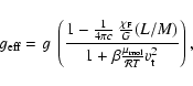 |
(7) |
where
 |
(8) |
Defining the effective
Eddington luminosity,
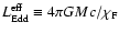 ,
we obtain
,
we obtain
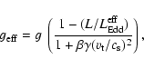 |
(9) |
where
 is the sound spead
for an ideal gas and
is the sound spead
for an ideal gas and  is the adiabatic
index. Basically, we have neglected the depth variation in
is the adiabatic
index. Basically, we have neglected the depth variation in
 in deriving this expression.
Thus, a model with a turbulent velocity
may be represented by a
model with a reduced gravity
and
 ,
according to
this recipe.
Similarly, effects
from the radiation force may be mimicked by changes in g or M.
However, the
Planck mean may vary strongly with depth and with stellar fundamental
parameters, and one should therefore be careful in the use of Eq. (7)
for exploring the radiative effects on the atmospheric structure and, e.g., the
possible effects on mass-loss rates. For a more detailed study for red
supergiants and asymptotic-branch stars, see Gustafsson & Plez (1992) and
Jørgensen & Johnson (1992), respectively.
We have tested the use of Eq. (7) to simulate
the effects of turbulent pressure for a number of models at various points in
the grid and find that it leads to very small errors in the temperature
structure (less than 5 K in the temperature throughout the model for
a depth independent
,
according to
this recipe.
Similarly, effects
from the radiation force may be mimicked by changes in g or M.
However, the
Planck mean may vary strongly with depth and with stellar fundamental
parameters, and one should therefore be careful in the use of Eq. (7)
for exploring the radiative effects on the atmospheric structure and, e.g., the
possible effects on mass-loss rates. For a more detailed study for red
supergiants and asymptotic-branch stars, see Gustafsson & Plez (1992) and
Jørgensen & Johnson (1992), respectively.
We have tested the use of Eq. (7) to simulate
the effects of turbulent pressure for a number of models at various points in
the grid and find that it leads to very small errors in the temperature
structure (less than 5 K in the temperature throughout the model for
a depth independent  in the interval 0 to 10 km s-1).
We, therefore, have chosen to set
for all grid models, and advise those
who would have liked a different choice to use models with a different mass
or g, according to the recipe given in Eq. (7). It should be noted that
the mixing-length treatment of convection adopted here (see Sect. 2.2 below)
leads to a rapidly varying formal convective velocity, in particular close to
the boundary where Schwarzschild stability sets in. If this variation were included
the term
in the interval 0 to 10 km s-1).
We, therefore, have chosen to set
for all grid models, and advise those
who would have liked a different choice to use models with a different mass
or g, according to the recipe given in Eq. (7). It should be noted that
the mixing-length treatment of convection adopted here (see Sect. 2.2 below)
leads to a rapidly varying formal convective velocity, in particular close to
the boundary where Schwarzschild stability sets in. If this variation were included
the term
 would get
a major contribution from
would get
a major contribution from
 .
However, more realistic simulations
of convection show that
varies much less with depth than ,
in
accordance with what was
assumed in the derivation of Eq. (7) above.
.
However, more realistic simulations
of convection show that
varies much less with depth than ,
in
accordance with what was
assumed in the derivation of Eq. (7) above.
The acceleration of gravity, g, for our spherical models is a depth-varying quantity, according
to Eq. (8). Also the stellar energy flux F(r) and
are varying with depth. Thus, we have
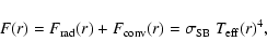 |
(10) |
where
 and
and
 are the radiative and convective flux, respectively, and
 is Stefan-Boltzmann's constant.
What remains constant (in stationary models) is the mass M (since only a tiny fraction of
the total stellar mass resides in the atmosphere), and the luminosity,
is Stefan-Boltzmann's constant.
What remains constant (in stationary models) is the mass M (since only a tiny fraction of
the total stellar mass resides in the atmosphere), and the luminosity,
 .
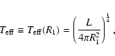
We label the models by the values of
and g at a radius
.
We label the models by the values of
and g at a radius
 where
where
 ,
the optical-depth scale based on the Rosseland mean opacity, is equal to 1.0, i.e.:
,
the optical-depth scale based on the Rosseland mean opacity, is equal to 1.0, i.e.:
 |
(11) |
 |
(12) |
We have used the version of the mixing-length ``theory'' as presented by
Henyey et al. (1965).
The convective energy flux is given by
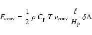 |
(13) |
Here,
 |
(14) |
where
 |
|
|
(15) |
 |
|
|
(16) |
and  is the local pressure scale height,
 |
(17) |
In the above,
 is the adiabatic temperature gradient;
  the specific heat at constant
pressure;
the specific heat at constant
pressure;
 the Rosseland
mean opacity; and
the Rosseland
mean opacity; and  the mixing
length. Equation (13) is valid if
the mixing
length. Equation (13) is valid if
 Also,
Also,
 |
(18) |
with
 |
(19) |
the derivative taken at constant thermodynamic pressure.
In addition to the mixing length parameter,
 ,
there are
two more explicit parameters in this formulation: y, which is related to the
adopted temperature distribution within the convective elements, and
,
there are
two more explicit parameters in this formulation: y, which is related to the
adopted temperature distribution within the convective elements, and  ,
which
deals with the energy dissipation by the turbulent viscosity. As a standard,
we have chosen the parameters according to the suggestions by Henyey et al.:
,
which
deals with the energy dissipation by the turbulent viscosity. As a standard,
we have chosen the parameters according to the suggestions by Henyey et al.:
 ,
y = 0.076 and
,
y = 0.076 and  .
It should be noted that different
choices than these are made, sometimes without being pointed out, in other
current work. The effects of varying the convective parameters were explored
for models of red giants by Gustafsson et al. (1975).
However, these
variations do not at all map the real possible range of errors due to our (inadequate)
treatment of the convective energy transport and do not give relevant
information on the effects of the thermal inhomogeneities generated by
convection.
The convective flux is added to the radiation energy flux,
and we may then write the energy equilibrium equation
.
It should be noted that different
choices than these are made, sometimes without being pointed out, in other
current work. The effects of varying the convective parameters were explored
for models of red giants by Gustafsson et al. (1975).
However, these
variations do not at all map the real possible range of errors due to our (inadequate)
treatment of the convective energy transport and do not give relevant
information on the effects of the thermal inhomogeneities generated by
convection.
The convective flux is added to the radiation energy flux,
and we may then write the energy equilibrium equation
 |
(20) |
All number densities of all atoms and molecules are assumed to follow from the
corresponding laws for thermal equilibrium; the Saha equation; and the
corresponding equation of chemical equilibrium for molecules
(Gibson & Heitler 1928; see also Russell 1934). Similarly,
all excitation equilibria and all partition functions are calculated adopting
the Boltzmann distribution, with higher terms in the atomic partition
functions cut according to the method of Irwin (1981).
The radiation source function is assumed to be
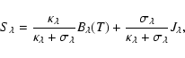 |
(21) |
where
 is the Planck function.
All line absorption is assumed to occur in true absorption, i.e.,
is the Planck function.
All line absorption is assumed to occur in true absorption, i.e.,
 |
(22) |
where
 and
and
 are the sums
of all continuous absorption contributions and line absorption contributions,
respectively. The mean intensity
are the sums
of all continuous absorption contributions and line absorption contributions,
respectively. The mean intensity  is calculated from
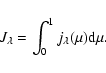 |
(23) |
Here, following Feautrier (1964), we define
 as
as
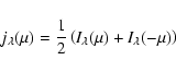 |
(24) |
where
 is the specific intensity in the direction specified by
 ,
,
 being the angle relative to a stellar radius.
The equation of radiative transfer for
being the angle relative to a stellar radius.
The equation of radiative transfer for  is
is
 |
(25) |
where
 is measured along the ray. For a discussion of adequate
boundary conditions for
and their implementation, see Nordlund (1984).
Knowing
,
the wavelength-integrated flux in the radial direction
can be calculated from a derivative of the second Eddington moment
is measured along the ray. For a discussion of adequate
boundary conditions for
and their implementation, see Nordlund (1984).
Knowing
,
the wavelength-integrated flux in the radial direction
can be calculated from a derivative of the second Eddington moment  ,
defined by
,
defined by
 |
(26) |
Thus, we have for the monochromatic flux
 |
(27) |
cf., Mihalas (1978, his Eq. (2.80)) and then
 |
(28) |
which is used in the energy conservation equation, Eq. (20).
Alternatively, the energy balance may be expressed as
 |
(29) |
For
 ,
which is often the case in the upper layers of the models, this is equivalent to
,
which is often the case in the upper layers of the models, this is equivalent to
![\begin{displaymath}
\int \kappa_\lambda~ \left[J_\lambda(\tau_{\rm Ross}) -
B_\l...
...\right]~ {\rm d}\lambda =
q_{\rm rad} - q_{\rm thermal} = 0,
\end{displaymath}](/articles/aa/full/2008/30/aa09724-08/img133.gif) |
(30) |
with
| |
|
 |
|
| |
|
 |
(31) |
The volume of physical data needed in the calculation of model atmospheres of
late-type stars is considerable. Data are needed for the calculation of the
ionisation equilibrium of atoms and the dissociation equilibrium of molecules.
These data include chemical composition data, ionisation energies
and dissociation energies, as well as
partition functions. Moreover, continuous absorption and scattering
coefficients are needed.
The, by far, most extensive and most demanding need, however,
is the various data that are necessary for the proper calculation of the line
absorption. Here, we shall briefly present the data used to calculate
ionisation-dissociation equilibria as well as continuous absorption and
scattering.
Some more details concerning the line-absorption data
are given in Papers II-VII.
The basic chemical composition adopted is that of the Sun, as listed by
Grevesse et al. (2007). There is still some dispute on the
C, N, and O abundances adopted there (C = 8.39, N = 7.78, and O = 8.66) and, therefore,
we have taken the data of Grevesse & Sauval (1998) with
CNO abundances higher by about 0.2 dex for an alternative solar-metallicity sub-grid. The effects of these differences are explored
in Sect. 6.3. In varying the overall metallicity of the models ([Me/H]), we have as a standard
scaled the abundances of all elements heavier than He in unison. The abundances of so-called elements O, Ne, Mg, Si, S, Ar, Ca, and Ti tend to vary somewhat differently for
galactic stars (see, e.g., Edvardsson et al. 1993;
Reddy et al. 2003;
Ryde & Lambert 2004; Nissen et al. 2004;
Cayrel et al. 2004). The variation, however,
is not necessarily the same for all stellar populations in the Galaxy
(see, e.g., Fuhrmann 1998; and Bensby et al. 2005) or in other galaxies
(see Venn et al. 2004). Therefore, we offer models with two different
sets of abundances: a set with a uniform scaling for each element with [Me/H]; and a set
where the elements have been scaled as follows: [/Fe] = 0.4 for
![$-5.0\le\rm [Me/H]\le -1.0$](/articles/aa/full/2008/30/aa09724-08/img136.gif) ;
[/Fe] =
;
[/Fe] =
![$-0.4\times \rm [Me/H]$](/articles/aa/full/2008/30/aa09724-08/img137.gif) for
for
![$-1.0 \le\rm [Me/H]\le 0.0$](/articles/aa/full/2008/30/aa09724-08/img138.gif) ;
and
[/Fe] = 0.0 for [Me/H]
;
and
[/Fe] = 0.0 for [Me/H]  0.0. For the giant stars, the results of the first dredge up
of CNO processed material is known to lead to a reduced carbon abundance and a correspondingly
increased N abundance (cf. e.g., Boothroyd & Sackmann 1999). We therefore also offer models with revised C and N such that
C/N = 1.5 and 0.5 by number, respectively, as alternatives to the solar value of C/N = 4.07,
though keeping C+N constant (cf. Sect. 6.3). For the corresponding giant stars, the changed C/N ratio is usually
accompanied by a decrease in the isotopic ratio 12C/13C. For the
``CN processed'' models we have
therefore changed this ratio from solar to 20 and 4, respectively. Finally, we also present models with increased
C abundances for the M stars and carbon stars such that
C/O ranges from 0.54 to 0.99 (M and S star models) to above 1.0 (models for
C stars).
0.0. For the giant stars, the results of the first dredge up
of CNO processed material is known to lead to a reduced carbon abundance and a correspondingly
increased N abundance (cf. e.g., Boothroyd & Sackmann 1999). We therefore also offer models with revised C and N such that
C/N = 1.5 and 0.5 by number, respectively, as alternatives to the solar value of C/N = 4.07,
though keeping C+N constant (cf. Sect. 6.3). For the corresponding giant stars, the changed C/N ratio is usually
accompanied by a decrease in the isotopic ratio 12C/13C. For the
``CN processed'' models we have
therefore changed this ratio from solar to 20 and 4, respectively. Finally, we also present models with increased
C abundances for the M stars and carbon stars such that
C/O ranges from 0.54 to 0.99 (M and S star models) to above 1.0 (models for
C stars).
We use the atomic partition functions and ionisation energies from
Irwin (1981) with some modifications.
The molecular equilibria were calculated using
the partition functions and dissociation energies of Sauval (private
communication), which is an update of Sauval & Tatum (1984) for diatomic molecules, and Irwin (1988, and private communication) for polyatomic molecules.
Altogether 519 molecules were included in the equilibrium calculations.
A comparison with equilibria calculated by Piskunov (private communication)
shows a very good agreement.
The continuous absorption from
H I, H-, H2-, H2+, He I, He-, C I,
C II, C-, N I, N II, N-, O I, O II,
O-, Mg I, Mg II, Al I, Al II, Si I,
Si II, Ca I, Ca II, Fe I, and Fe II,
as well as CH, OH, CO-, and H2O- were calculated from sources,
according to Table 1.
Table 1:
Sources of data for continuous opacities.
Corrections were made to the data for
C I, Mg I, Al I, Si I to account for
the fact that TOP base photon cross sections are published with theoretical
energy levels derived from the model atom, which depart significantly from
the much better known data from laboratory work. For these four species,
corrections were considered necessary since they significantly
affect the UV fluxes of the models. We identified the individual TOP base energy levels for these species
and shifted them to the empirical energies given by the National Institute of Standards
and Technology (NIST) data base (http://physics.nist.gov/PhysRefData/ASD/index.html).
The TOP base gives the photon absorption cross section (in Mbarn) as a
function of the energy of the ejected electron.
This electron energy was converted to the energy of the absorbed photon by
adding the ionisation energy from the specific electronic level.
The cross-section data for all levels was summed up, assuming LTE for a
number of temperatures, and plotted at the full original wavelength
resolution at different temperatures.
Also collision-induced absorption of H I+H I, H I+He I,
H2 + H I,
H2 + H2, and H e I was included.
H
e I was included.
H and H
and H
 CIA data from Borysow et al., referred to in
Table 1, are
available from http:www.stella.nbi.dk/pub/scan. More extensive data
sets for the CIA are publicly accessible from http://www.astro.ku.dk/~aborysow.
Continuous electron scattering as well as Rayleigh scattering from H I,
H2 and He I was included and assumed to be isotropic.
CIA data from Borysow et al., referred to in
Table 1, are
available from http:www.stella.nbi.dk/pub/scan. More extensive data
sets for the CIA are publicly accessible from http://www.astro.ku.dk/~aborysow.
Continuous electron scattering as well as Rayleigh scattering from H I,
H2 and He I was included and assumed to be isotropic.
Line absorption data for atoms and first ions were originally adopted from VALD-1
(Piskunov et al. 1995), but recently data for the ten most important species were
modified according to VALD-2 (Stempels et al. 2001).
The updated species are Si I, Ca I, Ca II, Ti II,
Cr I, Cr II, Mn II, Fe I, Fe II, and
Ni II. The VALD-data adopted include the very numerous line data
calculated by Kurucz & Bell (1995, see also
http://kurucz.harvard.edu), including lines
between predicted energy levels that are not yet experimentally verified.
The gf values were, however, modified for
948 lines from VALD-1 and 1276 lines from VALD-2 in the wavelength
range 3783 to 8968 Å, based on fits of synthetic solar intensity spectra. These model spectra were
calculated with the Holweger & Müller (1974) model and compared with the observed solar
disk-centre FTS spectrum of Brault & Neckel (1987), see Paper II.
The model spectrum was required to match the observed equivalent widths to within 0.1 dexin log gf. The
resulting gf values are listed at http://marcs.astro.uu.se.
Line absorption data for diatomic and polyatomic molecules were
considered for species according to Table 2. Most line lists of Jørgensen and collaborators are described
by Jørgensen (1997) and may be obtained by anonymous ftp via
www.stella.nbi.dk/pub/scan.
Line lists for HCN, C2H2 and C3 will be added to this data base later in connection with the paper on carbon-enriched
stars in the present series.
The line lists of
Plez referred to in Table 2 as ``unpublished'' are available via
http://marcs.astro.uu.se.
Some of these lists were especially
tailored for the present grid; in such cases a more detailed description of
the line list for the particular species is to be found in one of the
subsequent papers in the present series. For the OH A-X system we did not use the data of Gillis et al. (2001)
since the Kurucz (1995b) list includes higher vibration and rotation states.
For MgH we did not include the new data of Skory et al. (2003) for 24MgH
since we were anxious to be consistent with the MgH lines for other Mg isotopes.
Hydrogen line and bound-free opacity, and their merging,
were modelled using a code by Barklem (http://www.astro.uu.se/~barklem/hlinop.html), which is based on
the occupation probability formalism of Däppen et al. (1987). The details of the description
of this line opacity are given by Barklem & Piskunov (2003).
For the atomic lines of metals, the damping
wings were also calculated, using the
best available data (Anstee & O'Mara 1995;
Barklem et al. 2000a, and references therein, 2000b;
Barklem & Aspelund-Johansson 2005; and Barklem, private communication).
For weak lines where such data were missing we just adopted the Unsöld recipe
(cf., Unsöld 1955, his Eq. (76.43)),
with a constant enhancement factor set to 2.0 for Na I, 1.3 for
Si I, 1.8 for Ca I, 1.4 for Fe I
and 2.5 for all other species. (The damping constants given in the line list
of Kurucz, which were obtained by perturbation theory, might have been preferred to the use of
Unsöld values.)
For the molecules, damping was not taken into account - the lack of proper
damping parameters makes any such attempt questionable. Also, the huge density of
molecular lines often makes the damping wings of a line less important since the
intensity of the Doppler cores of neighbouring lines dominate.
In general, it should be noted that although the present atomic and molecular data are very extensive,
and much more complete and accurate than, e.g., a decade ago, they are far from perfect. Considerable improvements
are still needed, both by adding many more faint lines and by determining line strengths more accurately. The risk
that present models are still underblanketed must be appreciated.
Table 2:
Sources of data for molecular line opacities.
Equations (1)-(3), (13),
(20) or (30), (27), and (28) with relevant boundary conditions
form a closed system of equations for determining the dependent variables
,
T, ,
 ,
,
,
as well as quantities like
,
,
,
as well as quantities like
 ,
,
or alternatively
,
,
or alternatively
 .
In addition to these quantities, we also need
to calculate quantities characteristic (in LTE at least) of the local
temperature and pressure:
.
In addition to these quantities, we also need
to calculate quantities characteristic (in LTE at least) of the local
temperature and pressure:
 ,
,
 ,
,
Q,
and .
The system of equations is solved on a
scale,
with
,
,
Q,
and .
The system of equations is solved on a
scale,
with
 calculated by integration over all 105 wavelength
points. This choice of depth scale leads to temperature structures that are
only moderately affected by changes in the fundamental stellar parameters. Basically,
a standard multi-dimensional Newton-Raphson method is applied to solve the highly non-linear
system. All equations are first
discretised, in the variables
and
calculated by integration over all 105 wavelength
points. This choice of depth scale leads to temperature structures that are
only moderately affected by changes in the fundamental stellar parameters. Basically,
a standard multi-dimensional Newton-Raphson method is applied to solve the highly non-linear
system. All equations are first
discretised, in the variables
and  .
Next, all the resulting
equations are linearized in the dependent variables listed above. The input variables
at the calculation of thermodynamic quantities and absorption coefficients are T and ,
which is a very appropriate choice as long as H- is a dominating opacity source. (For the coolest models, e.g.,
.
Next, all the resulting
equations are linearized in the dependent variables listed above. The input variables
at the calculation of thermodynamic quantities and absorption coefficients are T and ,
which is a very appropriate choice as long as H- is a dominating opacity source. (For the coolest models, e.g.,  or
could have been
more advantageous.) As a result
of the linearisation, a set of linear equations in the variations of the dependent variables
is obtained. The coefficients of this system contain derivatives of a great
number of quantities relative to the dependent variables. First, a starting
model is adopted to make a first calculation of the coefficients possible.
Next, the system of linear equations is solved numerically, the resulting
variations are applied to the dependent variables, new coefficients are
calculated, and a new solution is obtained for the variations.
The elimination scheme is basically that of Rybicki (1971), also applied
by Gustafsson & Nissen (1972) and Gustafsson et al. (1975), with an elimination work
that scales linearly with the number of wavelength points,
or
could have been
more advantageous.) As a result
of the linearisation, a set of linear equations in the variations of the dependent variables
is obtained. The coefficients of this system contain derivatives of a great
number of quantities relative to the dependent variables. First, a starting
model is adopted to make a first calculation of the coefficients possible.
Next, the system of linear equations is solved numerically, the resulting
variations are applied to the dependent variables, new coefficients are
calculated, and a new solution is obtained for the variations.
The elimination scheme is basically that of Rybicki (1971), also applied
by Gustafsson & Nissen (1972) and Gustafsson et al. (1975), with an elimination work
that scales linearly with the number of wavelength points,
 .
.
The total radiative flux,
,
and
 are non-local functionals of the
model structure and can be calculated from a solution of the transfer
equation, Eq. (25).
For the model structure obtained after each iteration, we need an accurate
solution of the equation with the source function
are non-local functionals of the
model structure and can be calculated from a solution of the transfer
equation, Eq. (25).
For the model structure obtained after each iteration, we need an accurate
solution of the equation with the source function
 given by Eqs. (21) and (23), which then enables us to
calculate
and
for that structure.
These quantities are used to calculate the corrections (right hand sides) in the
next Newton-Raphson iteration.
We also need a linearisation of
and
in T and
to calculate factors, symbolically written as, e.g.,
given by Eqs. (21) and (23), which then enables us to
calculate
and
for that structure.
These quantities are used to calculate the corrections (right hand sides) in the
next Newton-Raphson iteration.
We also need a linearisation of
and
in T and
to calculate factors, symbolically written as, e.g.,
 ,
or
,
or
 ,
to be used in the
coefficient matrix in the forth-coming iteration.
Here,
,
to be used in the
coefficient matrix in the forth-coming iteration.
Here,  and
and  are any two radial optical depths in the stellar
atmosphere. I.e., we need to estimate how the radiation
contribution to the energy balance at each point in the atmosphere is affected
by variations in temperature or pressure anywhere else. Both these tasks are
accomplished with the iterative method of Nordlund (1984), which was applied to
model atmosphere calculations by Plez et al. (1992) for M giants
and by Jørgensen et al. (1992) for carbon stars. Here, we shall
only give a brief summary for reference.
are any two radial optical depths in the stellar
atmosphere. I.e., we need to estimate how the radiation
contribution to the energy balance at each point in the atmosphere is affected
by variations in temperature or pressure anywhere else. Both these tasks are
accomplished with the iterative method of Nordlund (1984), which was applied to
model atmosphere calculations by Plez et al. (1992) for M giants
and by Jørgensen et al. (1992) for carbon stars. Here, we shall
only give a brief summary for reference.
 |
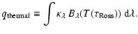
Figure 1:
Sketch of the geometric representation used for solving the spherically-symmetric radiative transfer problem.
The full radius mesh used for representing the variables as functions of radius (about 7 points
per decade in
 )
is indicated along the radius vector by a set of concentric circles. The distance of rays from
the centre of symmetry is measured by the impact parameter p. About 15 rays with impact parameters )
is indicated along the radius vector by a set of concentric circles. The distance of rays from
the centre of symmetry is measured by the impact parameter p. About 15 rays with impact parameters   ,
the core radius, are used and are represented here by two dashed lines. The set of rays that do not hit the core,
typically about 50 rays but dependent of wavelength, are here represented by five parallel rays. The mesh of points used for solving the
equation of radiative transfer are the crossing points between the circles and the horizontal lines. Distances along the rays are
measured by ,
the core radius, are used and are represented here by two dashed lines. The set of rays that do not hit the core,
typically about 50 rays but dependent of wavelength, are here represented by five parallel rays. The mesh of points used for solving the
equation of radiative transfer are the crossing points between the circles and the horizontal lines. Distances along the rays are
measured by  where
where
 . . |
| Open with DEXTER |
The equation of radiative
transfer is solved along a set of parallel rays, which cover a suitable range
of impact parameters, chosen individually for each wavelength
(cf. Fig. 1).
In practice,
about 15 rays equidistant in  (the cosine of the angle relative to the
normal) are chosen for impact parameters <,
where
is
the radius for the stellar non-transparent ``core''. This core is defined by a radial
(the cosine of the angle relative to the
normal) are chosen for impact parameters <,
where
is
the radius for the stellar non-transparent ``core''. This core is defined by a radial
 ,
to allow a great enough thermalization depth for scattered light.
Rays that never hit this core, but
only pass through the transparent
``atmospheric'' region, are all chosen to go through pre-selected
points in the vertical scale along a line through the stellar
centre and perpendicular to the ray. These rays are distributed with about
5 rays per decade in
along this line.
,
to allow a great enough thermalization depth for scattered light.
Rays that never hit this core, but
only pass through the transparent
``atmospheric'' region, are all chosen to go through pre-selected
points in the vertical scale along a line through the stellar
centre and perpendicular to the ray. These rays are distributed with about
5 rays per decade in
along this line.
Scattering is handled by an iterative technique where the radiative transfer
equation along a particular single ray is used to correct residual errors.
This technique uses a ``form factor''  ,
,
 |
(32) |
Here, both
and
can be taken from the previous iteration,
since their ratio is not very dependent on the detailed shape of the source
function; in this respect, the method is analogous to the variable Eddington
technique of Auer & Mihalas (1970) in handling the angular dependence of the
radiative field. After a few iterations a correct solution is obtained.
When linearising the energy equilibrium equation (Eqs. (20) or (30)) we linearise the transfer equation along a representative ray and apply the
form factor, as calculated in the preceding iteration. This relates the
changes in the energy balance to changes of the specific intensity along the
ray. We adopt this relation as typical for all rays. The final result is then
a coupling of the energy equilibrium at each point in the atmosphere to
temperatures and electron pressures all over the model.
The representative ray
is chosen in the following way: at the radius in the discretisation of the
scale where
,
measured radially is about
 the set of rays hits
the sphere at a set of angles relative to the normal. We take the ray where the
cosine for this angle is close to
the set of rays hits
the sphere at a set of angles relative to the normal. We take the ray where the
cosine for this angle is close to
 ,
a natural choice in
view of the result of the Eddington approximation that the outgoing intensity
from a gray atmosphere with a linear source function in this direction
has a characteristic depth of formation which can be taken as an average depth of
formation for all disk rays.
,
a natural choice in
view of the result of the Eddington approximation that the outgoing intensity
from a gray atmosphere with a linear source function in this direction
has a characteristic depth of formation which can be taken as an average depth of
formation for all disk rays.
In order to obtain a sufficient numerical accuracy we
linearise the radiative flux directly (Eq. (20)) only for optical depths
 ,
while for smaller depths we linearise the divergence
of the flux (i.e. Eq. (30)).
This avoids the loss of accuracy associated with the nearly
constant monochromatic fluxes at most wavelengths in the optically thin layers.
In the discretisation in
we use 56 points,
distributed between
,
while for smaller depths we linearise the divergence
of the flux (i.e. Eq. (30)).
This avoids the loss of accuracy associated with the nearly
constant monochromatic fluxes at most wavelengths in the optically thin layers.
In the discretisation in
we use 56 points,
distributed between
 and
and
 .
.
The integrals over
are calculated using the trapezian rule.
In the discretisation, we use 10 000 points during the first
iterations.
In the final iterations there are 108 000 points, set to produce a sampling density
 ,
with
,
with
 Å for models warmer than 3500 K and
1300 Å for cooler models, and
Å for models warmer than 3500 K and
1300 Å for cooler models, and
 .
We have made a series of numerical experiments to investigate the errors
resulting from the sampling of the spectrum with a resolution smaller than
what corresponds to the characteristic line widths. We did this investigation
by making a number of models, each with 30 000 wavelength points. The models were
identical, except for the particular wavelength points which were sampled differently.
We then found the temperature errors for
.
We have made a series of numerical experiments to investigate the errors
resulting from the sampling of the spectrum with a resolution smaller than
what corresponds to the characteristic line widths. We did this investigation
by making a number of models, each with 30 000 wavelength points. The models were
identical, except for the particular wavelength points which were sampled differently.
We then found the temperature errors for
 to be less than
 K with the maximum errors in the upper
layers of the model (above
K with the maximum errors in the upper
layers of the model (above
 ). The corresponding errors in the
flux integrals and flux derivative integrals (i.e., the integrals in Eqs. (28) and (30))
by the sampling procedure are less than 1.5%. For the grid models with
108 000 wavelength points, the sampling errors are correspondingly smaller
(by approximately a factor of
(108 000/30 000)-1/2). They then lead to
temperature errors of about
). The corresponding errors in the
flux integrals and flux derivative integrals (i.e., the integrals in Eqs. (28) and (30))
by the sampling procedure are less than 1.5%. For the grid models with
108 000 wavelength points, the sampling errors are correspondingly smaller
(by approximately a factor of
(108 000/30 000)-1/2). They then lead to
temperature errors of about
 K or less.
For the M and C star models, we have found the corresponding errors in fluxes and
temperatures to be reduced by a factor of three or more. This is a result of the
overlapping molecular-line absorption, which reduces the dominance of a few
strong metal lines in the flux derivative integrals in the
upper model layers, lines which otherwise demand a high density of sampling points if
no special measures are taken to cover them properly by quadrature points.
K or less.
For the M and C star models, we have found the corresponding errors in fluxes and
temperatures to be reduced by a factor of three or more. This is a result of the
overlapping molecular-line absorption, which reduces the dominance of a few
strong metal lines in the flux derivative integrals in the
upper model layers, lines which otherwise demand a high density of sampling points if
no special measures are taken to cover them properly by quadrature points.
It should be noted that
the fluxes, even if they are monochromatically precise within the model
constraints, may be far from representative for the regions surrounding each
wavelength point in the spectrum. Thus, model fluxes integrated to represent
narrow spectral regions,
 wide, will have relative errors
of typically
wide, will have relative errors
of typically
![$0.3\times[\lambda/(R \Delta \lambda)]^{1/2}$](/articles/aa/full/2008/30/aa09724-08/img189.gif) .
E.g., for 100 Å wide bands
at 5000 Å, the sampling errors will correspond to standard deviations of typically 1.6%.
Obviously, synthetic spectra more detailed than the model fluxes must be calculated
for theoretical calibrations of, e.g., narrow-band photometry. We have included the surface
fluxes in all 108 000 wavelength points into the model files
published on http://marcs.astro.uu.se - more detailed high-resolution synthetic
spectra will also be gradually added.
.
E.g., for 100 Å wide bands
at 5000 Å, the sampling errors will correspond to standard deviations of typically 1.6%.
Obviously, synthetic spectra more detailed than the model fluxes must be calculated
for theoretical calibrations of, e.g., narrow-band photometry. We have included the surface
fluxes in all 108 000 wavelength points into the model files
published on http://marcs.astro.uu.se - more detailed high-resolution synthetic
spectra will also be gradually added.
For the integration of the
moments of the radiative intensity (in
practice )
we use the points defined by the angles in the crossing points between
the different parallel rays with impact parameter pi and the concentric spheres
around the stellar centre with radii rk corresponding to the discretisation of the
vertical
scale,
cf. Fig. 1.
I.e.,
 ,
directions for which
is directly available. Considering the
character of the radiation field in a spherical atmosphere, this is an adequate
set of
points. This, despite the fact that they are different for different
radii and different wavelengths. The typical number of
points is 6 in
the plane-parallel case and typically 40-60 in the spherical models.
The quadrature in
is performed using piece-wise cubic splines, as described
by Nordlund (1984).
,
directions for which
is directly available. Considering the
character of the radiation field in a spherical atmosphere, this is an adequate
set of
points. This, despite the fact that they are different for different
radii and different wavelengths. The typical number of
points is 6 in
the plane-parallel case and typically 40-60 in the spherical models.
The quadrature in
is performed using piece-wise cubic splines, as described
by Nordlund (1984).
The line opacities have been pretabulated in the following way: for each
individual species (e.g. H I, C I, C II, CH, C2, etc.) and the full
set of wavelength
points, arrays of line absorption were calculated for a number of T-P6 points
(or T points for the molecules).
The value of P6 is given by
 |
(33) |
where the static dipole polarisabilities and mean velocities of He I and H2relative to that of H I
have been used to approximately scale the broadening for H I to these species.
Altogether, 17 T values and 18 P6 values were chosen. Tables were
constructed for 6 different values of the microturbulence parameter,
 ,
1, 2, 5, 10, and 20 km s-1.
Next, for a given chemical composition and microturbulence parameter,
the tables were summed for
all atoms and ions over the different species with due consideration to the
ionisation equilibria. This gave one table of the summed atomic
line absorption at each lambda point for each T, P6, and
,
1, 2, 5, 10, and 20 km s-1.
Next, for a given chemical composition and microturbulence parameter,
the tables were summed for
all atoms and ions over the different species with due consideration to the
ionisation equilibria. This gave one table of the summed atomic
line absorption at each lambda point for each T, P6, and
 chosen.
For each molecular species we produced a table for a combination of
12 T and 6
values.
In the subsequent model-atmosphere calculations, we found the logarithmic line absorption
coefficients from these tables by spline interpolation
to the appropriate temperatures and logarithmic pressures.
(If models are needed at microturbulence parameters different from
those of the tables, interpolation can be made.)
chosen.
For each molecular species we produced a table for a combination of
12 T and 6
values.
In the subsequent model-atmosphere calculations, we found the logarithmic line absorption
coefficients from these tables by spline interpolation
to the appropriate temperatures and logarithmic pressures.
(If models are needed at microturbulence parameters different from
those of the tables, interpolation can be made.)
In the calculation of opacity data tables,
we added the relevant absorption for each spectral line
at each T and P6 value to the table for wavelengths
points progressing to the blue and the red side of the central line wavelength
as far as the line opacity exceeded a predefined cross section. Also, for very weak lines, we
then included each line
at a minimum of two wavelength points.
To limit the total computing time needed and still guarantee that no significant opacity was lost,
these limiting cross sections were empirically determined for groups of
atoms and ions.
The total computing time needed for the calculation of a model
atmosphere (the pre-calculation of the absorption coefficient tables
excluded) scales approximately as follows: (1) for the radiative transfer
part of the problem the time is proportional to
 ;
(2) for the calculation of ionisation equilibria and molecular equilibria the time scales as
;
(2) for the calculation of ionisation equilibria and molecular equilibria the time scales as
 ;
and (3) for the calculation of absorption coefficients as
;
and (3) for the calculation of absorption coefficients as
 .
In addition, (4) some initiation time is needed. Setting
.
In addition, (4) some initiation time is needed. Setting
 ,
,
 and
and
 and noting that we usually set
  in
the plane-parallel case and that
in
the plane-parallel case and that
 in the spherical case, we find
empirically that the time
in the spherical case, we find
empirically that the time
 needed per iteration is, in seconds,
 |
(34) |
For a typical spherical model with 108 000 wavelength points about 80 s per iteration are needed
on a Mac Pro quad Intel Xeon 2.66 GHz computer for one processor.
For a plane-parallel model this is reduced to about
60 s. The relatively small reduction reflects the fact that interpolation in the line-absorption
tables (the
 term) constitutes a major fraction of the computing time; for
a highly spherical case (when
term) constitutes a major fraction of the computing time; for
a highly spherical case (when  becomes great) only, the radiative transfer calculations
dominate. No doubt, the calculations of absorption coefficients and their derivatives
could be sped up further, e.g., by pre-tabulation. This would primarily be of interest in the
calculation of extensive model grids, or for models with more complex physics than described by the
approximations in Sect. 3, e.g., with regard to hydrodynamics.
becomes great) only, the radiative transfer calculations
dominate. No doubt, the calculations of absorption coefficients and their derivatives
could be sped up further, e.g., by pre-tabulation. This would primarily be of interest in the
calculation of extensive model grids, or for models with more complex physics than described by the
approximations in Sect. 3, e.g., with regard to hydrodynamics.
In multi-dimensional Newton-Raphson schemes like the present one,
convergence is rapid, provided that a starting solution, which is
close enough to the final solution, has been chosen.
When model calculations are started from scratch with the MARCS program,
usually
a gray starting model is chosen for the radiative zone. When the
calculated flux in the convectively unstable zone of the first starting model exceeds the total flux, the
temperature gradient is automatically and directly reduced, beginning at the onset of
the convective instability until the convective flux is smaller
than the prescribed total flux. In the present
grid, we usually start from a nearby model in the fundamental-parameter
space. If the starting model has a different effective temperature, a
simple scaling of the temperature structure
 may be applied,
but this is not necessary if steps of only a few hundred K are taken in
.
may be applied,
but this is not necessary if steps of only a few hundred K are taken in
.
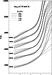 |
Figure 2:
The temperature structures for a set of model atmospheres with
different
,
log g = 3 and different metallicities. |
| Open with DEXTER |
The route towards convergence is often rapid, but not always quadratical.
The pronounced non-linearities, not the least in the temperature
dependencies of the molecular equilibria with strong effects
on the opacities may slow down the convergence if one is not very close
to the final solution. Also, the changing
presence and depth of the convective zone with temperature and metallicity
affect the convergence.
Usually, convergence to temperature corrections of
less than a few K, and logarithmic pressure corrections smaller than
0.01 dex, is obtained all through the models after 4 to 10 iterations. For models
with
 K, the convergence is close to quadratic with
corrections reduced by almost one order of magnitude from one iteration to the next.
For the cooler models the convergence is slower but still fast. For some
parameter choices, however, converged models were not obtained. In particular,
this is the case for models with a strong radiative pressure
gradient (i.e., close to the effective Eddington limit, see
Gustafsson & Plez 1992) which is close
to upsetting the hydrostatic equilibrium condition, i.e., models with high
temperatures and low gravities. Another difficulty occurs for models in a
small band in the
K, the convergence is close to quadratic with
corrections reduced by almost one order of magnitude from one iteration to the next.
For the cooler models the convergence is slower but still fast. For some
parameter choices, however, converged models were not obtained. In particular,
this is the case for models with a strong radiative pressure
gradient (i.e., close to the effective Eddington limit, see
Gustafsson & Plez 1992) which is close
to upsetting the hydrostatic equilibrium condition, i.e., models with high
temperatures and low gravities. Another difficulty occurs for models in a
small band in the
 diagram, extending from about
 ,
log g = 5, to
,
log g = 5, to
 ,
log g = 3, where convergence is not achieved in the deepest layers
of the models because the convectively unstable regions are swapping between thin
convective zones and zones extending to
depths below the bottom of the model. This difficulty may be circumvented
by extending the depth scale of the model to deeper layers. Some of the models, though not
fully converged in the deepest layers, are nevertheless presented in the grid
since the spectrum forming regions (above
,
log g = 3, where convergence is not achieved in the deepest layers
of the models because the convectively unstable regions are swapping between thin
convective zones and zones extending to
depths below the bottom of the model. This difficulty may be circumvented
by extending the depth scale of the model to deeper layers. Some of the models, though not
fully converged in the deepest layers, are nevertheless presented in the grid
since the spectrum forming regions (above
 )
are not affected
at all. Convergence problems occurred for some of the coolest models with H2 convection
zones at the surface as well as for models where the radiative pressure totally dominates the gas pressure.
)
are not affected
at all. Convergence problems occurred for some of the coolest models with H2 convection
zones at the surface as well as for models where the radiative pressure totally dominates the gas pressure.
All models of the grid will be accessible via http://marcs.astro.uu.se/. The organization of the model files is
described there. We give details of structures, thermodynamic variables,
molecular partial pressures, and fluxes in 105 wavelength points in the files.
In Fig. 2,
we present some sample temperature structures of grid models with different effective temperatures and metallicities.
It is seen that the variation with metallicity at the surface and in the deep layers
increases when
decreases from 8000 K
to 5000 K, and that this
variation with metallicity changes sign at 4000 K in a non-trivial way.
Subsequently, we will comment on this and other properties of the grid models. Our discussion here
is confined to general properties of the model structures, while more details on models of particular
types of stars, as well as discussion of model fluxes are deferred to later papers in this
series.
The effects of spectral lines on stellar atmospheres (``blanketing'') have been explored thoroughly since it became
possible to calculate models with lines included in the 1960s and 1970s. Here, we shall make a short summary
of these results as a background for some more specific comments on the blanketing effects in the new grid.
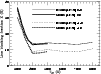 |
Figure 3:
The blocking fraction X in percent for models in the grid with two different metallicities.
The dwarf models all have log g=4.5 while the giant models
have log g values increasing with temperature, from log g=0.0 at
 K to log g=3.0 at K to log g=3.0 at
 K. K. |
| Open with DEXTER |
In general, the blocking of
radiation leads to heating of the deeper layers of the atmospheres (``back-warming''). Here and subsequently we measure the
back-warming effect at a given continuum optical depth, in practice at
 nm (i.e., not
,
which for the cooler models is strongly
affected by line absorption). The back-warming is in fact
easily estimated directly from the definition of the effective temperature
by assuming that a model with effective temperature
is heated such that the deeper layers
correspond to an unblanketed model with an effective temperature,
nm (i.e., not
,
which for the cooler models is strongly
affected by line absorption). The back-warming is in fact
easily estimated directly from the definition of the effective temperature
by assuming that a model with effective temperature
is heated such that the deeper layers
correspond to an unblanketed model with an effective temperature,
 |
(35) |
where X is the fraction of the integrated continuous
flux blocked out by spectral lines,
 |
(36) |
The validity of this relation has been tested for models with different
fundamental parameters by calculating X of these models, and then we constructed unblanketed models with effective temperatures
revised according to the relation. Next, we compared these models with the corresponding blanketed ones. The test came out
favourably - for models all over the parameter space of the grid, the
structures in the
interval
 were reproduced astonishingly well by the corresponding unblanketed ones;
the additional steepening of the temperature gradient across the
interval for the
blanketed model with solar abundances may typically amount to
were reproduced astonishingly well by the corresponding unblanketed ones;
the additional steepening of the temperature gradient across the
interval for the
blanketed model with solar abundances may typically amount to
 per decade in
.
per decade in
.
 |
Figure 4:
The effects of switching off line absorption on the temperature structure of a sequence of models with log g=3.0 and solar
metallicity. Note that
 .
It is seen that the blanketing effects are fairly independent of effective temperature for models
with .
It is seen that the blanketing effects are fairly independent of effective temperature for models
with
 |
| Open with DEXTER |
We also calculated the total blocking fraction X
for the grid models and find the remarkable behaviour shown in Fig. 3.
Thus, X stays nearly constant for the temperature interval
 K for a given metallicity, and
is closely identical for dwarfs and giants, while below 4000 K it increases as temperature goes down, due to the heavy TiO and H2O
blocking. Here, the metallicity sensitivity of X decreases while the gravity sensitivity increases. The decreasing metallicity
sensitivity reflects the fact that the molecular lines fill in the
continuum regions in the spectrum and define the
scale (
being rather robust against metallicity
changes).
K for a given metallicity, and
is closely identical for dwarfs and giants, while below 4000 K it increases as temperature goes down, due to the heavy TiO and H2O
blocking. Here, the metallicity sensitivity of X decreases while the gravity sensitivity increases. The decreasing metallicity
sensitivity reflects the fact that the molecular lines fill in the
continuum regions in the spectrum and define the
scale (
being rather robust against metallicity
changes).
For the upper layers of the atmospheres the situation is more complex,
as was discussed, e.g., by Gustafsson et al. (1975);
Gustafsson & Olander (1979); and Carbon (1979); and as is illustrated
in Fig. 4. In short, for LTE the spectral-line absorption may cause a cooling or a heating, depending on whether the absorption is located
on the long-wavelength side of the local Planck function (cooling, Case 1) or on the short-wavelength side. In the latter case,
heating (2a) or cooling (2b) may result, depending on whether the absorption is concentrated to the upper layers (2a) or
whether it extends to the deeper atmosphere (2b). Examples of Case 1 are the cooling by the IR VR lines of CO for models of late G stars
(cf. Johnson 1973; Gustafsson et al. 1975) and by
H2O in the IR for later M stars.
A clear example of Case 2a is the heating by
the electronic bands of TiO in early M-star models (Krupp et al. 1978), while a Case 2b example is provided by the metal-line
absorption in the UV and blue for F and G stars. We note in passing that these surface effects are all dependent on the LTE assumption - in
particular, if the spectral lines are partially formed in scattering processes the effects may be significantly smaller due to the weaker coupling
of the radiation to the temperature of the local gas. The back-warming effects, on the other hand, are not strongly dependent on the
assumed line-formation mechanism as long as the amount of blocking is unchanged. Missing or erroneous
line absorption data may, however, still be of significance as a source of systematic errors in the back-warming effects.
 |
Figure 5:
Structural effects on the surface (black triangles) and depth (open
circles) of model atmospheres by different groups of spectral lines.
The solid lines show
surface-heating and bottom-cooling as defined in Eq. (37) when
all spectral lines are removed in the calculation of
solar-metallicity dwarf models (
 ).
The dotted, dashed, and dash-dotted lines show, respectively, the
effects of removing only the metal lines, the molecular lines, or
the hydrogen lines. ).
The dotted, dashed, and dash-dotted lines show, respectively, the
effects of removing only the metal lines, the molecular lines, or
the hydrogen lines. |
| Open with DEXTER |
The general effects of blanketing are illustrated for the grid models by a test where all line absorption
was switched off. All models with
 and solar metallicity
show a similar response:
the temperature is increased by about
and solar metallicity
show a similar response:
the temperature is increased by about  in the outermost layers if the line opacity is neglected,
an increase that gradually diminishes to
zero at
and then changes to a lowering of the temperatures at greater depth since back-warming
is inhibited (cf., Fig. 4). For the coolest giants
the effects become considerably greater.
in the outermost layers if the line opacity is neglected,
an increase that gradually diminishes to
zero at
and then changes to a lowering of the temperatures at greater depth since back-warming
is inhibited (cf., Fig. 4). For the coolest giants
the effects become considerably greater.
We shall now give some more specific comments
on effects of blanketing in the new grid, with remarks on the
effects of various opacity sources and on the effects of changing abundances and microturbulence. Furthermore, we shall
comment on the effects of sphericity and explore some interesting coupling between these latter effects and blanketing.
In Fig. 5,
we present the effects of different opacity sources, measured as integrated effects on the surface and at depth,
in a set of models for main-sequence stars. We have thus defined the quantities
| |
|
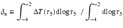 |
|
| |
|
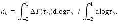 |
(37) |
 is the quantity
![\begin{displaymath}
\Delta T(\tau_5) \equiv [T(\tau_5) - T'(\tau_5)]/T_{\rm eff}
\end{displaymath}](/articles/aa/full/2008/30/aa09724-08/img228.gif) |
(38) |
where  is the temperature structure measured at the continuum optical depth at 5000 Å and
 the
corresponding quantity for a modified model atmosphere with the same fundamental parameters, but for which
line opacity sources have been neglected individually or simultaneously (such that the corresponding model is
unblanketed). The reason why
the
corresponding quantity for a modified model atmosphere with the same fundamental parameters, but for which
line opacity sources have been neglected individually or simultaneously (such that the corresponding model is
unblanketed). The reason why  and not
were chosen here is that the Rosseland mean is
directly affected by the spectral lines, in particular for the cooler stars, while we here wish to
separate these effects on the temperature structure from those on the
and not
were chosen here is that the Rosseland mean is
directly affected by the spectral lines, in particular for the cooler stars, while we here wish to
separate these effects on the temperature structure from those on the  scale.
We see from Fig. 5 that for a sequence of main-sequence models with solar metallicity the total blanketing
effect, both at the surface and in the deeper layers, is rather temperature independent. The structural effects of spectral lines
are surprisingly similar
for all solar-type stars. Thus, the mean surface cooling
amounts to about  of
and the mean heating of the layers below
of
and the mean heating of the layers below
 is about
  over most of the effective-temperature interval. I.e., the somewhat decreasing
importance of metal lines when proceeding towards the hot end of our effective-temperature interval is rather well compensated for
by the increasing hydrogen-line blanketing. The diminishing effects of metals for the cooler models are compensated for by
the molecular blanketing. These compensation effects explain why relatively old differential abundance analyses, made by
primitive model atmospheres such as scaled solar models, are often found to agree rather well with more recent results
based on models with much more complete atomic and molecular data.
over most of the effective-temperature interval. I.e., the somewhat decreasing
importance of metal lines when proceeding towards the hot end of our effective-temperature interval is rather well compensated for
by the increasing hydrogen-line blanketing. The diminishing effects of metals for the cooler models are compensated for by
the molecular blanketing. These compensation effects explain why relatively old differential abundance analyses, made by
primitive model atmospheres such as scaled solar models, are often found to agree rather well with more recent results
based on models with much more complete atomic and molecular data.
 |
Figure 6:
Similar to Fig. 5.
The structural effects of molecular lines separated for different species to show the
results of removing the line opacity of TiO, water, and CO, respectively. |
| Open with DEXTER |
In Fig. 6, we display the corresponding effects when
absorption by different molecular species is left out. It is seen that the only significant molecular effects at the surface
for these models are the surface cooling due to CO for moderately cool models and to H2O for the coolest ones and the surface heating due
to TiO, while in the deeper layers the significant back-warming is due to TiO
and H2O. Other molecules, like CN, play only
a very minor role in this respect.
 |
Figure 7:
The effects of dredge-up of CN-cycled material to the surfaces of
Pop I giant stars as illustrated by model atmospheres with different C and
N abundances.
In the top panel, carbon has been converted to nitrogen such that
the C/N abundance ratio has been lowered from the solar ratio
of 4.07 to 1.5, typical for the first dredge-up in low-mass stars. In
the lower panel, the ratio has been further lowered to 0.5
and there also the effects of changing the 12C/13C
ratio are displayed.
The stronger back-warming of the 3000 K models is due to the increased
importance of water as more oxygen gets available when the CO abundance is decreased by the reduction of carbon while the
heating effect at the surface merely reflects the inadequacy of
for this heavy line-blocked model - for
a plot of the temperature vs.
,
an increased cooling at the surface appears.
In the 5000 K model, the decreased CO cooling leads to a hotter surface. |
| Open with DEXTER |
The variation of certain abundances in the MARCS grid lead to effects on the models.
Such effects were explored for the CNO abundances of G and K giant models by Gustafsson et al. (1975), for M and S stars by
Plez et al. (2003) and for carbon stars by Lambert et al. (1986) and
Jørgensen et al. (1992). The results given here are
illustrative and complementary to those of previous studies - more detailed discussion of abundance effects will be presented
in later papers in this series.
The recent considerable downward corrections of solar CNO abundances by Asplund and collaborators (Grevesse et al. 2007, and references therein) are found to lead to very minor effects for most regions in the
parameter space spanned by the present grid. Thus, for the temperatures at
given
,
the effects are less
than
 for all depths and luminosities for giants at solar metallicity. The most pronounced effects in
the surface layers appear in models with
for all depths and luminosities for giants at solar metallicity. The most pronounced effects in
the surface layers appear in models with
 K and models with
 K
where the reduced
cooling due to H2O and CO, respectively, is visible.
K
where the reduced
cooling due to H2O and CO, respectively, is visible.
The CNO abundances in stars are modified through the first dredge-up along
the subgiant-giant branch, mostly converting C to N (see, e.g., Boothroyd & Sackmann 1999; Charbonnel 1994).
The effects of this on the model atmospheres
are, however, small or moderate, as illustrated in Fig. 7.
The two most important effects are again the
enhanced H2O surface cooling for the coolest models (since more O is available if C and thus CO is depleted), and a diminished
CO cooling for the somewhat hotter models. The changes due to effects by CN are marginal.
The accompanying changes of
 ratios
are obviously only of minor significance.
ratios
are obviously only of minor significance.
 |
Figure 8:
A sequence of MARCS spherical model atmospheres with
 K, log g = 0.0, K, log g = 0.0,
 .
The models have different abundance ratios, C/O, marked in the figure, but otherwise solar metal abundances.
Points on the temperature-pressure relations with log
.
The models have different abundance ratios, C/O, marked in the figure, but otherwise solar metal abundances.
Points on the temperature-pressure relations with log
 ,
-4, -3,-2, -1, 1, and 2 are marked with circles, which are filled for the carbon-rich models ( ,
-4, -3,-2, -1, 1, and 2 are marked with circles, which are filled for the carbon-rich models (
 ).
Points where log ).
Points where log
 are marked with
  .
The figure demonstrates the strongly increasing pressures at given temperature and optical depth as the C/O ratio increases, until C/O reaches 1.0 when the situation is drastically reversed as the opacities increase
and the pressures decrease again.
The models with .
The figure demonstrates the strongly increasing pressures at given temperature and optical depth as the C/O ratio increases, until C/O reaches 1.0 when the situation is drastically reversed as the opacities increase
and the pressures decrease again.
The models with
 show M-type model spectra,
those in the interval
show M-type model spectra,
those in the interval
 S-type spectra, while those with greater C/O show N-star spectra.
 |
| Open with DEXTER |
 |
Figure 9:
The effects of non-solar CNO abundance ratios on extreme Pop II star
models with
 K, log g=1.0,
[Me/H] = -3.0.
In the top panel, the carbon and nitrogen abundances have been
increased by factors of 10, 100, and 300 above the solar ratio
to iron, oxygen and all other elements. The heating in the
middle layers, primarily due to C2, is strong, and even more so
at depth, which is due to the increased electron pressures and
continuous opacities.
In the lower panel, oxygen is also enhanced.
The increased electron pressures in the more CN(O)-rich models
lowers the density and
convection efficiency at a certain optical depth which
increases the temperature gradient.
The major surface cooling agent in the outer surface layers is CO. K, log g=1.0,
[Me/H] = -3.0.
In the top panel, the carbon and nitrogen abundances have been
increased by factors of 10, 100, and 300 above the solar ratio
to iron, oxygen and all other elements. The heating in the
middle layers, primarily due to C2, is strong, and even more so
at depth, which is due to the increased electron pressures and
continuous opacities.
In the lower panel, oxygen is also enhanced.
The increased electron pressures in the more CN(O)-rich models
lowers the density and
convection efficiency at a certain optical depth which
increases the temperature gradient.
The major surface cooling agent in the outer surface layers is CO. |
| Open with DEXTER |
The most severe atmospheric effects of CNO abundance changes occur, however, when the carbon abundance is raised by dredge-up
on the asymptotic-giant branch and, as the carbon abundance approaches or exceeds that of oxygen, the star becomes an S or a C star, respectively,
with drastic changes in radiation fields and thus temperature-pressure structure.
This transition has been explored using MARCS models
(for references, see above), and will be further discussed in
Papers V and VI in the current series. As an illustration
here, however,
we present a sequence of models, with C/O ratios ranging from 0.5 to 2.4 in Fig. 8.
The most metal-poor stars known until now show severe departures from
``standard'' CNO abundances:
they seem to be comparatively very rich in CNO elements (cf., Christlieb et al. 2004; Frebel et al. 2005;
Norris et al. 2007, and references therein).
In general, there is a group of low-metallicity
stars with considerably enriched carbon abundances, so-called carbon-enriched metal-poor (CEMP) stars, (see, e.g., Aoki et al. 2007), which
may show carbon enrichments ranging in the interval between a factor of 10 and
1000 relative to a solar C/Fe, as well as
similarly considerable N enrichments and possibly also O enrichments.
The effects on the atmospheric structures from these enrichments are illustrated in Fig. 9 for one representative
CEMP giant model.
It is seen that the enhanced C and N abundances heat the layers
 considerably for these model parameters (a result which was also found
by Hill et al. 2000). Also, the deep layers get warmer, which is due to the increased electron contributions
from the enhanced carbon. This increases the H- opacity, which lowers the density at a given optical
depth and therefore reduces the convective energy flux, which increases the inner temperature gradient.
These effects change if O is also enhanced correspondingly. Then the CO cooling takes over in the surface layers,
and much of the C2 and CN heating absorption vanishes since most of the carbon is bound in the CO molecules.
considerably for these model parameters (a result which was also found
by Hill et al. 2000). Also, the deep layers get warmer, which is due to the increased electron contributions
from the enhanced carbon. This increases the H- opacity, which lowers the density at a given optical
depth and therefore reduces the convective energy flux, which increases the inner temperature gradient.
These effects change if O is also enhanced correspondingly. Then the CO cooling takes over in the surface layers,
and much of the C2 and CN heating absorption vanishes since most of the carbon is bound in the CO molecules.
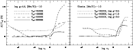 |
Figure 10:
The effects of an increase in the -element abundances by
+0.4 dex on the temperature structure of models of dwarfs and giants with [Fe/H] = -1.0.
The comparison model in each case is a corresponding model with no -element enhancement ([/Fe] = 0.0).
The increased electron pressure lowers the density and
convection efficiency at a certain Rosseland optical depth, which
increases the temperature gradient in the deeper parts of a model. |
| Open with DEXTER |
The effects of the observed increase of Fe] for galactic, though seemingly not all, metal-poor stars can also
be explored using the grid models. Although these changes are easily seen in spectra of the models, e.g., in the strengths of the
Mg and Ca lines, the effects on the temperature-pressure structures are only minor. As is seen in Fig. 10, they are, however, of
some significance for models with
 where the higher
Ti abundance increases the surface heating
as well as the back-warming of the TiO absorption. Simultaneously, the electron contributions from Mg and Ca
increase and raise the H- opacity, which partly reduces the effects of the
Ti abundance change.
As discussed above for the CEMP star models, the higher electron pressures also reduce the densities at a given optical depth, which
diminishes the convective flux and thus admits a stronger temperature gradient in the deep atmosphere.
where the higher
Ti abundance increases the surface heating
as well as the back-warming of the TiO absorption. Simultaneously, the electron contributions from Mg and Ca
increase and raise the H- opacity, which partly reduces the effects of the
Ti abundance change.
As discussed above for the CEMP star models, the higher electron pressures also reduce the densities at a given optical depth, which
diminishes the convective flux and thus admits a stronger temperature gradient in the deep atmosphere.
It should finally be noted that systematic errors in the models, due to missing opacities, departures from LTE
or convectively generated inhomogeneities and errors in calculated convective fluxes, may well vary systematically
with chemical composition. Thus, the trends discussed in the present section may have to be revised when more realistic
models are available.
In the present grid, there are models calculated with different microturbulence parameters
,
but with otherwise
identical input data. This makes it possible to systematically explore the dependence of the blanketing effects
on microturbulence. Before discussing the results, we will present some considerations of what one could expect.
An increased microturbulence enhances the blocking of the spectrum by isolated
saturated spectral lines, in proportion to
.
So, if all lines were saturated, one might estimate from
Eq. (35) that the back-warming
 would increase by about
 .
However, this is an upper limit since a
considerable fraction of the spectral lines (though not necessarily those that contribute most significantly
to the blocking) will not be saturated - their equivalent widths will be unaffected by a changing
and thus the total blocking
is not changed. Also, for more metal-rich stars the overlapping of strong lines reduces the differential
effects of a
increase as does the fact that many of these lines have strong damping wings. We thus
expect the effects of microturbulence changes on the back-warming to be small for the most metal-poor stars where
even the strongest lines are unsaturated,
then increase but finally level off for the most metal-rich and coolest models, and never reach the
estimated upper limit. These expectations are verified by the models, as is
illustrated in Fig. 11. The differential back-warming caused by an increased microturbulence parameter,
e.g., by a factor of 2, is of about the same magnitude as the result of doubling the metallicity. This suggests that the total blocking
contribution of lines on the flat part of the curve-of-growth (mainly sensitive
to
)
is of similar significance
as that of weak spectral lines (proportional in strength to the metallicity); this picture is complicated
by both the effects of lines on the damping-part of the curve-of-growth (with only a square-root dependence on abundance)
and the strong abundance sensitivity of some diatomic molecules.
.
However, this is an upper limit since a
considerable fraction of the spectral lines (though not necessarily those that contribute most significantly
to the blocking) will not be saturated - their equivalent widths will be unaffected by a changing
and thus the total blocking
is not changed. Also, for more metal-rich stars the overlapping of strong lines reduces the differential
effects of a
increase as does the fact that many of these lines have strong damping wings. We thus
expect the effects of microturbulence changes on the back-warming to be small for the most metal-poor stars where
even the strongest lines are unsaturated,
then increase but finally level off for the most metal-rich and coolest models, and never reach the
estimated upper limit. These expectations are verified by the models, as is
illustrated in Fig. 11. The differential back-warming caused by an increased microturbulence parameter,
e.g., by a factor of 2, is of about the same magnitude as the result of doubling the metallicity. This suggests that the total blocking
contribution of lines on the flat part of the curve-of-growth (mainly sensitive
to
)
is of similar significance
as that of weak spectral lines (proportional in strength to the metallicity); this picture is complicated
by both the effects of lines on the damping-part of the curve-of-growth (with only a square-root dependence on abundance)
and the strong abundance sensitivity of some diatomic molecules.
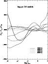 |
Figure 11:
for models with different microturbulence parameters
,
minus
for a model with
 km s-1, for solar
composition, log g=2.0 and different effective temperatures. Thick lines denote models with km s-1, for solar
composition, log g=2.0 and different effective temperatures. Thick lines denote models with
 km s-1, thin lines with km s-1, thin lines with
 km s-1. km s-1. |
| Open with DEXTER |
With regard to the differential
blanketing effects in the upper atmosphere when the microturbulence parameter is changed, the situation is not quite
obvious. The first, heating, part of the radiation equilibrium
integral in Eq. (30) will not change in itself if only the line-absorption
profiles become broader. If the effects
on
are taken into consideration, the decrease of the intensity over larger wavelength regions by the widening of the lines will,
as long as they are weak, be compensated for by the increase of
in the line centre.
However, for saturated lines,
will be reduced over broader wavelength intervals
when
is increased, and thus the heating term will become smaller. The second, cooling, term
will not change from a broadening of the
line profiles. Thus, a net cooling is expected to occur. We see from Fig. 11 that, in practice,
increasing
from 1 to 2 km s-1 leads to some moderate cooling (on the order of  in
in
 )
of the upper layers for all effective
temperatures, while further increase up to 10 km s-1 leads to further cooling
(by up to
)
of the upper layers for all effective
temperatures, while further increase up to 10 km s-1 leads to further cooling
(by up to  ,
for the coolest models), however,
this balance shifts to heating in the very surface layers.
,
for the coolest models), however,
this balance shifts to heating in the very surface layers.
Changes in the macroturbulent parameter (classically representing velocity shifts on geometrical
scales corresponding to at least one optical depth unit in the continuum) are not able to change the model structures through
radiative field changes. See Sect. 3 above concerning effects of changes in the turbulent pressure, which may be related to both macro- and
microturbulent motions.
Real stellar atmospheres are not believed to be well represented by the concepts of micro- and macroturbulence. Velocity
gradients on intermediate scales are of vital importance, as has been shown by convective
simulations (Nordlund & Dravins 1990; Asplund et al. 2000a), and global gradients caused by pulsations
as demonstrated in Lederer et al. (2006) and references therein. With respect to the effects on the radiative field, these gradients
allow for more heating in
spectral lines since the gas high up in the atmosphere may absorb hot radiation from lower layers that was not absorbed below;
similarly, the gas may cool more efficiently through spectral lines since the shifts make the gas more transparent in overlying
layers. However, even more important are the hydrodynamical effects due to gas expansion and compression
on the energy balance. Altogether, this makes the representation
of the energy balance in real stars by classical models quite problematic; also, there is no hope
to gain further insight into the physics of these systems by fine-tuning the turbulence parameters.
The properties of spherically-symmetric model atmospheres for late-type stars have been discussed or commented upon in
numerous studies. The area was first pioneered by Schmid-Burgk & Scholz (1975) and Schmid-Burgk et al. (1981, and papers cited therein);
and later explored by Plez (1990), Plez et al.
(1992); Jørgensen et al. (1992);
Hauschildt et al. (1999);
and Heiter & Eriksson (2006).
The papers by Plez and collaborators, by Jørgensen and collaborators, and by Heiter & Eriksson, all
build on earlier versions of the MARCS code. These papers demonstrate that the effects of sphericity are
in general important for the temperature structures, causing relative temperature effects on the order of 1% or more, for extensions of the atmosphere normalised on the stellar radius greater than about 2%.
The relative extensions scale roughly as g-1/2; the sphericity effects are thus
mainly important for low-gravity models.
These papers do not, however, systematically
explore the effects on the models and fluxes of changing from plane-parallel to spherical symmetric
geometry. Here, some further comments will be made on this topic on the basis of the new
model grid.
The extension z0 of the stellar atmosphere, measured as the geometrical thickness of the
atmosphere (for instance, defined as the layers with
 )
is a key
factor in the discussions.
It is easy to estimate the extension from the hydrostatic-equilibrium
equation, the definition of optical depth and the gas law for an ideal gas. The relative thickness of the
atmosphere from optical depth
up toward the surface at
)
is a key
factor in the discussions.
It is easy to estimate the extension from the hydrostatic-equilibrium
equation, the definition of optical depth and the gas law for an ideal gas. The relative thickness of the
atmosphere from optical depth
up toward the surface at  is thus:
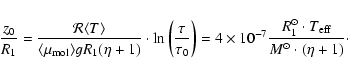 |
(39) |
Here, we have assumed the variation of the pressure in the atmosphere to be dominated by the density
variation - the temperature and the mean molecular weight
in the gas law were thus approximated by a
constant characteristic temperature and molecular weight,
 and
and
 (here set = 1.26), respectively.
The mass absorption coefficient (opacity per gram)
(here set = 1.26), respectively.
The mass absorption coefficient (opacity per gram)
 is assumed to vary (only) with the density ,
 .
The model radius and mass are
.
The model radius and mass are  and
and  ,
respectively, in solar units.
,
respectively, in solar units.
![\begin{figure}
\par\includegraphics[width=8.5cm,clip]{9724fg12.eps}
\end{figure}](/articles/aa/full/2008/30/aa09724-08/Timg262.gif) |
Figure 12:
The value of C as calculated from Eq. (40) with model values of z0/R1 for a set of models with
ranging from 3000 K to 8000 K (with bigger symbols the higher the effective temperature)
and metallicities [Me/H] = 0.0, except for two models with [Me/H] = -1.0, which are
attached with thin lines to corresponding [Me/H] = 0.0 models.  was
chosen = 1. The value of C when based on the value of the
extension z0/R1 estimated from Eq. (39) is 1.0 and shown by the horizontal dotted line.
was
chosen = 1. The value of C when based on the value of the
extension z0/R1 estimated from Eq. (39) is 1.0 and shown by the horizontal dotted line. |
| Open with DEXTER |
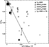 |
Figure 13:
The difference in the surface temperature (at log
)
between spherical and
plane-parallel models with
ranging from 3000 K to 7000 K (with bigger symbols the higher log g)
and metallicities [Me/H] = 0.0, except for two models with
![$\rm [Me/H]=-1.0$](/articles/aa/full/2008/30/aa09724-08/img34.gif) ,
which are
attached with thin lines to corresponding [Me/H] = 0.0 models
(the lower symbols in the pairs representing the more metal-poor
models). Three models at ,
which are
attached with thin lines to corresponding [Me/H] = 0.0 models
(the lower symbols in the pairs representing the more metal-poor
models). Three models at
 K have also been calculated with TiO absorption neglected and are denoted by
crosses - it is seen
that the positions of these models depart very significantly from the corresponding standard models. The relation
according to Eq. (41) is shown as a straight line. K have also been calculated with TiO absorption neglected and are denoted by
crosses - it is seen
that the positions of these models depart very significantly from the corresponding standard models. The relation
according to Eq. (41) is shown as a straight line. |
| Open with DEXTER |
According to our analytical estimate of the relative extension in Eq. (39),
the quantity
![\begin{displaymath}
C=2.5\times 10^6\left[{z_0\over R_1}\right]\cdot {M^\odot \over R_1^\odot \cdot T_{\rm eff} } \cdot(\eta+1)
\end{displaymath}](/articles/aa/full/2008/30/aa09724-08/img265.gif) |
(40) |
should be approximately constant and equal to 1.0. It is seen in Fig. 12 that the
relative extension is fairly well accounted for by the approximate expression, and that the choice
of  is a reasonable fit
for an extensive part of the HR diagram, which is to be expected since the dominating H- absorption per gram
is roughly proportional to the pressure. Note that the relative extension of an atmosphere
is relatively independent of the magnitude of the opacity, which cancels in the zero-order approximation. A
depth-variation of
is a reasonable fit
for an extensive part of the HR diagram, which is to be expected since the dominating H- absorption per gram
is roughly proportional to the pressure. Note that the relative extension of an atmosphere
is relatively independent of the magnitude of the opacity, which cancels in the zero-order approximation. A
depth-variation of  is of some significance, but only marginally so. The most
important sphericity effects related to the opacity are more indirect, through the effects that a changed temperature structure
may lead to, in particular when molecular absorption is switched on, as will be demonstrated below.
is of some significance, but only marginally so. The most
important sphericity effects related to the opacity are more indirect, through the effects that a changed temperature structure
may lead to, in particular when molecular absorption is switched on, as will be demonstrated below.
We now turn to the sphericity effects on the temperature structure of the models. The temperature in radiative
equilibrium is set by the radiative field, following Eq. (30). The basic effects due to sphericity at a
point high up in a stellar atmosphere come
from the general dilution of the radiative field, partially due to the
absence of incoming radiation from angles
 where
where  gradually increases the further from the
optically-thick layers that the point is situated. Basically, this leads to less radiative heating of the
upper layers of the atmosphere and thus leads to cooler temperatures there. One may prove that this reduction of the mean intensity
for small extensions will scale with
(z0/R1)1/2.
For larger distances from the star, a simple and approximative estimate for the temperature
effect, was presented by Gustafsson et al. (1975; see also Böhm-Vitense 1972) who assumed that the radiative
flux should be roughly proportional to radius r-2 and to temperature T4 as one may estimate from
Stefan-Boltzmann's law. This leads to the estimate
gradually increases the further from the
optically-thick layers that the point is situated. Basically, this leads to less radiative heating of the
upper layers of the atmosphere and thus leads to cooler temperatures there. One may prove that this reduction of the mean intensity
for small extensions will scale with
(z0/R1)1/2.
For larger distances from the star, a simple and approximative estimate for the temperature
effect, was presented by Gustafsson et al. (1975; see also Böhm-Vitense 1972) who assumed that the radiative
flux should be roughly proportional to radius r-2 and to temperature T4 as one may estimate from
Stefan-Boltzmann's law. This leads to the estimate
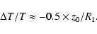 |
(41) |
The effects of sphericity on the temperature structures of the models are shown in Fig. 13
and compared with the approximate expression in Eq. (41). The agreement is satisfactory,
though certainly not perfect, which is
partially explained by the approximations made in deriving it. As important are the effects of
the wavelength dependence of
,
which gives the mean
intensity
and the
Planck function  in the radiation equilibrium integrals of Eq. (30) different weights for
different models, depending in particular on the molecular absorption and resulting in the large scatter
in Fig. 13.
in the radiation equilibrium integrals of Eq. (30) different weights for
different models, depending in particular on the molecular absorption and resulting in the large scatter
in Fig. 13.
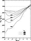 |
Figure 14:
The difference between temperature structures of spherically symmetric and corresponding plane-parallel models with
log g=1.0,
 ,
[Me/H] = 0.0, and
ranging from 3000 K to 6000 K. The complex variation of the sphericity effects in the upper layers
when TiO sets in as a heating agent at ,
[Me/H] = 0.0, and
ranging from 3000 K to 6000 K. The complex variation of the sphericity effects in the upper layers
when TiO sets in as a heating agent at
 K is illustrated. K is illustrated. |
| Open with DEXTER |
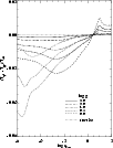 |
Figure 15:
The difference between temperature structures of spherically-symmetric and corresponding plane-parallel models with
K and
different log g.
and
[Me/H] = 0.0, and with the TiO absorption alternatively switched on and off (dashed lines, the gravities of these can be
traced via the models to which they adhere at depth). The complex variation of the sphericity effects in the upper layers
due to TiO is illustrated. |
| Open with DEXTER |
Now turning to the detailed model results, the sphericity effects on
are shown in Fig. 14 as a function of
for a sequence
of supergiant models with different effective temperatures. Obviously, the effects shift with
.
First being relatively small for the hottest models, they considerably increase for
 ,
then diminish again to reach a minimum at
about 3800 K and finally again increase strongly as
goes towards 3000 K. This behaviour may be interpreted as a coupling
between the sphericity effects and the effects of molecular blanketing.
The coupling may show up as positive or negative feedback. Sphericity cools the upper layers, relative to a plane-parallel model,
and the molecular formation increases. Around 5000 K this leads to a strong surface cooling by CO. For cooler models TiO forms, which
conversely heats the upper atmosphere. Finally, H2O takes over as a dominating opacity source, and that again cools the model surface. That
this explains the behaviour can be tested by blocking out different molecular opacities from the model calculations. In Fig. 15 we thus
show a sequence of models at
,
then diminish again to reach a minimum at
about 3800 K and finally again increase strongly as
goes towards 3000 K. This behaviour may be interpreted as a coupling
between the sphericity effects and the effects of molecular blanketing.
The coupling may show up as positive or negative feedback. Sphericity cools the upper layers, relative to a plane-parallel model,
and the molecular formation increases. Around 5000 K this leads to a strong surface cooling by CO. For cooler models TiO forms, which
conversely heats the upper atmosphere. Finally, H2O takes over as a dominating opacity source, and that again cools the model surface. That
this explains the behaviour can be tested by blocking out different molecular opacities from the model calculations. In Fig. 15 we thus
show a sequence of models at
 with different log g and with and without TiO. It is clear that the differential
sphericity effects above
are changed significantly by the TiO absorption. From this figure we also see that the sphericity effects
in the temperature structure are significantly greater than 1% for models with log
with different log g and with and without TiO. It is clear that the differential
sphericity effects above
are changed significantly by the TiO absorption. From this figure we also see that the sphericity effects
in the temperature structure are significantly greater than 1% for models with log  .
However, if turbulent pressures are taken
into account this latter value may be higher, according to Eq. (7).
.
However, if turbulent pressures are taken
into account this latter value may be higher, according to Eq. (7).
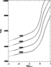 |
Figure 16:
MARCS model atmospheres (solid) for dwarf stars with log g=4.5, [Me/H] = 0.0 and corresponding models from the
Castelli & Kurucz ODFNEW grid (dashed). The curves are labelled with relevant values of
. |
| Open with DEXTER |
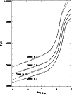 |
Figure 17:
MARCS model atmospheres for giants and supergiants with [Me/H] = 0.0 (solid) and corresponding models from the
recent Castelli & Kurucz grid (dashed). The curves are labelled with relevant values of
and log g. |
| Open with DEXTER |
We now compare MARCS grid models with the models of other existing grids, but confine this comparison to the temperature
structures. Some additional comments on calculated fluxes will be be made in
subsequent papers of this series.
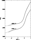 |
Figure 18:
MARCS model atmospheres with [Me/H] = -2.0 (solid) and corresponding models from the
Castelli & Kurucz ODFNEW grid (dashed). The curves are labelled with relevant values of
and log g. |
| Open with DEXTER |
The most extensive and widely-used grid of models for most of our parameter space are the plane-parallel models
of Kurucz and collaborators (available on
http://kurucz.harvard.edu). Among the different sets of models
published there, it is particularly relevant
to compare our models with those calculated by Castelli & Kurucz (2003)
with a standard mixing-length theory (without ``convective overshoot''), which also seem to produce
more consistent model parameters when applied to real data (Castelli et al. 1997).
Some sample comparisons of model structures are shown in Figs. 16-18. It is seen that the
agreement in the temperature structures is almost perfect for the models of solar-type dwarf stars of different
metallicities. This is also true for models of early M dwarfs. For the models of giants and supergiants, the
agreement is again good, although the MARCS models tend to be some 10-80 K cooler in the surface layers where
 .
The agreement is also very satisfactory if pressures or densities are intercompared.
In view of the fact that these two grids of models are made with two totally independent numerical methods and
computer codes, with independent choices of basic data (although Kurucz's extensive lists of atomic line transitions
are key data underlying both grids), this overall agreement is both satisfactory and gratifying.
.
The agreement is also very satisfactory if pressures or densities are intercompared.
In view of the fact that these two grids of models are made with two totally independent numerical methods and
computer codes, with independent choices of basic data (although Kurucz's extensive lists of atomic line transitions
are key data underlying both grids), this overall agreement is both satisfactory and gratifying.
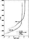 |
Figure 19:
Model atmospheres with solar abundances, from the MARCS, NextGen, and PHOENIX-ACES-2008 grids and (for
K) the
ODFNEW Castelli & Kurucz grid. The log g parameter is 3.0 (5000 K) and 0.0 (3000 K), respectively. The MARCS and NextGen models are
spherically symmetric with
 while the Kurucz model is plane-parallel. Along the MARCS curve
every decade in
is marked by a
while the Kurucz model is plane-parallel. Along the MARCS curve
every decade in
is marked by a  sign, and
 by a .
The general impression of a better agreement between MARCS and Castelli & Kurucz
models than between MARCS and NextGen models is also shown if the temperature is plotted
relative to optical depth.
by a .
The general impression of a better agreement between MARCS and Castelli & Kurucz
models than between MARCS and NextGen models is also shown if the temperature is plotted
relative to optical depth. |
| Open with DEXTER |
![\begin{figure}
\par\includegraphics[width=8.5cm,clip]{9724fg20.eps}
\end{figure}](/articles/aa/full/2008/30/aa09724-08/Timg285.gif) |
Figure 20:
Model atmospheres with solar abundances, from the present MARCS grid compared with corresponding MARCS models from
Bell et al. (1976, BGEN, dashed) and with one model from Plez (1992). The
log g parameter is 3.0 and the geometry is plane-parallel for the 6000 K, 5000 K and 4000 K models; the 3000 K models
are spherically symmetric with M=5  and log g=0.0.
 |
| Open with DEXTER |
The situation was somewhat less satisfactory for models from the NextGen grid of spherically-symmetric models, calculated with the
PHOENIX code (Hauschildt et al.
1999, models obtained by private communication in 1996). In the inner photospheres the agreement is good, but again a difference systematically appears at the surface,
starting around
 ,
with the MARCS models
being cooler, but now by as much as typically 250 K. (As is seen in Fig. 19, the agreement between the Castelli & Kurucz and
the MARCS models is generally much better than with the NextGen models.) However, more recent LTE models (PHOENIX-ACES-2008) obtained
by Hauschildt with an updated
version of the PHOENIX code (Hauschildt, private communication) and which are also based on Kurucz line data, agree very well with the MARCS models. The basic reason for this improvement in the fit seems to be due to changes in
molecular opacities. Again, the present overall fit is very satisfactory in view of the independence of the methods of the MARCS and PHOENIX
teams.
,
with the MARCS models
being cooler, but now by as much as typically 250 K. (As is seen in Fig. 19, the agreement between the Castelli & Kurucz and
the MARCS models is generally much better than with the NextGen models.) However, more recent LTE models (PHOENIX-ACES-2008) obtained
by Hauschildt with an updated
version of the PHOENIX code (Hauschildt, private communication) and which are also based on Kurucz line data, agree very well with the MARCS models. The basic reason for this improvement in the fit seems to be due to changes in
molecular opacities. Again, the present overall fit is very satisfactory in view of the independence of the methods of the MARCS and PHOENIX
teams.
A number of comparisons with models made by previous versions of MARCS have also been performed. In Fig. 20, we thus compare with
models of G and K giants (Bell et al. 1976) calculated with the first version of MARCS. It is seen that the present temperature structures agree
quite well with the older ones in spite of the
much more incomplete line absorption data of those models. (An exception from this is seen in the outer layers of the 4000 K model, where the
TiO absorption, missing in the BGEN models, contributes a surface heating of the more recent model).
The pressures in the present models are, however, significantly lower, which
reflects their more heavy opacities. The good agreement in the temperature structures must thus, at least partially, be
fortuitous, e.g., reflecting that the line absorption missing in the 1976 models
is not heavily biassed towards the ultraviolet or the red spectral regions relative to the absorption that is now included.
In Fig. 20, we also show
one example where a spherically-symmetric model for a late-type M supergiant is compared with a previous
spherically-symmetric MARCS model of Plez et al. (1992). The considerable
differences in the upper photosphere are due to the new and improved molecular data used now and its more detailed
representation, in particular, for the H2O absorption.
It is useful to be able to interpolate the model structures to
a set of parameters
,
 ,
and [Me/H] different
from those tabulated in the grid. Such an interpolation is not completely
straightforward, as strong non-linearities appear in the behaviour of some
of the thermodynamic variables when stellar parameters are varied.
One program was developed by Masseron (2006) and extensively tested
by him on a previous grid of MARCS models encompassing the following range of parameters:
3800
,
and [Me/H] different
from those tabulated in the grid. Such an interpolation is not completely
straightforward, as strong non-linearities appear in the behaviour of some
of the thermodynamic variables when stellar parameters are varied.
One program was developed by Masseron (2006) and extensively tested
by him on a previous grid of MARCS models encompassing the following range of parameters:
3800
 K,
K,
 ,
,
![$-4.0<{\rm [Me/H]}<0.0$](/articles/aa/full/2008/30/aa09724-08/img290.gif) .
It interpolates
.
It interpolates
 ,
and the geometrical depth
as a function of
.
The interpolated model must lie inside a complete cube of existing models
in the parameter space (
,
,
[Me/H]), and the interpolation
is optimized to account for non-linearities in the grid.
With the actual grid parameter steps, maximum errors in the interpolated quantities
should remain below 0.25% for T and a few % for
and ,
whereas
and the column density (rhox) are more difficult to interpolate.
The program, with a detailed user manual, is available on the MARCS web site:
http://marcs.astro.uu.se.
An interpolation routine, applied to structures, as well as fluxes and colours of models by
Kurucz and collaborators, has
also been described by Nendwich et al. (2004), see also
Valenti & Fischer (2005).
,
and the geometrical depth
as a function of
.
The interpolated model must lie inside a complete cube of existing models
in the parameter space (
,
,
[Me/H]), and the interpolation
is optimized to account for non-linearities in the grid.
With the actual grid parameter steps, maximum errors in the interpolated quantities
should remain below 0.25% for T and a few % for
and ,
whereas
and the column density (rhox) are more difficult to interpolate.
The program, with a detailed user manual, is available on the MARCS web site:
http://marcs.astro.uu.se.
An interpolation routine, applied to structures, as well as fluxes and colours of models by
Kurucz and collaborators, has
also been described by Nendwich et al. (2004), see also
Valenti & Fischer (2005).
It will certainly take additional time before model atmospheres for late-type stars are regularly
constructed with physically more adequate assumptions than the standard ones - of spherical symmetry,
mixing-length convection and LTE - adopted here. Until then, standard models will be the common
choice in, e.g., abundance analyses. Here we have presented such a grid of standard
models to the state of the art. It includes model atmospheres for stars of
spectral types from F to M, as well as carbon stars and Pop II stars of different metallicities.
The assumptions, physical data used and numerical methods have been described, and a number of general properties
of the models have been illustrated. In particular, we have discussed the effects of blanketing and sphericity
in some detail and tested several of the existing approximate analytical estimates of these effects
and found them to work quite well. Also, already existing grids, such as the
grid of plane-parallel models by Castelli & Kurucz and the new PHOENIX grid, have been compared with and the
agreement has been found to be excellent in the region of overlapping parameters. This is particularly
gratifying in view of the fact that the different approaches, as regards numerical methods and codes and
to a considerable degree also the selection of data, are independent. We may then basically view the
calculation of standard 1D LTE model atmospheres as routine, but important improvements in line absorption
data are still needed and certainly not easily achieved. This is also true for data for dust formation and
dust opacities.
Further presentations and discussions of particular properties of these
models will appear in subsequent papers in this series. Hopefully, these will also serve as starting
points for further studies of the adequacy and shortcomings of the standard models, and as a stimulus
for endeavours to set higher standards in the art of modelling stellar atmospheres in the future.
Acknowledgements
We thank the Swedish Science Research Council and the Centre National de la Recherche Scientifique for long-standing support during the
years. B.P. thanks Sveneric Johansson for his hospitality for several years at the Department for Physics at Lund.
Previous
collaborators in the development of the MARCS code are also thanked: Roger A Bell, Martin Asplund,
John Brett, Leen Decin, Ulf Ekberg, Göran Hammarbäck, Dan Kiselman, Michelle Mizuno-Wiedner, Olle Morell, Nils Olander, Mikael Saxner
and Nicole van der Bliek, as well as contributors and critics
of important atomic and molecular data: Jan Almlöf, Bernhard Aringer, Paul Barklem, Manuel Bautista, Aleksandra Borysow, Alan Irwin,
Per Jensen, Sveneric Johansson, Alain Jorissen, Bob Kurucz, David Lambert, Mats Larsson,
Bo Lindgren, Nik Piskunov, Francois and Monique Querci, Jaques Sauval, Per Siegbahn and Georg Ole Sørensen. Peter Hauschildt is thanked
for providing PHOENIX models for comparison and Thomas Masseron for providing his interpolation routine for MARCS models.
Martin Asplund, Ulrike Heiter, Bob Kurucz, Jeff Linsky and Amy Mednick are thanked for valuable comments on the manuscript.
- Alvarez, R., &
Plez, B. 1998, A&A, 330, 1109 [NASA ADS]
(In the text)
- Alvarez, R.,
Lancon, A., Plez, B., et al. 2000, A&A, 353, 322 [NASA ADS]
(In the text)
- Anderson, L. S.
1989, ApJ, 339, 558 [NASA ADS] [CrossRef]
(In the text)
- Anstee, S. D., &
O'Mara, B. J. 1995, MNRAS, 276, 859 [NASA ADS]
(In the text)
- Aoki, W., Beers, T. C.,
Christlieb, N., et al. 2007, ApJ, 665, 492 [NASA ADS] [CrossRef]
(In the text)
- Asplund, M.,
Gustafsson, B., Kiselman, D., & Eriksson, K. 1997, A&A,
323, 286 [NASA ADS]
(In the text)
- Asplund, M.,
Nordlund, Å., Trampedach, R., & Stein, R. F. 1999,
A&A, 346, L17 [NASA ADS]
(In the text)
- Asplund, M.,
Nordlund, Å., Trampedach, R., Allende Prieto, C., & Stein,
R. F. 2000a, A&A, 359, 729 [NASA ADS]
(In the text)
- Asplund, M.,
Gustafsson, B., Lambert, D. L., & Rao, N. K. 2000b, A&A,
353, 287 [NASA ADS]
- Auer, L. H., &
Mihalas, D. 1970, MNRAS, 149, 65 [NASA ADS]
(In the text)
- Barber, R. J.,
Tennyson, J., Harris, G. J., & Tolchenov, R. N. 2006, MNRAS,
368, 1087 [NASA ADS] [CrossRef]
- Barklem, P., &
Aspelund-Johansson, J. 2005, A&A, 435, 373 [NASA ADS] [CrossRef] [EDP Sciences]
(In the text)
- Barklem, P.,
Piskunov, N., & O'Mara, B. J. 2000a, A&AS, 142, 467 [NASA ADS] [CrossRef] [EDP Sciences]
(In the text)
- Barklem, P.,
Piskunov, N., & O'Mara, B. J. 2000b, A&A, 363, 1091 [NASA ADS]
- Barklem, P., &
Piskunov, N. 2003, IAU Symp., 210, E28
(In the text)
- Bautista, M. A.
1997, A&AS, 122, 167 [NASA ADS] [CrossRef] [EDP Sciences]
(In the text)
- Bell, K. L., &
Berrington, K. A. 1987, J. Phys. B, 20, 801 [NASA ADS] [CrossRef]
- Bell, K. L., Hibbert, K.
A., & Berrington, K. A. 1988, J. Phys. B, 21, 2319 [NASA ADS] [CrossRef]
- Bell, R. A. 1971, MNRAS,
154, 343 [NASA ADS]
(In the text)
- Bell, R. A., &
Gustafsson, B. 1989, MNRAS, 236, 653 [NASA ADS]
(In the text)
- Bell, R. A., Eriksson,
K., Gustafsson, B., & Nordlund, Å. 1976, A&AS, 23,
37 [NASA ADS]
(In the text)
- Bensby, T.,
Feltzing, S., Lundström, I., & Ilyiin, I. 2005, A&A,
433, 185 [NASA ADS] [CrossRef] [EDP Sciences]
(In the text)
- Bessell, M. S.,
Castelli, F., & Plez, B. 1998, A&A, 333, 231 [NASA ADS]; A&A, 337,
321
(In the text)
- Blackwell, D.
E., Booth, A. J., Petford, A. D., et al. 1989, MNRAS, 236, 235 [NASA ADS]
(In the text)
- Böhm-Vitense, E. 1972, A&A, 17,
335 [NASA ADS]
(In the text)
- Boothroyd, A.
I., & Sackmann, I.-J. 1999, ApJ, 510, 232 [NASA ADS] [CrossRef]
(In the text)
- Borysow, A.,
Jørgensen, U. G., & Fu, Y. 2001, JQRST, 68, 235
- Bowen, G. 1988, ApJ,
329, 299 [NASA ADS] [CrossRef]
(In the text)
- Brault, J., &
Neckel, H. 1987, Spectral Atlas of Solar Disk-averaged and
Disk-center Intensity from 3290 to 12 510 Å, unpublished
(electronic copy by anonymous ftp from ftp.hs.uni-hamburg.de;
Directory /pub/outgoing/fts-atlas)
(In the text)
- Brett, J. M., &
Plez, B. 1993, PASAu, 10, 250 [NASA ADS]
(In the text)
- Bues, I., & Wehrse,
R. 1976, A&A, 51, 461 [NASA ADS]
- Carbon, D. F. 1979,
ARA&A, 17, 513 [NASA ADS] [CrossRef]
(In the text)
- Carbon, D. F., &
Gingerich, O. 1969, Proc. 3rd Harvard-Smithsonian Conf. on Stellar
Atmospheres, ed. O. Gingerich, Cambridge, Massachusettes Inst. of
Technology, 377
(In the text)
- Castelli, F.,
& Kurucz, R. L. 2003, IAU Symp., 210, A20
[arXiv:astro-ph/0405087]
(In the text)
- Castelli, F.,
Gratton, R. G., & Kurucz, R. L. 1997, A&A, 318, 841 [NASA ADS];
A&A, 324, 432
(In the text)
- Cayrel, R., Depagne,
E., Spite, M., et al. 2004, A&A, 416, 1117 [NASA ADS] [CrossRef] [EDP Sciences]
(In the text)
- Charbonnel,
C. 1994, A&A, 282, 811 [NASA ADS]
(In the text)
- Christlieb,
N., Gustafsson, B., Korn, A. J., et al. 2004, ApJ, 603, 708 [NASA ADS] [CrossRef]
(In the text)
- Dalgarno, A.,
& Williams, D. A. 1962, ApJ, 136, 690 [NASA ADS] [CrossRef]
- Däppen, W.,
Anderson, L., & Mihalas, D. 1987, ApJ, 319, 195 [NASA ADS] [CrossRef]
(In the text)
- Decin, L., Waelkens,
C., Eriksson, K., et al. 2000, A&A, 364, 137 [NASA ADS]
(In the text)
- Decin, L.,
Vanderbussche, B., Waelkens, C., et al. 2003, A&A, 400,
709 [NASA ADS] [CrossRef] [EDP Sciences]
(In the text)
- Doyle, R. O. 1968,
ApJ, 153, 987 [NASA ADS] [CrossRef]
- Edvardsson,
B., Andersen., J., Gustafsson, B., et al. 1993, A&A, 275,
101 [NASA ADS]
(In the text)
- Edvardsson,
B., Eriksson, K., Gustafsson, B., et al. 2008, A&A, to be
submitted
- Ekberg, U.,
Eriksson, K., & Gustafsson, B. 1986, A&A, 167, 304 [NASA ADS]
(In the text)
- Feautrier, P.
1964, C.R. Acad. Sci. 258, 3189 [NASA ADS]
(In the text)
- Fleischer, A.
J., Gauger, A., & Sedlmayr, E. 1992, A&A, 266, 321 [NASA ADS]
(In the text)
- Fluks, M. A., Plez,
B., The, P. S., et al. 1994, A&AS, 105, 311 [NASA ADS]
(In the text)
- Frebel, A., Aoki,
W., Christlieb, N., et al. 2005, Nature, 434, 871 [NASA ADS] [CrossRef]
(In the text)
- Freytag, B. 2001,
in 11th Cambridge Workshop on Cool Stars, Stellar Systems and the
Sun (ASP: San Francisco), 785
(In the text)
- Fuhrmann, K.
1998, A&A, 338, 161 [NASA ADS]
(In the text)
- Gibson, G. E., &
Heitler, W. 1928, Z. Phys., 49, 465 [NASA ADS] [CrossRef]
(In the text)
- Gillis, J. R.,
Goldman, A., Stark, G., et al. 2001, JQSRT, 68, 225 [NASA ADS]
(In the text)
- Gingerich, O.
1964, SAO Spec. Rep., 167 [NASA ADS]
- Goldman, A.,
Schoenfeld, W. G., Goorvitch, D., et al. 1998, JQSRT, 59, 453 [NASA ADS]
- Goorvitch, D.
1994, ApJS, 95, 535 [NASA ADS] [CrossRef]
- Grevesse, N.,
& Sauval, A. J. 1998, Space Science Rev., 85, 161 [NASA ADS] [CrossRef]
(In the text)
- Grevesse, N.,
Asplund, M., & Sauval, A. J. 2007, Space Sci. Rev., 130,
105 [NASA ADS] [CrossRef]
(In the text)
- Gustafsson,
B., & Bell, R. A. 1979, A&A, 74, 313 [NASA ADS]
(In the text)
- Gustafsson,
B., & Jørgensen, U. G. 1994, A&AR, 6, 19 [NASA ADS]
(In the text)
- Gustafsson,
B., & Nissen, P. E. 1972, A&A, 19, 261 [NASA ADS]
(In the text)
- Gustafsson, B., & Olander, N. 1979,
Phys. Scr., 20, 570 [NASA ADS] [CrossRef]
- Gustafsson,
B., & Plez, B. 1992, Proc. International Coll., ed. C. de
Jager, & H. Nieuwenhuijzen (Amsterdam: North Holland), 86
(In the text)
- Gustafsson,
B., Bell, R. A., Eriksson, K., & Nordlund, Å. 1975,
A&A, 42, 407 [NASA ADS]
(In the text)
- Gustafsson,
M., & Frommhold, L. 2001, ApJ, 546, 1168 [NASA ADS] [CrossRef]
- Gustafsson,
M., & Frommhold, L. 2003, A&A, 400, 1161 [NASA ADS] [CrossRef] [EDP Sciences]
- Harris, G. J.,
Polyansky, O., & Tennyson, J. 2002, ApJ, 578, 657 [NASA ADS] [CrossRef]
- Hartman, H.,
Derkatch, A., Donnelly, M. P., et al. 2003, A&A, 397, 1143 [NASA ADS] [CrossRef] [EDP Sciences]
(In the text)
- Hauschildt,
P. H., Allard, F., Ferguson, J., et al. 1999, ApJ, 525, 871 [NASA ADS] [CrossRef]
(In the text)
- Hauschildt,
P. H., Allard, F., Barman, T., et al. 2002, in Galactic Structure,
Stars and the Interstellar Medium, ed. C. Woodward, M. Bicay, &
J. Shull (ASP: San Francisco), 427
(In the text)
- Heiter, U., &
Eriksson, K. 2006, A&A, 452, 1039 [NASA ADS] [CrossRef] [EDP Sciences]
(In the text)
- Henyey, L., Vardya,
M. S., & Bodenheimer, P. 1965, ApJ, 142, 841 [NASA ADS] [CrossRef]
(In the text)
- Hill, V., Barbuy, B.,
Spite, M., et al. 2000, A&A, 353, 557 [NASA ADS]
(In the text)
- Holweger, H.,
& Müller, E. A. 1974, Sol. Phys., 39, 19 [NASA ADS] [CrossRef]
(In the text)
- Höfner, S.
1999, A&A, 346, L9 [NASA ADS]
(In the text)
- Höfner, S.,
& Dorfi, E. A. 1997, A&A, 319, 648 [NASA ADS]
(In the text)
- Höfner, S.,
Gautschy-Loidl, R., Aringer, B., & Jørgensen, U. G. 2003,
A&A, 399, 589 [NASA ADS] [CrossRef] [EDP Sciences]
(In the text)
- Irwin, A. W. 1981,
ApJS, 45, 621 [NASA ADS] [CrossRef]
(In the text)
- Irwin, A. W. 1988,
A&AS, 74, 145 [NASA ADS]
(In the text)
- John, T. L. 1975a,
MNRAS, 170, 5 [NASA ADS]
- John, T. L. 1975b,
MNRAS, 172, 305 [NASA ADS]
- John, T. L. 1994, MNRAS,
269, 871 [NASA ADS]
- John, T. L., &
Williams, R. J. 1975, MNRAS, 171, 7 [NASA ADS]
- Johnson, H. R.
1973, ApJ, 180, 81 [NASA ADS] [CrossRef]
(In the text)
- Johnson, H. R.,
Bernat, A. P., & Krupp, B. M. 1980, ApJS, 42, 501 [NASA ADS] [CrossRef]
(In the text)
- Jørgensen, U. G. 1989, ApJ, 344,
901 [NASA ADS] [CrossRef]
(In the text)
- Jørgensen, U. G. 1990, A&A, 232,
420 [NASA ADS]
(In the text)
- Jørgensen, U. G. 1994a, A&A, 284,
179 [NASA ADS]
(In the text)
- Jørgensen, U. G. 1994b, Proc. IAU
Coll., 146 [NASA ADS], ed. U. G. Jørgensen (New-York, Berlin, Heidelberg:
Springer-Verlag), 29
- Jørgensen, U. G. 1997, IAU Symp., 178,
441 [NASA ADS]
(In the text)
- Jørgensen, U. G. 2005, ASPC, 336,
269 [NASA ADS]
(In the text)
- Jørgensen, U. G., & Larsson, M.
1990, A&A, 238, 424 [NASA ADS]
- Jørgensen, U. G., & Johnson, H. R.
1992, A&A, 265, 168 [NASA ADS]
(In the text)
- Jørgensen, U. G., Almlöf, J.,
Gustafsson, B., et al. 1985, J. Chem. Phys., 83, 3034 [NASA ADS] [CrossRef]
(In the text)
- Jørgensen, U. G., Almlöf, J.,
& Siegbahn, P. E. M. 1989, ApJ, 343, 554 [NASA ADS] [CrossRef]
- Jørgensen, U. G., Johnson, H. R.,
& Nordlund, Å. 1992, A&A, 261, 263 [NASA ADS]
- Jørgensen, U. G., Larsson, M., Iwamae,
A., & Yu, B. 1996, A&A, 315, 204 [NASA ADS]
- Jørgensen, U. G., Hammer, D., Borysow,
A., et al. 2000, A&A, 361, 283 [NASA ADS]
- Jørgensen, U. G., Jensen, P.,
Sørensen, G. O., & Aringer, B. 2001, A&A, 372,
249 [NASA ADS] [CrossRef] [EDP Sciences]
(In the text)
- Karzas, W. J., &
Latter, R. 1961, ApJS, 6, 167 [NASA ADS] [CrossRef]
- Krupp, B. M., Collins,
J. G., & Johnson, H. R. 1978, ApJ, 219, 963 [NASA ADS] [CrossRef]
(In the text)
- Kurucz, R. L. 1979,
ApJS, 40, 1 [NASA ADS] [CrossRef]
(In the text)
- Kurucz, R. L. 1995a,
Kurucz CD-ROM, 15, Cambridge, Mass.: Smithsonian Astrophysical
Observatory
(In the text)
- Kurucz, R. L.
1995b, Laboratory and Astronomical High Resolution Spectra, ed. A.
J. Sauval, R. Blomme, & N. Grevesse, ASP Conf. Ser., 81,
583
- Kurucz, R. L.,
& Bell, B. 1995, Kurucz CD-ROM No. 23 [NASA ADS] [CrossRef], Cambridge, Mass:
Smithsonian, Astrophysical Observatory
- Kurucz, R. L., van
Dishoeck, E. F., & Tarafdar, S. P. 1987, ApJ, 322, 992 [NASA ADS] [CrossRef]
- Lambert, D. L.,
Gustafsson, B., Eriksson, K., & Hinkle, K. H. 1986, ApJS, 62,
373 [NASA ADS] [CrossRef]
(In the text)
- Langhoff, S. R.,
& Bauschlicher, C. W., Jr. 1993, Chem. Phys. Lett., 211,
305 [NASA ADS] [CrossRef]
- Lawler, J. E.,
Hartog, E. A. D., Labby, Z. E., et al. 2007, ApJS, 169, 120 [NASA ADS] [CrossRef]
(In the text)
- Lederer, M. T.,
Lebzelter, T., Aringer, B., et al. 2006, Mem. S.A.It, 77, 1008 [NASA ADS]
(In the text)
- Loidl, R., Lancon, A.,
& Jørgensen, U. G. 2001, A&A, 371, 1065 [NASA ADS] [CrossRef] [EDP Sciences]
(In the text)
- Masseron, T.
2006, Ph.D. Thesis, Obs. de Paris
(In the text)
- Massey, P., Plez,
B., Levesque, E. M., et al. 2007, [arXiv:0708.2847]
(In the text)
- Mihalas, D. 1964,
ApJS, 9, 321 [NASA ADS] [CrossRef]
- Mihalas, D. 1978,
Stellar Atmospheres, 2n [NASA ADS]d edn. (W. H. Freeman and Co., San
Francisco)
(In the text)
- Nave, G., Johansson, S.,
Learner, R. C. M., et al. 1994, ApJS, 94, 221 [NASA ADS] [CrossRef]
(In the text)
- Nendwich, J.,
Heiter, U., Kupka, F., et al. 2004, Comm. Astroseismol., 144,
43
(In the text)
- Nissen, P. E., Chen,
Y. Q., Asplund, M., et al. 2004, A&A, 415, 993 [NASA ADS] [CrossRef] [EDP Sciences]
(In the text)
- Nordlund,
Å. 1974, A&A, 32, 407 [NASA ADS]
- Nordlund,
Å. 1982, A&A, 107, 1 [NASA ADS]
(In the text)
- Nordlund,
Å. 1984, in Methods in Radiative Transfer, ed. W. Kalkofen
(Cambridge University Press), 211
(In the text)
- Nordlund,
Å., & Dravins, D. 1990, A&A, 228, 155 [NASA ADS]
(In the text)
- Norris, J. E.,
Christlieb, N., Korn, A., et al. 2007, ApJ, 670, 774 [NASA ADS] [CrossRef]
(In the text)
- Olander, N. 1981,
Ph.D. Thesis, Uppsala University
(In the text)
- Peach, G. 1970, MmRAS,
73, 1 [NASA ADS]
- Peytremann,
E. 1974, A&A, 33, 203 [NASA ADS]
(In the text)
- Piskunov, N. E.,
Kupka, F., Ryabchikova, T. A., Weiss, W. W., & Jeffery, C. S.
1995, A&AS, 112, 525 [NASA ADS] (VALD-1)
(In the text)
- Plez, B. 1990, MmSAI,
61, 765 [NASA ADS]
(In the text)
- Plez, B. 1992, A&AS,
94, 527 [NASA ADS]
(In the text)
- Plez, B. 1998, A&A,
337, 495 [NASA ADS]
(In the text)
- Plez, B., Brett, J.
M., & Nordlund, Å. 1992, A&A, 256, 551 [NASA ADS]
- Plez, B., Van Eck, S.,
Jorissen, A., et al. 2003, IAU Symp., 210, A2
(In the text)
- Plez, B., Masseron, T.,
Van Eck, et al. 2008, Identification of near-UV predissociation
lines of CH in carbon-enhanced Fe-poor stars, in Cool Star, Stellar
Systems, and the Sun, ed. G. van Belle, ASP Conf. Ser., in
press
- Querci, F., Querci,
M., & Kunde, V. 1971, A&A, 15, 256 [NASA ADS]
- Querci, F., Querci,
M., & Tsuji, T. 1974, A&A, 31, 265 [NASA ADS]
(In the text)
- Ramsbottom,
C. A., Bell, K. L., & Berrington, K. A. 1992, J. Phys. B, 25,
1443 [NASA ADS] [CrossRef]
- Reddy, B. E., Tomkin,
J., Lambert, D. L., & Allende Prieto, C. 2003, MNRAS, 340,
304 [NASA ADS] [CrossRef]
(In the text)
- Russell, H. N.
1934, ApJ, 79, 317 [NASA ADS] [CrossRef]
(In the text)
- Rybicki, G. B.
1971, JQSRT, 11, 589 [NASA ADS]
(In the text)
- Ryde, N., & Lambert,
D. L. 2004, A&A, 415, 559 [NASA ADS] [CrossRef] [EDP Sciences]
(In the text)
- Sauval, A. J., &
Tatum, J. B. 1984, ApJS, 56, 193 [NASA ADS] [CrossRef]
(In the text)
- Saxner, M., &
Gustafsson, B. 1984, A&A, 140, 334 [NASA ADS]
(In the text)
- Schmid-Burgk, J., & Scholz, M. 1975,
A&A, 41, 41 [NASA ADS]
(In the text)
- Schmid-Burgk, J., Scholz, M., &
Wehrse, R. 1981, MNRAS, 194, 383 [NASA ADS]
(In the text)
- Seaton, M. J., Yan,
Y., Mihalas, D., & Pradhan, A. K. 1994, MNRAS, 266, 805 [NASA ADS]
(In the text)
- Skory, S., Weck, P.
F., Stancil, P. C., et al. 2003, ApJS, 148, 599 [NASA ADS] [CrossRef]
(In the text)
- Sneden, C., Johnson,
H. R., & Krupp, B. M. 1976, ApJ, 204, 281 [NASA ADS] [CrossRef]
(In the text)
- Stempels, H. C.,
Piskunov, N., & Barklem, P. S. 2001, Proc. 11th Cambridge
Workshop on Cool Stars, Stellar Systems and the Sun, ed. R. J.
Garcia Lopez, R. Rebolo, & M. R. Zapeterio Osorio, ASP Conf.
Ser., 223, 878 (VALD-2)
(In the text)
- Stein, R. F., &
Nordlund, Å. 1998, ApJ, 499, 914 [NASA ADS] [CrossRef]
(In the text)
- Unsöld, A.
1955, Physik der Sternatmosfären, 2n [NASA ADS]d edn. (Berlin,
Göttingen, Heidelberg: Springer-Verlag)
(In the text)
- Valenti, J. A.,
& Fischer, D. A. 2005, ApJS, 159, 141 [NASA ADS] [CrossRef]
(In the text)
- Valenti, J. A.,
& Piskunov, N. 1996, A&AS, 118, 595 [NASA ADS] [CrossRef] [EDP Sciences]
- van der
Bliek, N. S., Gustafsson, B., & Eriksson, K. 1996, A&A,
309, 849 [NASA ADS]
(In the text)
- Venn, K. A., Irwin, M.,
Shetrone, M. D., et al. 2004, AJ, 128, 1177 [NASA ADS] [CrossRef]
(In the text)
- Wishart, A. W.
1979, MNRAS, 187, 59 [NASA ADS]
- Wood, P. R. 1979, ApJ,
227, 220 [NASA ADS] [CrossRef]
(In the text)
Copyright ESO 2008
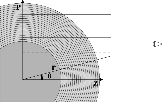
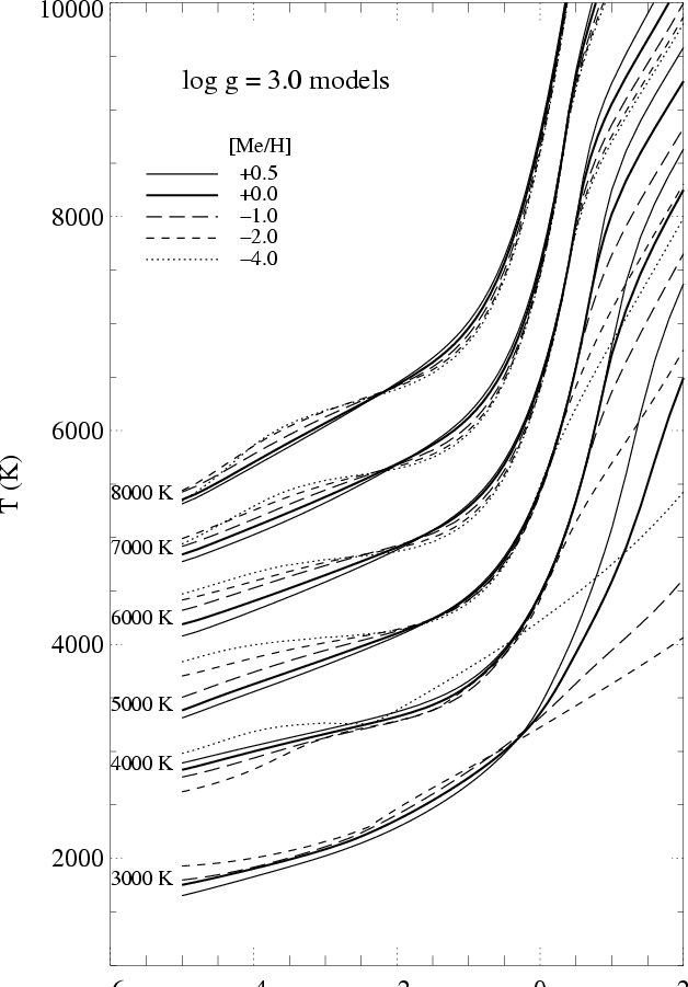
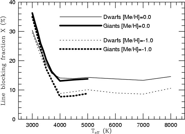
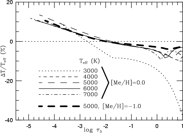
![\begin{figure}
\par\includegraphics[width=8.5cm,clip]{9724fg12.eps}
\end{figure}](/articles/aa/full/2008/30/aa09724-08/img262.gif)
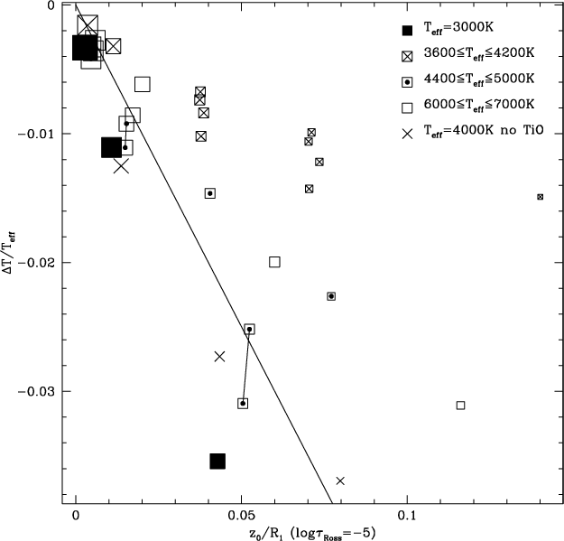
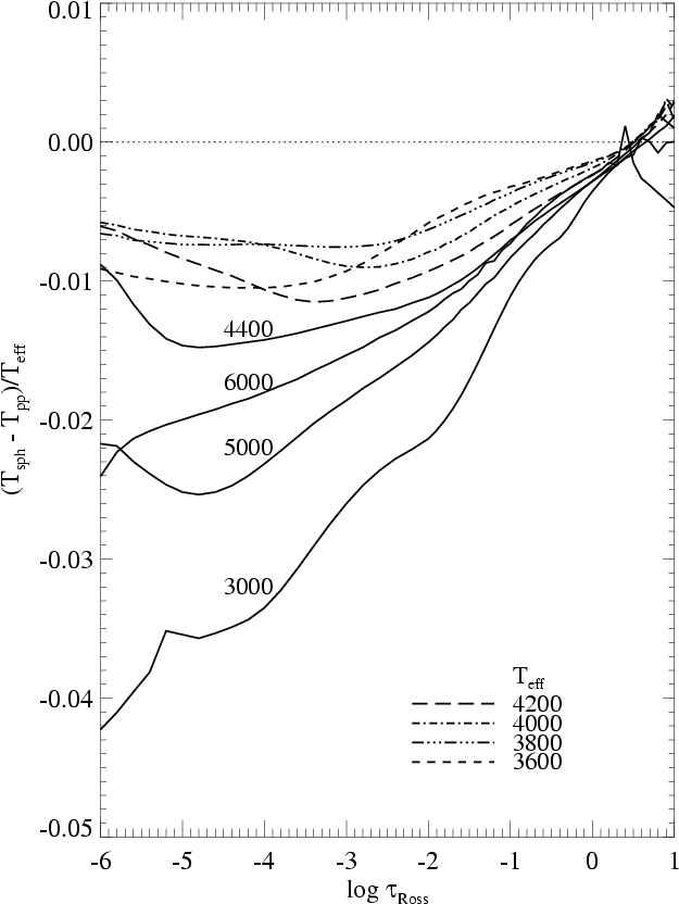
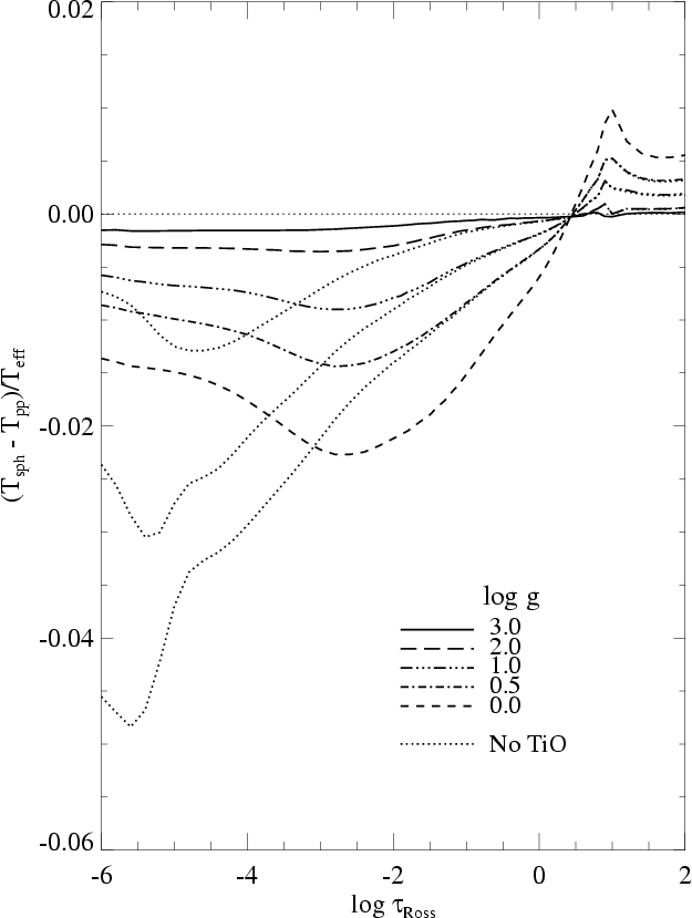
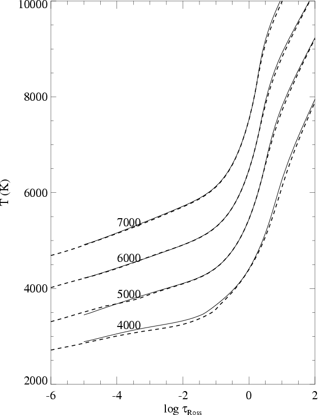
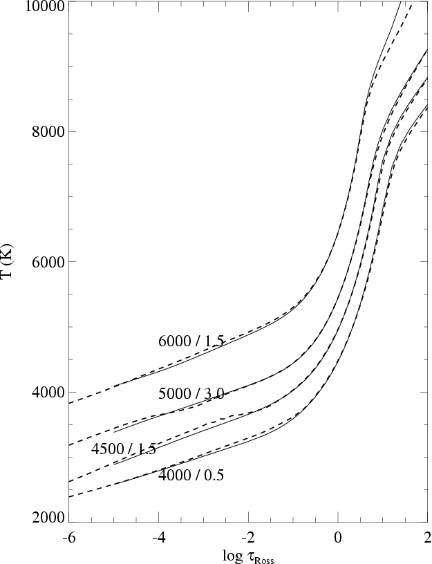
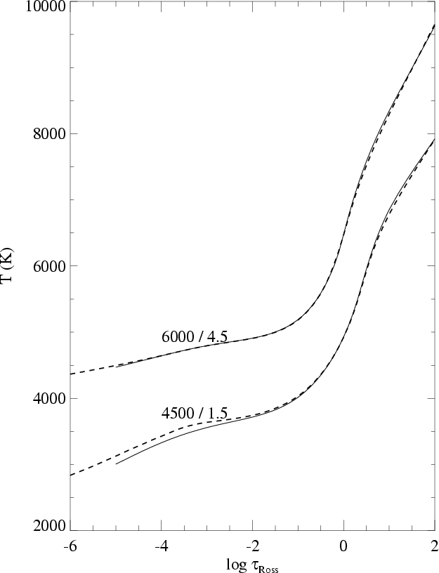
![\begin{figure}
\par\includegraphics[width=8.5cm,clip]{9724fg20.eps}
\end{figure}](/articles/aa/full/2008/30/aa09724-08/img285.gif)