 |
(1) |
A&A 484, 419-428 (2008)
DOI: 10.1051/0004-6361:20078496
T. Aikawa
Tohoku Gakuin University, Izumi-ku, Sendai, 981-3193, Japan
Received 17 August 2007 / Accepted 14 February 2008
Abstract
Context. Linear and also nonlinear pulsation models with the variable Eddington factor approximation of the radiative transfer are constructed.
Aims. The aim of the study is to apply hydrodynamic models of radial pulsation to the observed variability in some post-AGB stars. It has been shown that the pulsation behavior could be strongly effected by the radiative field of the envelope of these stars because of high luminosity in these low mass supergiant stars. Thus, it is important to treat the radiative field with a higher approximation than the diffusion approximation which has been used successfully in classical Cepheids.
Methods. The moment equations of radiative transfer are integrated into the hydrodynamic equations with a variable Eddington factor. The factor is calculated independently by solving the transfer equation of spherical geometry. The linear eigen value problem of the radial perturbation from hydrostatic equilibrium is solved, and nonlinear simulations of radial pulsation are performed with the same approximation of the radiative transfer. The method is applied to pulsation of low mass supergiant stars and, for comparison, classical Cepheids.
Results. The properties of the strange modes that appear often in low mass supergiant star models e.g. post-AGB stars are seriously affected by different treatments of the radiative field in the linear analyses and nonlinear simulations.
Key words: stars: variables: general - radiative transfer
The diffusion approximation of radiative transfer has been used for radial pulsation models of classical cepheids and RR Lyrae variables. The approximation is used for linear analysis and also nonlinear simulation (Castor 1971; Christy 1966a,b) for those stars. For much more luminous stars, however, it is necessary to use higher approximations of the radiative transfer.
The variable Eddington factor approximation for radiative transfer of spherical geometry (Mihalas & Mihalas 1984) is one candidate for this extension. Indeed, it was formulated for stellar pulsation models by Davis (1971) and Karp (1975), and has been applied to nonlinear radial pulsation for classical cepheids (Bendt & Davis 1971).
For these models, the Eddington factor, which is assumed as a constant in the the diffusion approximation, should be a function of the optical depth in plane and spherical geometry, and also is frequency dependent for non-gray atmospheres. The Eddington factor is determined by approximations of the original transfer equations (Unno 1976) or by directly solving the original transfer equation (York 1980).
Davis (1972) applied his radiative models to radial pulsation of W Virginis type stars. While there are no noticeable effects due to different treatments of the radiative transfer on Cepheid models, he pointed out that the diffusion approximation tends to dam up radiation in thin zones, not allowing it to flow freely. Shocks, propagating in thin zones have a tendency to be isothermal, radiating more strongly than they should be. His results suggest that these deficiencies related to shock regions are removed by using radiative transfer models. This comparative study strongly demonstrates the effects of different treatments of radiative transfer.
Fokin (1990) developed a nonlinear pulsation code of radiative transfer which was similar to the one by Davis (1972) and applied it to pulsation of low mass supergiant stars, and in particular, a post AGB star, HD 56126 (Jeannin et al. 1996, 1997).
On the other hand, Chistensen-Dalsgaard & Frandsen (1983) applied radiative transfer models with a variable Eddington factor approximation to a linear analysis of solar oscillations. Zalewski (1991, 1992) developed a linear analysis of radial pulsation with radiative transfer on supergiant stars, and applied the method to linear pulsation of the strange modes for post-AGB stars. He pointed out that the linear growth rates of so-called strange modes that appear with highly excited or damped modes of radial pulsation in linear models of post-AGB stars with the diffusion approximation (Wood 1976; Saio et al. 1984; Aikawa 1991, 1993) change when using radiative transfer for the same model parameters. Thus, comparative studies of different treatments of radiative transfer in linear analysis and nonlinear simulations are necessary.
In this paper, we present linear and nonlinear pulsation models using a unified treatment of radiative transfer. The method will be applied to the pulsation of low mass supergiant stars, particularly strange mode pulsation of post-AGB stars. Some post-AGB stars show photometric variability (see, Van Winckel ). Some of them have long-term observations, i.e. 89 Her and HD 161796 (Fernie 1986; Percy et al. 2000), and pulsation may be responsible for this variability (Lebzelter & Hinkle 2002). Aikawa (1991, 1993) showed that radial pulsation models for luminous low mass supergiant stars have strange modes and nonlinear simulations of these models show irregular oscillations with small amplitudes, which are distinguishing features of the variability of post-AGB stars. The existence of these irregular pulsations may be used to distinguish post-AGB stars from intermediate mass supergiant stars in the spectral types from B to G (Takeda et al. 2007). Moreover, pulsation is sometimes a key to understand the nature of post-AGB stars (Corsico et al. 2007) and post-AGB related stars, for instance, FG Sagittae (Jeffery & Schönberner 2006).
While we are concerned with the effects of radiative transfer on the pulsation behavior in low mass luminous stars, we also construct radiative transfer models for Cepheids for comparison.
The basic hydrodynamic equations for radial pulsation and moment equations of radiative transfer are combined with a variable Eddington factor approximation.
We use the following fundamental equations of radiative
transfer in spherical geometry (York 1980):
|
(1) |
 is the specific intensity along the ray with the direction
cosine
is the specific intensity along the ray with the direction
cosine  and photon frequency
  .
The absorption and scattering
coefficients are
.
The absorption and scattering
coefficients are
 and
and
 ,
and the source
function
,
and the source
function  ,
the phase function for photon scattering
,
the phase function for photon scattering
 .
Thomson scattering and Rayleigh scattering are
included as absorption (Seaton 1993). Scattering due to
dust particles should be included for extended atmospheres, but here
we ignore this effect. The time dependent term is also
ignored as it is of order v/c (Castor 1972).
.
Thomson scattering and Rayleigh scattering are
included as absorption (Seaton 1993). Scattering due to
dust particles should be included for extended atmospheres, but here
we ignore this effect. The time dependent term is also
ignored as it is of order v/c (Castor 1972).
We then use the method of moments for the radiative transfer equations to
combine them with hydrodynamic equations. The resulting moments, to the second
order, are defined as:
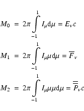
 is the radiation energy density,
 the
net radiation flux,
the
net radiation flux,
 the radiation
pressure tensor, and c is the speed of light and the subscript is photon frequency.
When these moments are introduced into Eq. (1), by integration, we
obtain two equations,
the radiation
pressure tensor, and c is the speed of light and the subscript is photon frequency.
When these moments are introduced into Eq. (1), by integration, we
obtain two equations,
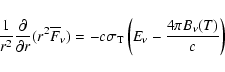 |
(2) |
![\begin{displaymath}c\left[\frac{1}{{r^2 }}\frac{\partial }{{\partial r}}\left(r^...
...nu
-E_\nu }{{r}} \right] = - \sigma _{\rm T} \overline F_\nu
\end{displaymath}](/articles/aa/full/2008/23/aa8496-07/img19.gif) |
(3) |
 ,
and the first term of
,
and the first term of
 is the absorption coefficient corrected for induced
emission, and the second term is due to Thomson scattering and
Rayleigh scattering. The source function is reduced
to
is the absorption coefficient corrected for induced
emission, and the second term is due to Thomson scattering and
Rayleigh scattering. The source function is reduced
to
 as LTE, where
  is the Planck function.
Introducing the variable Eddington factor  as
as
 |
(4) |
and
.
The variable Eddington factor is estimated separately by numerically solving
the original transfer equation with the given source function and
opacities (York 1980), and may vary with limits between 1/3 and 1.
Finally, the Eqs. (2) and (3) are reduced to:
|
(5) |
![\begin{displaymath}c\left[ {\frac{{\partial (f_\nu E_\nu )}}{{\partial r}} + \fr...
... - 1)}}{r}E_\nu} \right] = - \sigma _{\rm T} \overline F_\nu.
\end{displaymath}](/articles/aa/full/2008/23/aa8496-07/img26.gif) |
(6) |
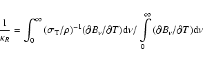
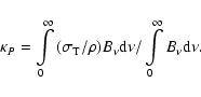
 )
to reduce the frequency-dependent
Eqs. (5) and (6) to frequency-integrated moment equations:
)
to reduce the frequency-dependent
Eqs. (5) and (6) to frequency-integrated moment equations:
 |
(7) |
 |
(8) |
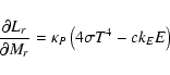
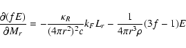
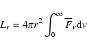
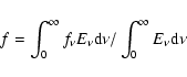
Finally, after dividing by  and integrating over the photon
frequency, we obtain two equations which may be coupled with hydrodynamic
equations:
and integrating over the photon
frequency, we obtain two equations which may be coupled with hydrodynamic
equations:
 |
(9) |
 |
(10) |
 |
(11) |
 |
(12) |
 |
(13) |
 |
(14) |
 |
(15) |
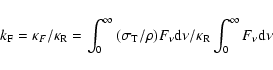
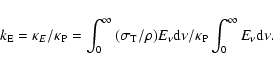
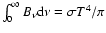
 is the Stefan-Boltzmann constant which appears with
 .
.
 is the ratio of the flux mean to the Rosseland mean, and
 is the ratio of the absorption mean to the Planck mean.
The denominators of the two ratios
are calculated using the Planck function as the spectral density function.
But the other two mean opacities depend on the full nongrey
radiation field. For the first approximation, we assume that the flux
mean is equal to the Rosseland mean, and the absorption mean is equal
to the Planck mean, i.e.
is the ratio of the absorption mean to the Planck mean.
The denominators of the two ratios
are calculated using the Planck function as the spectral density function.
But the other two mean opacities depend on the full nongrey
radiation field. For the first approximation, we assume that the flux
mean is equal to the Rosseland mean, and the absorption mean is equal
to the Planck mean, i.e.
 and
and
 (see Mihalas &
Mihalas 1984, for discussions of this).
f is the frequency-mean Eddington factor.
(see Mihalas &
Mihalas 1984, for discussions of this).
f is the frequency-mean Eddington factor.
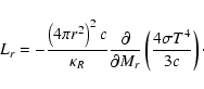
Under the hydrostatic equilibrium i.e.
 and the Eddington
approximation f=1/3, the above equations are reduced to the well-known
expression of the diffusion approximation:
and the Eddington
approximation f=1/3, the above equations are reduced to the well-known
expression of the diffusion approximation:
 |
(16) |
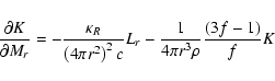
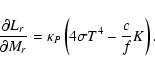
We introduce K = fE, and then we have
 |
(17) |
 |
(18) |
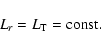
(A) at the bottom of the envelope,
 |
(19) |
 ,
,
 |
(20) |
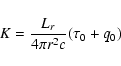
,
and q0 is the Hopf function, evaluated at the optical depth
but we assume a constant,
 .
.
Substituting K in Eqs. (18) to (17) with f=1/3, we can estimate
the difference between the non-equilibrium and equilibrium diffusion
approximation:
 |
(21) |
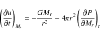
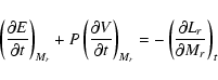
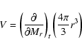
To evaluate the Eddington factor f, we need to solve the radiative transfer equations with the given source function and the opacities (Yorke 1980). Again assuming f=1/3, we obtain radiative hydrodynamics with a non-equilibrium diffusion approximation. The approximation was used in the models by Dorfi & Feuchtinger (1991). In this paper, instead, we numerically solve the radiative transfer equations for a spherical geometry to evaluate the factor. We assume a grey atmosphere with the opacity of a material that may be estimated with the Rosseland mean opacity. We assume that the Eddington factor obtained from the grey atmosphere is equal to f in Eqs. (17) and (18).
 |
(22) |
 |
(23) |
 |
(24) |
 |
(25) |
 |
(26) | ||
 |
(27) |
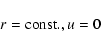
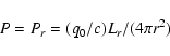
The boundary conditions for these equations are:
at the bottom of the envelope(C)
 |
(28) |
 |
(29) |
In the following, we study radial pulsation of low mass supergiant stars, in particular, pulsation due to the strange mode. We compare this with pulsation in Cepheid models to emphasize the effects on the strange modes. We summarize the model parameters of the two models for a low mass supergiant star and a Cepheid.
For a low mass supergiant (LmSG) star,
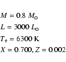
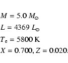
In these models, we ignored the effect of convection, and we used OP opacity (Seaton 1993; Seaton et al. 1994) for Roseland mean and Planck mean opacities. For regions of low density and low temperature, the opacities supplied by Alexander & Ferguson (1994) are used. We use a simplified equation of state: chemical abundances consist of hydrogen (X), helium (Y) and metal abundances (Z). The metal abundances are assumed to be in solar abundance ratios. Then Na, Al are assumed always ionized, and Mg, Si, Fe are treated as a single element and the first ionization is considered. Other elements are ignored.
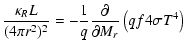
 ,
a constant in the envelope, and from
Eq. (18),
we obtain
,
a constant in the envelope, and from
Eq. (18),
we obtain
 |
(30) |
 |
(31) | ||
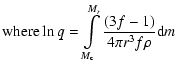 |
 is the mass coordinate of the bottom of the envelope.
We can integrate Eq. (31) starting with the boundary condition at
the surface (B) in which we assume the surface as the location of
the optical depth,
is the mass coordinate of the bottom of the envelope.
We can integrate Eq. (31) starting with the boundary condition at
the surface (B) in which we assume the surface as the location of
the optical depth,
 .
.
Combining this equation with the hydrostatic equilibrium, we can determine the temperature and density distribution in the envelope for a given distribution of the Eddington factor f. Then, we numerically solve the transfer equation for a given source function and opacity distribution. We iterate this process until the iteration reaches a consistent solution starting with the Eddington approximation, i.e., f=1/3.
Figure 1 show the distributions of the factor in the envelope for both the models. Compared with the Cepheid model, the LmSG model has a much wider region where the Eddington factor deviates from f=1/3, and the region reaches just above the top of the hydrogen ionization zone. This feature is important for the behavior of the strange mode pulsation, because the hydrogen ionization zone is responsible for pulsation driving of the mode (Aikawa & Sreenivasan 1985).
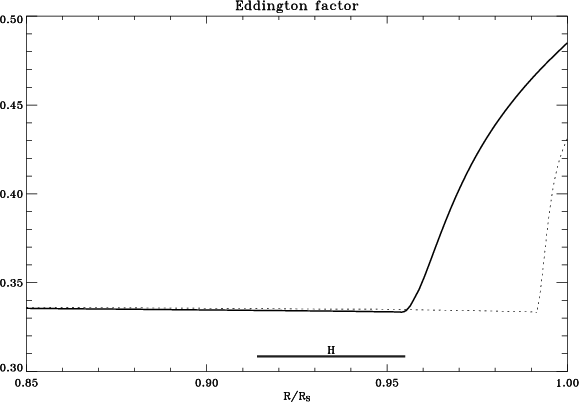 |
Figure 1: The distribution of the Eddington factor in the hydrostatic equilibrium for the models of low mass supergiant stars (thick solid line) and Cepheids (dotted line). The zone of the hydrogen ionization for the former model is indicated with horizontal line. |
| Open with DEXTER | |
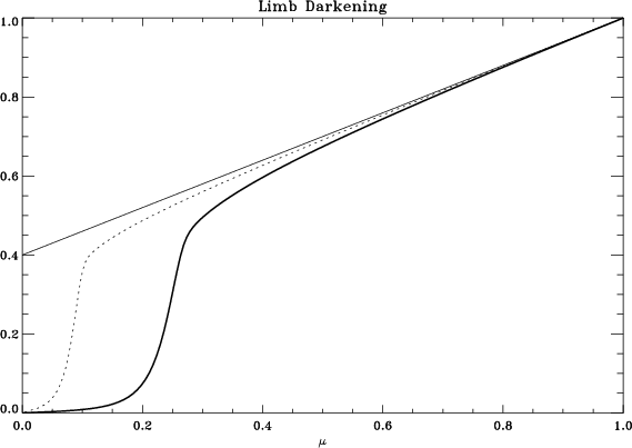 |
Figure 2: The limb darkening of LmSG (thick solid line) and Cepheid (dotted line) models and the Eddington approximation (solid line). |
| Open with DEXTER | |
The distribution of the Eddington factor in the envelope reflects
the limb darkening law at the surface. The Eddington approximation
f=1/3 gives the well-known limb darkening law:
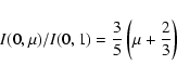 |
(32) |
 is the intensity at the optical depth,
  and the direction cosine
  and
and
 .
.
Figure 2 shows the limb-darkening of the present two models. Except for extreme limb regions, the limb darkening laws of both models coincide with that reached using by the Eddington approximation. The deviation from the Eddington approximation is much greater in LmSGstar model than in the Cepheid model, as expected.
In the following
 denotes the Eddington factor
in equilibrium models.
denotes the Eddington factor
in equilibrium models.
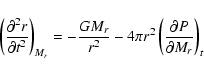
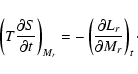
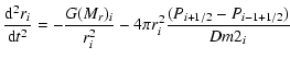
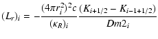
For linear theory, we combine Eqs. (17) and (18) to one equation:
 |
(33) |
 |
(34) |
 |
(35) | ||
| i = 2,3, ...N,N + 1 |
 |
|||
![$\displaystyle -{\frac{{(4\pi r_i^2 )^2 c}}{{(\kappa _R )_i }}}
{\left[ \frac{1}{{4\pi r^3 \rho }}\frac{{(3f - 1)}}{f}K\right]}_i$](/articles/aa/full/2008/23/aa8496-07/img80.gif) |
(36) | ||
| i=2,3,... N |
 |
(37) | ||
| i=1,2,... ,N |
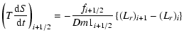 |
(38) | ||
| i=1,2,... ,N |
| Dm1 i+1/2 = (M r) i+1-(M r) i | (39) |
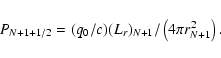
| Dm2 i = (Dm1 i+1/2+Dm1 i-1/2)/2. | (40) |
At the inner boundary:
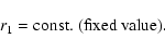 |
(41) |
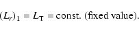 |
(42) |
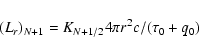 |
(43) |
 |
(44) |
For a linear analysis we assume that we are given a model that is in
hydrostatic equilibrium according to the difference Eqs. (35)-(38) with
time-derivatives set to zero. The infinitesimal deviation of any
variables from their values in the hydrostatic equilibrium will
be indicated by the
prefix  .
We also need
.
We also need
 ,
the Eddington factor
for the perturbation, which might be evaluated by the perturbation on
radiative intensity
,
the Eddington factor
for the perturbation, which might be evaluated by the perturbation on
radiative intensity
 .
We linearize Eqs. (35)-(38) by expanding all
the functions appearing in them in a Taylor series about
the equilibrium model, retaining only terms of zero or first order
in the perturbation. Thus we replace the first order variables as
follows:
.
We linearize Eqs. (35)-(38) by expanding all
the functions appearing in them in a Taylor series about
the equilibrium model, retaining only terms of zero or first order
in the perturbation. Thus we replace the first order variables as
follows:
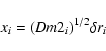 |
(45) |
 |
(46) |
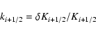 |
(47) |
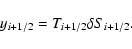 |
(48) |
 |
|||
| ..xN,lN,kN+1/2,yN+1/2,xN+1)T. | (49) |
 for all the perturbations and replace
 by
by  .
The eigen frequency
.
The eigen frequency  is complex in general.
For these variables, we have the following equations:
 |
= | G11,i xi - 1 + G12,i xi + G13,i xi + 1 | |
| + G21,i yi - 1 + 1/2+G22,i yi + 1/2 | (50) | ||
| i = 2,3,... ,N,N + 1 |
| li | = |  |
|
![$\displaystyle +{ BL1_{3,i} x_{i + 1} + BL2_{1,i} y_{i - 1+ 1/2}
+ BL2_{2,i} y_{i + 1/2} } \bigr]$](/articles/aa/full/2008/23/aa8496-07/img100.gif) |
(51) | ||
| i = 2,3,... N |
| ki + 1/2 | = |  |
|
![$\displaystyle \times {({\rm d}R1_{i + 1/2} x_i + {\rm d}R2_{i + 1/2}x_{i + 1} )} \biggr] +
\frac{1}{cK_{i + 1/2} (\kappa _{\rm P})_{i +1/2} }$](/articles/aa/full/2008/23/aa8496-07/img102.gif) |
|||
![$\displaystyle \times \left[ {\frac{(L_{r} )_{i + 1} }{Dm1_{i + 1/2} }l_{i + 1} -
\frac{(L_{r} )_i }{Dm1_{i + 1/2} }l_i } \right]$](/articles/aa/full/2008/23/aa8496-07/img103.gif) |
(52) | ||
| i = 1,2,... ,N |
 |
(53) | ||
| i = 1,2,... ,N. |
![$\displaystyle F = \frac{{(K_{i + 1/2} - K_{i - 1 + 1/2} )}}{{{\rm d}m2_i }} + \left[ {\frac{1}{{4\pi r^3 \rho }}\frac{{(3f - 1)}}{f}K} \right]_i$](/articles/aa/full/2008/23/aa8496-07/img105.gif) |
(54) |
 is the linearly perturbed part of F.
Then we have the eigen value problem with a matrix, M, and the vector,
 :
:
 |
(55) |
 is a band matrix in which the elements are
functions of quantities in hydrostatic equilibrium and the
eigen frequency, .
The band width of this band matrix is 10, if we arrange
linearized Eqs. (50)-(53) in order.
is a band matrix in which the elements are
functions of quantities in hydrostatic equilibrium and the
eigen frequency, .
The band width of this band matrix is 10, if we arrange
linearized Eqs. (50)-(53) in order.
We solve this eigen value problem by iterations. For Cepheids, the eigen values estimated by the quasi-adiabatic approximation will be appropriate for the initial guess of the eigen values. For a luminous low mass supergiant star, however, non-adiabatic effects are so strong that the initial guess of eigen values is useless. Therefore, we adopt the following strategy.
We introduce a control parameter  in Eq. (38):
 |
= | ![$\displaystyle - \epsilon \frac{1}{{Dm1_{i
+ 1/2} }}\left[ {(L_{r} )_{i + 1} - (L_{r} )_i } \right]$](/articles/aa/full/2008/23/aa8496-07/img111.gif) |
(56) |
| i=1,2,... ,N. |
 ,
corresponds
to adiabatic perturbation, and
,
corresponds
to adiabatic perturbation, and
 corresponds to fully
non-adiabatic perturbation.
corresponds to fully
non-adiabatic perturbation.
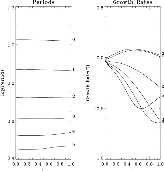 |
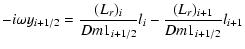
Figure 3:
The pulsation periods (days) and the growth rates as a
function of
for the Cepheid model. |
| Open with DEXTER | |
Equation (55) then is rewritten logically as
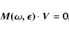 |
(57) |
to 0. For this special case the eigen value problem is complete and
this means we will derive a complete set of eigen values.
We then gradually increase the value of
to 1.
We therefore obtain eigen values that have counterparts in
adiabatic perturbation.
For the Eddington factor, we assume at first
 in the linear
pulsation.
is the Eddington factor for the hydrostatic
equilibrium.
Figure 3 shows the pulsation period and the growth rates for lower
modes as a function of
in the Cepheid model. The
difference of the present results to those obtained by the Eddington
approximation is quite small.
in the linear
pulsation.
is the Eddington factor for the hydrostatic
equilibrium.
Figure 3 shows the pulsation period and the growth rates for lower
modes as a function of
in the Cepheid model. The
difference of the present results to those obtained by the Eddington
approximation is quite small.
Figure 4 shows the results for the LmSG star model. Compared with Fig. 5 obtained for the same model with the diffusion approximation, the positive value of the growth rate of the strange mode, the line of which is labeled 3 in Figs. 4 and 5, is remarkably reduced in this approximation.
As the next problem, we evaluate f in the presence of
the linearly perturbed
quantities. We start with the following equation for perturbed
intensity  which is derived from the Lagrangian perturbed
material quantities:
which is derived from the Lagrangian perturbed
material quantities:
![\begin{displaymath}\mu \frac{{\partial (\delta I)}}{{\partial m_{r} }} + \frac{1...
...- \delta \left[ {\frac{{\kappa (I - S)}}{{4\pi r^2 }}} \right]
\end{displaymath}](/articles/aa/full/2008/23/aa8496-07/img118.gif) |
(58) |
is
the Lagrangian perturbation of the bracket. We ignore the terms
associated with
 .
.
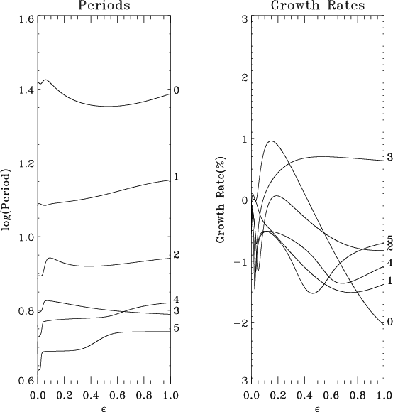 |
Figure 4:
The pulsation periods (days) and the growth rates as a
function of
for the LmSG star model. |
| Open with DEXTER | |
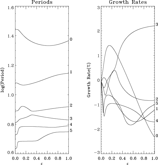 |
Figure 5:
The pulsation periods (days) and the growth rates as a
function of
for the LmSG star model
obtained by using the diffusion approximation. |
| Open with DEXTER | |
Evaluating the bracket, followed by the r-coordinate, we have the
equation for complex :
![$\displaystyle \mu \frac{{\partial (\delta I)}}{{\partial r}} + \frac{{(1 - \mu ...
...(I - S)\frac{{\delta \kappa }}{\kappa } - 2(I - S)\frac{{\delta r}}{r}} \right]$](/articles/aa/full/2008/23/aa8496-07/img122.gif) |
(59) |
where I and S are the mean intensity and source function of the hydrostatic equilibrium model. Thus, we solve the radiative transfer equation of spherical geometry with the complex source function. The boundary conditions of this are the same as used for the equilibrium model.
From ,
we can evaluate the Eddington factor which is complex
in general. We denote this
.
Then we solve the linear eigen value problem using the Eddington
factor
 to obtain the eigen value and the perturbations.
To arrive at consistent solutions, we again require iterations. We solve the
linear problem with an assumed
.
The starting form of the
assumed
is
and then we evaluate f with the
perturbed quantities until a consistent solution is reached.
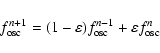
For some cases, the iteration unexpectedly skips between
different modes. Then we take the following strategy:
to obtain the eigen value and the perturbations.
To arrive at consistent solutions, we again require iterations. We solve the
linear problem with an assumed
.
The starting form of the
assumed
is
and then we evaluate f with the
perturbed quantities until a consistent solution is reached.
For some cases, the iteration unexpectedly skips between
different modes. Then we take the following strategy:
 |
(60) |
 is a small factor, about 0.05. Starting
with
is a small factor, about 0.05. Starting
with
 and
and
 which is obtained
from the perturbed quantities with
,
we continue the iteration
until
which is obtained
from the perturbed quantities with
,
we continue the iteration
until
 within the small error. By this
method, we successfully obtain consistent solutions of the
eigen value problem.
within the small error. By this
method, we successfully obtain consistent solutions of the
eigen value problem.
Figure 6 shows the paths of the convergence of the
iteration for the low mass supergiant star model. We
obtain the eigen values up to the 10th modes.
Except for the strange mode, the effects on the periods and the
growth rates of using
are small.
For the strange mode, the present approximation has serious
effects on the pulsation period as well as the growth rate.
We demonstrate in Fig. 7 the distribution of
for the strange
mode in the LmSG model. At the hydrogen ionization zone, it deviates
strongly from
,
the value of the equilibrium model.
We summarized the results of the linear models using various
Eddington factor approximations in Table 1. Compared
with the ordinary modes, the strange mode has remarkably strong
changes for the growth rates and also the periods.
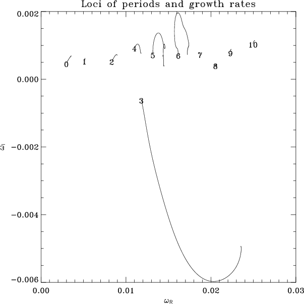 |
Figure 6:
The paths of the convergence of iteration for the model with
for the LmSG model. The paths of the modes, up to the 10th
overtone, are indicated with the label of the mode. The ordinate is
the real part of the eigen value, and the abscissa is the imaginary part. |
| Open with DEXTER | |
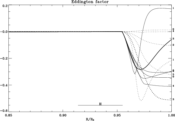 |
Figure 7:
The distribution of the Eddington factor,
(complex),
for various modes for the LmSG model. The real and imaginary parts of
the factor are denoted by solid and dotted lines, respectively. |
| Open with DEXTER | |
Table 1: The periods and the growth rates of the LmSG model.
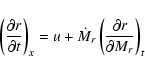
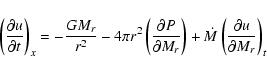
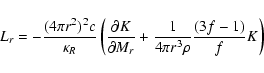
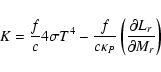
We start nonlinear pulsation models with expressions (17), (18) and (22)-(25). As described in
Eqs. (35)-(38) as the finite difference
expression, these equations may be converted directly to
finite-difference forms. However, dynamic
re-zoning, during which ionization zones and shock regions are confined to
fine zoning regions may reduce the effects of artifacts in the light curves.
So we introduce re-zoning as a diffusion equation on mesh
points. The equations now become:
 |
(61) |
 |
(62) |
 |
(63) |
 |
(64) |
![\begin{displaymath}\left( {\frac{{\partial E}}{{\partial t}}} \right)_{x} + P\le...
...\frac{{\partial V}}{{\partial M_{r} }}} \right)_{t} } \right]
\end{displaymath}](/articles/aa/full/2008/23/aa8496-07/img135.gif) |
(65) |
 denotes
 which is calculated with
algorithms for dynamic re-zoning.
which is calculated with
algorithms for dynamic re-zoning.
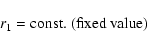
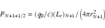
The boundary conditions for these equations are the same in linear pulsation:
At the inner boundary:
 |
(66) |
| u1 = 0 | (67) |
|
(68) |
|
(69) |
 |
(70) |
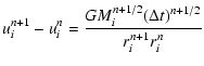
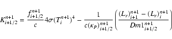
The finite difference scheme that has been used most successfully
is presented in the following equations:
 |
(71) |
 |
|||
![$\displaystyle \qquad +\frac{{2\pi (\Delta t)^{n + 1/2} }}{{3Dm2_i^{n + 1} }}\left[ {(r_i^{n
+ 1} )^2 + r_i^{n + 1} r_i^n + (r_i^n )^2 } \right]$](/articles/aa/full/2008/23/aa8496-07/img142.gif) |
|||
![$\displaystyle \qquad \times\left[ {(p + q)_{i - 1/2}^{n + 1} + (p + q)_{i - 1/2}^n
- (p +q)_{i + 1/2}^{n + 1} - (p + q)_{i + 1/2}^n } \right]$](/articles/aa/full/2008/23/aa8496-07/img143.gif) |
|||
 |
(72) |
![$\displaystyle (L_{r})_i^{n + 1} =
\left( {\frac{{(4\pi (r_i^{n + 1} )^2 )^2 c}}...
... {\frac{1}{{4\pi r^3 \rho }}
\frac{{(3f - 1)}}{f}K} \right)_i^{n + 1} } \right]$](/articles/aa/full/2008/23/aa8496-07/img145.gif) |
(73) |
 |
(74) |
![$\displaystyle E_{i + 1/2}^{n + 1} - E_{i + 1/2}^n + \frac{1}{2}\left[ {(p + q)_{i
+ 1/2}^{n + 1} + (p + q)_{i + /1/2}^n } \right]$](/articles/aa/full/2008/23/aa8496-07/img147.gif) |
|||
 |
|||
 |
|||
![$\displaystyle \qquad{+ (p + q)_{i + 1/2}^{n + 1} \left( {\frac{{V_{i + 1 + 1/2}...
...+ 1/2}^{n + 1} - V_{i - 1 + 1/2}^{n + 1} }}{{Dm2_i^{n + 1} }}} \right)} \Biggr]$](/articles/aa/full/2008/23/aa8496-07/img150.gif) |
(75) |
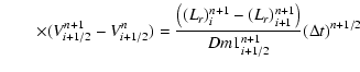
where we introduce the artificial viscosity q to stabilize shock
waves. The formula used is:
![\begin{displaymath}q_{i + 1/2}^n = \frac{{C_{\rm q} }}{{V_{i + 1/2}^n }}\left[ {...
..._{\rm qcut} \sqrt {p_{i + 1/2}^n V_{i + 1/2}^n } )} \right]^2
\end{displaymath}](/articles/aa/full/2008/23/aa8496-07/img151.gif) |
(76) |
 is a parameter to control the amount of
viscosity and
is a parameter to control the amount of
viscosity and
 is another parameter which prevents
unnecessary damping in the deep interior of the envelope (Stellingwerf
1975).
is another parameter which prevents
unnecessary damping in the deep interior of the envelope (Stellingwerf
1975).
Thus we have an implicit difference scheme which guarantees numerical
stability without having to satisfy the Courant-Friedrichs-Lewy condition.
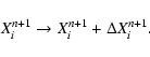
The nonlinear equations are solved,
as usual, by use of the Newton-Raphson technique. We expand
the dependent vector variable as
 |
(77) |
 has a banded
matrix. The band width depends on the arrangement of variables.
We adopt the arrangement of variables as follows:
has a banded
matrix. The band width depends on the arrangement of variables.
We adopt the arrangement of variables as follows:
 |
|||
 |
|||
 |
(78) |
To determine ,
we follow Castor et al.
(1977) and Aikawa & Simon (1985) to keep a certain feature of the
calculation stationary with respect to the mesh. We concentrate on
ionization zones, because the zone should remain in the fine zoning during
pulsation. Otherwise we will have many artifacts in the light curves
that we should compare with observation data. Rezoning is defined
by the equation:
![\begin{displaymath}\left( {\frac{{\partial M_{r} }}{{\partial t}}} \right)_x =
...
...ft[ {Y\frac{{\partial M_{r} }}{{\partial x}}} \right]_{t} + A.
\end{displaymath}](/articles/aa/full/2008/23/aa8496-07/img159.gif) |
(79) |
This equation expresses the diffusive motion of the mesh in the mass coordinate, and is expressed in the finite difference form:
![$\displaystyle M_i^{n + 1} = M_i^n + B_i^n \Delta t^{n + 1}\left[ Y_{i + /12}^n ...
...{i - 1/2}^n (M_i^{n + 1} -
M_{i - 1}^{n + 1} ) \right] +A_i^n \Delta t^{n + 1}.$](/articles/aa/full/2008/23/aa8496-07/img160.gif) |
(80) |
This tri-diagonal matrix for Min + 1 is solved quickly with a given Min, Ain, Bin, and Yi+1/2n. Thus we obtain the instantaneous mass coordinate at the intermediate time between n and n+1 time steps.
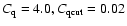
The simulation of the initial value problem is performed using the
values of the static equilibrium except for the velocity profile.
Moreover, this time we use fixed values of the parameters for the
artificial viscosity,
 .
Then
the simulation continues until we obtain stationary states of pulsation,
which are considered as observed states of pulsating stars.
.
Then
the simulation continues until we obtain stationary states of pulsation,
which are considered as observed states of pulsating stars.
The non-linear simulations are performed at first with
,
i.e, the Eddington factor in the non-linear models equal to the one
in the hydrostatic equilibrium. Figure 8 shows light curves at the
photosphere for the Cepheid models.
The simulation is started with velocity profile of the
fundamental mode with a scale factor of -10 km s-1 at the surface, and
the model shows a limit cycle oscillation after a run of
the time interval of about 10 000 days.
The results obtained by using the diffusion approximation are also included.
The light curves obtained without re-zoning,
or with a variable Eddington factor approximation using snapshot
values,
 computed during the simulation, give only minor
changes to the results shown in Fig. 8.
computed during the simulation, give only minor
changes to the results shown in Fig. 8.
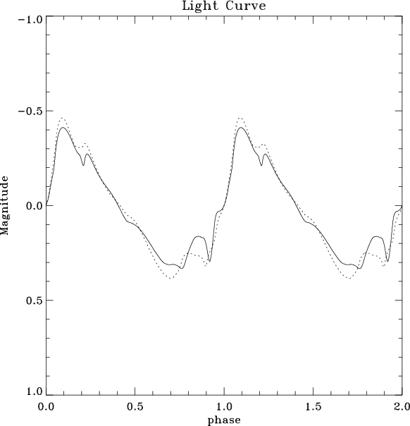 |
Figure 8: The light curves at the photosphere of the Cepheid model by the variable Eddington factor approximation (sold line) and the diffusion approximation (dotted line). |
| Open with DEXTER | |
For the low mass supergiant star model, we first perform the
simulations with the Eddington factor
.
We also used
snapshot values of the factor
evaluated at each time step during the simulation. We denote
the factor as
for this case.
We believe that the simulation using
may correspond
to the linear model with
.
Figure 9 shows the model light curves obtained with different assumptions
on the Eddington factor. It is noted that the differences are
quite effective in changing the light curve of pulsation due to the strange mode.
Figure 10 shows the periodogram of the light curves. It is shown that
the light curve obtained by using the dynamic variable Eddington factor
approximation is sinusoidal with a main period of 3.9 days
and there are no higher components beside the primary component.
On the other hand, the other two light curves are more complicated.
For the model with
,
the period of the main component
is
6.5 days and there are some peaks in their higher harmonics.
For the mode with f=1/3, it seems chaotic pulsation previals,
although there are some peaks at the periods of about 6 days.
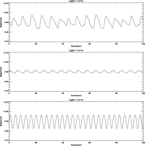 |
Figure 9:
The light curves at the photosphere of the LmSG star model
obtained using the variable Eddington factor approximations:
the diffusion approximation ( top),
( middle) and
( bottom). |
| Open with DEXTER | |
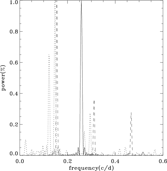 |
Figure 10:
The periodograms of the model light curves. The light curve
obtained using the dynamic variable Eddington factor
approximation (
)
is shown as a solid line. Compared with those
obtained by the
static variable Eddington factor approximation (
)
(dashed line),
and by the diffusion approximation(dotted line), the light curve
obtained by
is quite simple. |
| Open with DEXTER | |
models than in the diffusion models.
Acknowledgements
Part of this work was supported by the Japanese a Grant-in-Aid for Scientific Research of the Ministry of Education, Culture, Sports, science and Technology project number 14540229.