A&A 481, 1-16 (2008)
DOI: 10.1051/0004-6361:20078645
T. Hein - F. Spanier
Lehrstuhl für Astronomie, University of Würzburg, Am Hubland, 97074 Würzburg, Germany
Received 10 September 2007 / Accepted 7 November 2007
Abstract
Context. An analytical solution of the generalized diffusive and convective transport equation is derived to explain the transport of cosmic ray protons within elliptical galaxies.
Aims. Cosmic ray transport within elliptical galaxies is an interesting element in understanding the origin of high energetic particles measured on Earth. As probable sources of those high energetic particles, elliptical galaxies show a dense interstellar medium as a consequence of activity in the galactic nucleus or merging events between galaxies. Thus it is necessary for an appropriate description of cosmic ray transport to take the diffusive and convective processes in a dense interstellar environment into account. Here we show that the transport equations can be solved analytically with respect to the given geometry and boundary conditions in position space, as well as in momentum space.
Methods. From the relativistic Vlasov equation, which is the most fundamental equation for a kinetic description of charged particles within the interstellar medium in galaxies, one finds a generalized diffusion-convection equation in quasilinear theory. This has the form of a ``leaky box'' equation, meaning particles are able to escape the confinement region by diffusing out of the galaxy. We apply here the ``diffusion approximation'', meaning that diffusion in gyrophase and pitch angle are the fastest particle-wave interaction processes. An analytical solution can be obtained using the ``scattering time method'', i.e. separation of the spatial and momentum problems.
Results. The spatial solution is shown using a generalized source of cosmic rays. Additionally, the special case of a jet-like source is illustrated. We present the solution in momentum space with respect to an escape term for cosmic ray protons depending on the spatial shape of the galaxy. For a delta-shape injection function, the momentum solution is obtained analytically. We find that the spectral index measured on Earth can be obtained by appropriately choosing of the strength of Fermi I and Fermi II processes. From these results we calculate the gamma-ray flux from pion decay due to proton-proton interaction to give connection to observations. Additionally we determine the escape-spectrum of cosmic rays. The results show that both spectra are harder than the intrinsic power-law spectrum for cosmic rays in elliptical galaxies.
Key words: acceleration of particles - diffusion - galaxies: elliptical and lenticular, cD
Since their discovery by Viktor Hess in 1912, cosmic rays have been one of the biggest fields of interest in astrophysics, and yet the origin of these particles is still an open question. Fully ionized atomic nuclei reach the Earth coming from outside the solar system with very high energies up to 1020 eV. Most of them with energies <1017 eV seem to originate in the Milky Way, while the highest energetic ones are considered to have an extragalactic origin (for a review see Hoerandel 2007).
The most accepted model for the origin of ultrahigh energy cosmic rays (UHECRs) is acceleration in shock fronts due to Fermi processes (Fermi 1949); hence, the main sources are gamma ray bursts (GRBs), active galaxies like active galactic nuclei (AGN) (Tavecchio 2005), or colliding galaxies. The last two are specially interesting for two reasons. First UHECRs can be generated in elliptical galaxies. Second the increase in the interstellar medium density in objects of these types influences cosmic ray transport (see Bekki & Shioya 1998). But since all elliptical galaxies have an interstellar medium due to star winds, we conclude that the study of transport processes is interesting in general (see Knapp 1999).
In particular, as a result of the GZK-effect, very close AGN are the most probable candidates for UHECR sources (see Biermann 1995). One of these nearby AGN is the giant elliptical galaxy M 87. It is proposed that this galaxy is responsible for acceleration of cosmic ray protons due to Fermi I processes (Rieger et al. 2007; Blandford & Ostriker 1978) in shockfronts within the jet (Reimer et al. 2004). For an overview of proton acceleration in jets (see Mannheim 1993). Since particle acceleration in a jet is located within active galaxies surrounded by an interstellar medium, the high energetic protons undergo physical transport processes before they escape out of the galaxy and reach the detectors on Earth, making a model for cosmic ray transport in elliptical galaxies inevitable. This helps give an answer to the question about the origin of cosmic rays.
Progress has been made in the field of modeling cosmic ray transport with the numerical description of transport processes by Owens & Jokipii (1977) and Strong & Moskalenko (1998). Nevertheless we follow the basic ideas presented in the underlying papers of Lerche & Schlickeiser (1985), Wang & Schlickeiser (1987), and Lerche & Schlickeiser (1988), who used an analytical description of cosmic ray transport. In relation to our work such, a treatment has the following advantages: the model is adequate for cosmic ray transport within any kind of elliptical galaxy including arbitrary cosmic ray sources and the physical parameters involved in our model can be easily fitted to measurements. After all, our analytical model can serve as a test case for more profound numerical models.
In this paper we solve the cosmic ray transport equation analytically with respect to a kinetic description of the interstellar plasma in elliptical galaxies. Special attention is paid to the spatial transport of charged nuclei. In addition, the solution of the momentum equation is derived to explain general properties of this model. As a result, we present illustrative examples of spatial, as well as momentum, cosmic ray transport for given sources of charged nuclei. To show the connection to observations, we calculate the gamma-ray flux from neutral pion decay. These mesons are produced by inelastic scattering processes between cosmic ray protons. The resulting power-law spectrum is slightly harder than the intrinsic one for cosmic rays. Finally, we present the escape spectrum of charged particles leaving elliptical galaxies. Similar to the gamma-ray flux, this spectrum is flatter than the intrinsic one.
To describe the propagation of cosmic ray nuclei within elliptical galaxies, we follow Lerche & Schlickeiser (1985), Lerche & Schlickeiser (1988) and Schlickeiser (2002). For the description of transport processes they use the ``diffusion approximation'', which means that the fastest particle- plasma wave interaction processes are diffusion in gyrophase and pitch angle. Thus following Jokipii (1966), Hasselmann & Wibberenz (1968), and Skilling (1975), we take an isotrope particle distribution function in momentum space. Here we idealise the interstellar medium as a homogeneous volume containing primary cosmic rays being accelerated from the thermal background medium and secondaries resulting from fragmentation of primaries having a negligible abundance in the background medium (cf. Cowsik 1980; Hayakawa 1969).
The transport of these particles at large momenta (p > 10 GeV c-1 nucleus-1) is described by the steady-state transport equation (e.g. Schlickeiser 1983).
Such a treatment is suitable to short timescales of diffusive and convective
processes compared to the dynamical timescale of the galaxy (
![]() years).
This is true in the case
of high energetic particles. We assume a spatial diffusion coefficient K(r) of 1029 cm2 s-1 at p= 1 GeV, which is slightly larger than the value measured in the Milky Way (
years).
This is true in the case
of high energetic particles. We assume a spatial diffusion coefficient K(r) of 1029 cm2 s-1 at p= 1 GeV, which is slightly larger than the value measured in the Milky Way (
![]() cm2, (cf. Schlickeiser 2002) because of diffusive processes being less effective in elliptical galaxies. Consequently we get for protons with TeV-energy a timescale of
cm2, (cf. Schlickeiser 2002) because of diffusive processes being less effective in elliptical galaxies. Consequently we get for protons with TeV-energy a timescale of ![]() 108 years. Furthermore, the dynamical age of the galaxy has to be greater than the timescale of source variability to obtain an appropriate description. This is usually given, since the size of the accretion region onto the central black hole is of the order of a few light-days so that a maximal variability timescale of some days is assumed.
108 years. Furthermore, the dynamical age of the galaxy has to be greater than the timescale of source variability to obtain an appropriate description. This is usually given, since the size of the accretion region onto the central black hole is of the order of a few light-days so that a maximal variability timescale of some days is assumed.
At large momenta, spatial diffusion in turbulent magnetic fields
dominates convection in the galactic wind, so that we find a transport equation for the
phase space density
![]() in spatial coordinates
in spatial coordinates ![]() and in the momentum
coordinate p:
and in the momentum
coordinate p:
A link between spatial and momentum diffusion processes can be seen in the relation
between the two diffusion coefficients
We use the ``scattering time'' method proposed by Sunyaev & Titarchuk (1980)
to get an important class
of exact analytical solutions of Eq. (1) following Wang & Schlickeiser (1987).
This implies, that the spatial and momentum operators can be separated as
Under these conditions, in addition to Eqs. (5) and (6), we can find the
formal mathematical solution of Eq. (1) as a convolution
of the spatial and momentum solution functions
![]() and
M(p) following de Freitas Pacheco (1971):
and
M(p) following de Freitas Pacheco (1971):
The most convenient way to find the formal solution of Eqs. (11) and (15)
is to start with the spatial problem.
As can be seen from Eq. (12), the spatial operator
![]() is of
Sturm-Liouville type (cf. Arfken & Weber 2005) and therefore has a complete eigenfunction system
is of
Sturm-Liouville type (cf. Arfken & Weber 2005) and therefore has a complete eigenfunction system
![]() .
As a consequence, the solution function
.
As a consequence, the solution function
![]() can be expanded in this orthonormal system as
can be expanded in this orthonormal system as
| |
Figure 1: Schematical view of an ellipse with its fundamental properties. |
| Open with DEXTER | |
| |
Figure 2:
Left: gray-shaded plane cuts ellipse leading to a
cut view like the graph on the left-hand side. Right: direction of unit vectors of the variables |
| Open with DEXTER | |
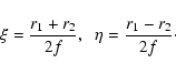
The shape of elliptical galaxies is adjusted to the cosmic
ray transport Eq. (12) using prolate spheroidal coordinates as they are defined by
Abramowitz & Stegun (1972):
Figure 2 shows an illustration of the definition of the three spatial variables ![]() ,
,
![]() ,
and
,
and ![]() .
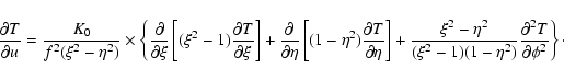
Because of these definitions, we can write Eq. (12) as
.
Because of these definitions, we can write Eq. (12) as
To define reasonable boundary conditions, we assume a ``leaky box'' model. Cosmic ray particles are trapped by disordered magnetic fields within the confinement region of an elliptical galaxy. In this they undergo diffusive and convective movements. At the edge of the box, leakage out of the confinement area is possible.
![\begin{figure}
\par\includegraphics[width=10.3cm,clip]{8645fig3.eps} \end{figure}](/articles/aa/full/2008/13/aa8645-07/img69.gif) |
Figure 3:
Graphic demonstration of the cosmic ray particle density given by the solution
Eq. (30) with the weighting factors (31). The cosmic ray particle density is normalised and given in arbitrary units. As an effect of chosen coordinates
only ``one half'' of the galaxy is visible. For illustration we
plotted
|
| Open with DEXTER | |
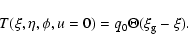
As an illustrative example for spatial boundary conditions, we show
the solution depending on a constant source function over the
elliptical galaxy in Appendix B. To be more specific, we take a
jet-like source function here. The jet points in the direction
![]() (represented by a Dirac delta function) with a length scale chosen to be
(represented by a Dirac delta function) with a length scale chosen to be
![]() for any choice of
for any choice of ![]() being smaller than an arbitrary maximum value of the confinement
region
being smaller than an arbitrary maximum value of the confinement
region
![]() .
Particles leak out at the edge of this region. Such
a boundary condition is known in the literature as a ``free-escape''
condition. For a realistic assumption we decide to let the jet end
smoothly (see the ``Fermi'' function in Eq. (29)). We
neglect any dependence on
.
Particles leak out at the edge of this region. Such
a boundary condition is known in the literature as a ``free-escape''
condition. For a realistic assumption we decide to let the jet end
smoothly (see the ``Fermi'' function in Eq. (29)). We
neglect any dependence on ![]() for an adequate illustration. These
conditions are taken into account by
for an adequate illustration. These
conditions are taken into account by
![\begin{figure}
\par\includegraphics[width=7.5cm,clip]{8645fig4.eps} \end{figure}](/articles/aa/full/2008/13/aa8645-07/img81.gif) |
Figure 4:
Normalised weighting factors |
| Open with DEXTER | |
To get a better understanding of our model, we prove the formal
mathematical solution (Eq. (26)) of the spatial cosmic ray
transport equation. Our discussion is related to the solution found
in the illustrative example in Appendix B, but can similarly done
with Eq. (26):
Second, we show that the sum of solution functions (cf. Eq. (26)), together with the weighting factors in addition
to the given spatial boundary conditions converges. For the
illustrative example in Appendix B, the normalised expansion
coefficients ![]() are shown in Fig. 4. To
obtain applicable results it is essential to include only the first
few ones depending on the requested accuracy.
The resulting solution function is shown in Fig. 5. In the special case of a constant source function, the solution reproduces the boundary condition
are shown in Fig. 4. To
obtain applicable results it is essential to include only the first
few ones depending on the requested accuracy.
The resulting solution function is shown in Fig. 5. In the special case of a constant source function, the solution reproduces the boundary condition
![]() for the variable
for the variable ![]() .
We used
.
We used
![]() for illustration. If we take many eigenfunctions into account, we see at the discontinuity points
for illustration. If we take many eigenfunctions into account, we see at the discontinuity points ![]() and
and
![]() an oscillatory
phenomenon (Gibbs phenomenon). But in this case a closer solution
for the given boundary condition is obtained.
an oscillatory
phenomenon (Gibbs phenomenon). But in this case a closer solution
for the given boundary condition is obtained.
![\begin{figure}
\par\includegraphics[width=7.4cm,clip]{8645fig5.eps} \end{figure}](/articles/aa/full/2008/13/aa8645-07/img89.gif) |
Figure 5:
Spatial solution Eq. (32) in addition with weighting factors |
| Open with DEXTER | |
In analytical calculations, it is a common assumption to include
only the first spatial eigenvalue ![]() .
This one is
associated with the longest escape timescale being the most
important one for modelling escape of particles out of the galaxy.
For numerical purposes, the computing time gives an upper limit to
the possible number of eigenvalues. Furthermore, the spatial
solution as performed in this paper has to match the formal solution
for a spherical geometry within the limit of small ellipticity (
.
This one is
associated with the longest escape timescale being the most
important one for modelling escape of particles out of the galaxy.
For numerical purposes, the computing time gives an upper limit to
the possible number of eigenvalues. Furthermore, the spatial
solution as performed in this paper has to match the formal solution
for a spherical geometry within the limit of small ellipticity (
![]() ). Schlickeiser et al. (1987) found as the spatial solution
). Schlickeiser et al. (1987) found as the spatial solution
For the formal momentum solution, it is
necessary to have a closer look at the spatial solution. As noted
above, the eigenfunction expansion Eq. (19), in addition to
Eq. (20), is indeed the best way to solve the
spatial transport Eq. (11). Inserting this expansion into the
convolution Eq. (10), we can write
As the result of the eigenfunction Eq. (19), we have to
solve one ordinary differential equation for each spatial eigenvalue
instead of the partial differential Eq. (15). Following
Lerche & Schlickeiser (1988), we introduce some simplifying assumptions in order to
find analytic solutions of Eq. (43). We take in
Eq. (16)
![]() ,
,
![]() ,
and
,
and
![]() where p1 is a normalisation value. These
assumptions imply that the most important continuous loss process in
elliptical galaxies at energies >10 GeV is adiabatic energy loss
due to a high galactic wind gradient, whereas pion production losses
are neglected because of the low number density of HI and HII. The
fragmentation lifetime (
where p1 is a normalisation value. These
assumptions imply that the most important continuous loss process in
elliptical galaxies at energies >10 GeV is adiabatic energy loss
due to a high galactic wind gradient, whereas pion production losses
are neglected because of the low number density of HI and HII. The
fragmentation lifetime (![]()
![]() )
is independent of
momentum, and the momentum dependence of the diffusion coefficient
is defined by the parameter s=2-q, where q is the spectral index
of the magnetic turbulence power spectrum. Therefore we get
)
is independent of
momentum, and the momentum dependence of the diffusion coefficient
is defined by the parameter s=2-q, where q is the spectral index
of the magnetic turbulence power spectrum. Therefore we get
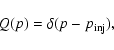
For the special case of a ![]() -function injection of cosmic ray
particles,
-function injection of cosmic ray
particles,
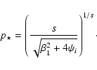
In the case of low values of the momentum (
![]() ), we
find, according to Abramowitz & Stegun (1972),
), we
find, according to Abramowitz & Stegun (1972),
![\begin{figure}
\par\includegraphics[width=8cm,clip]{8645fig6.eps} \end{figure}](/articles/aa/full/2008/13/aa8645-07/img143.gif) |
Figure 6:
Cosmic ray spectrum (grey line) for a delta shape injection at
|
| Open with DEXTER | |
As an illustrative example a spectrum is modelled such that the
result is a power law-spectrum with an exponent like the one
observed from high energetic cosmic rays on Earth. This is
demonstrated in Fig. 6. Here particles are injected
at a momentum value of
![]() with a delta-shape
injection function. Furthermore we assume an isotropic Kolmogorov
turbulence model, i.e., the power law index of the turbulence is
q=5/3. We found a steeper power-law spectrum as the predicted one
from Eq. (54) over about two decades in momentum.
In this regime the exponential cutoff already plays a nonvanishing
role. As the result of the small momentum dependence of the
exponential term in Eq. (51) (
with a delta-shape
injection function. Furthermore we assume an isotropic Kolmogorov
turbulence model, i.e., the power law index of the turbulence is
q=5/3. We found a steeper power-law spectrum as the predicted one
from Eq. (54) over about two decades in momentum.
In this regime the exponential cutoff already plays a nonvanishing
role. As the result of the small momentum dependence of the
exponential term in Eq. (51) (
![]() for Kolmogorov-like turbulence), a power-law spectrum over just two
decades in momentum is obtained. Performing some delta-shape
injections at increasing momenta with adequate normalisation values
a power-law spectrum over a wide range in momentum is obviously
possible.
for Kolmogorov-like turbulence), a power-law spectrum over just two
decades in momentum is obtained. Performing some delta-shape
injections at increasing momenta with adequate normalisation values
a power-law spectrum over a wide range in momentum is obviously
possible.
The parameter that affects the final power-law index of the cosmic
ray spectrum is the parameter a that describes the ratio of energy
gains from the Fermi I process and the Fermi II momentum diffusion
process. To match the -4.8 spectrum from observations, the value
has been chosen as a=250. The adiabatic losses are assumed to be
as strong as the Fermi II energy gains. In this context we need to
remember that the solution function Ri(p) has to be multiplied by
![]() to obtain the number of particles at the momentum p:
to obtain the number of particles at the momentum p:
The reason for this different behavior compared to spiral galaxies is based on the loss time scales. While in the latter the escape loss processes dominate because of the small galactic height compared to the radial size, this is different in elliptical galaxies, where the smallest ``edge'' of the confinement region is given by the semi-minor axis being larger than the galactic height in spirals. Therefore the dominating loss process in elliptical galaxies is adiabatic loss.
The results of the solutions of the transport equations have been explained in the previous section. For astrophysical scenarios it is important to compare these with observations. Here we concentrate on the gamma-ray spectrum due to neutral pion decay and on the escaping cosmic ray spectrum from elliptical galaxies.
The found solutions allow us to calculate the
gamma-ray flux from pion decay. The pions are mainly produced due to
proton-proton interactions, so we concentrate on the reaction
![]() .
The neutral pion decays after
the mean lifetime
.
The neutral pion decays after
the mean lifetime ![]()
![]() 10-17 s in two gamma-photons.
Other interaction channels can be treated analogously. Then the
derivation is straightforward, but tedious.
10-17 s in two gamma-photons.
Other interaction channels can be treated analogously. Then the
derivation is straightforward, but tedious.
We have to convolve the high-energy proton spectrum,
Eq. (26) multiplied with Eq. (52),
with the pion power of a single proton. The latter one is
approximately given by (cf. Schlickeiser 2002; Mannheim & Schlickeiser 1994):
With this result, the differential gamma-ray source function is
given by (cf. Schlickeiser 2002)
Consequently, as discussed before, we assume a power-law spectrum
over a wide range in momentum until a maximum value of
![]() :
:
We next derive the spectrum leaking out of elliptical galaxies.
Therefore the mean free path
![]() for single
scattering events between charged particles and plasma waves is
needed. According to Schlickeiser (2002), this characteristic length is
given by
for single
scattering events between charged particles and plasma waves is
needed. According to Schlickeiser (2002), this characteristic length is
given by
![\begin{figure}
\par\includegraphics[width=9.3cm,clip]{8645fig7.eps} \end{figure}](/articles/aa/full/2008/13/aa8645-07/img186.gif) |
Figure 7:
Schematic view of the geometry for calculating the escape-spectrum
from elliptical galaxies. Particles within the gray-shaded area leave the galaxy by chance,
if their mean free path
|
| Open with DEXTER | |
All particles in the gray-shaded area will escape the galaxy, if
![]() ,
where we
neglect a geometrical factor of order unity. The width of this
spherical shell is constant in every direction so that
,
where we
neglect a geometrical factor of order unity. The width of this
spherical shell is constant in every direction so that
![]() ,
as indicated in
Fig. 7. The rate of the escaping high
energetic particles is approximatively given by the inverse escape
time
,
as indicated in
Fig. 7. The rate of the escaping high
energetic particles is approximatively given by the inverse escape
time
Under these conditions we can convert Eq. (72) into
Such an effect can be easily understood by the high energetic
particles leaving the galactical confinement region more frequently
than low energetic ones. As a consequence there are two
possibilities explaining the observed high energy cosmic ray
spectrum above the ``knee'' with spectral index of -3.1 assuming
that elliptical galaxies provide a significant amount to the overall
high-energy cosmic ray flux. First, the intrinsic spectrum in
elliptical galaxies may be steeper then that one we have chosen
here. In this context the measurement of the gamma-ray flux reaching
the Earth from such an object would give us interesting constraints.
Second, if the intrinsic spectrum in elliptical galaxies has nearly
the same dependence as the one we measure here on Earth
(
![]() ), the transport of cosmic rays after escape
from elliptical galaxies depends on energy. In these two scenarios
it is possible to explain the high-energy component with our model.
), the transport of cosmic rays after escape
from elliptical galaxies depends on energy. In these two scenarios
it is possible to explain the high-energy component with our model.
Note that, due to the previously given arguments, the highest
energetic particles cannot be confined within the galactical volume.
In our examination the maximum energy of confined charged particles
within elliptical galaxies is given by the relation
We showed that an analytical treatment of cosmic ray transport in elliptical galaxies based on the diffusion approximation is possible in general. The formal solution we found, combined with appropriate boundary conditions and source functions, can be used to study transport processes in elliptical galaxies. This model is valid for the complete physical parameter space as long as the diffusion approximation holds.
The first test case where we applied our model to is a jet-like injection shape like in M 87. As we can separate our problem into spatial and momentum problems, this test case probes the spatial problem. For this model we found that for very long timescales cosmic rays are distributed throughout the galaxy almost isotropically. We also provided a test case for the momentum problem. Under the assumption of a resulting power-law spectrum matching the observed power law-spectrum on Earth, we could identify the governing eigenfunctions and therefore the governing processes for cosmic ray acceleration and momentum diffusion in elliptical galaxies. It turned out that in elliptical galaxies adiabatic losses are responsible for the high energy cutoff, whereas the slope of the spectrum is given by the ratio of the strength of Fermi I and Fermi II processes. As a result of the basic possibility of explaining this power law-with physical parameters that might be found in M 87, our calculation gives rise to the theory of M 87 as a source of ultra-high energy cosmic rays. In this context the gamma-ray flux from pion decay and the escaping cosmic ray spectrum are essential for a more adequate view of cosmic ray astrophysics. We find that the gamma-ray spectrum with a power law index of -2.69 is a bit harder than the intrinsic cosmic ray spectrum (power law index -2.8). In the context of understanding the sources of high-energy cosmic rays, the flux of charged particles escaping from the confinement region of elliptical galaxies is also very interesting. For the same intrinsic spectrum as above, we find -2.13 as the spectral index for escaping particles. Again the spectrum is harder than the value within elliptical galaxies.
Our model may also serve as a testbed for some more advanced questions:
Nevertheless this work is considered as a starting point for more sophisticated (numerical) models. Another interesting point is the expansion of this model to cosmic ray electrons. While the spatial description may be derived analogously, we need to add the physical processes involved in the transport of electrons in momentum space. Synchrotron losses and the inverse Compton effect will then play a major role (see, e.g., Casadei & Bindi 2004). The output of this model can be easily tested with the radio data of elliptical galaxies since the electrons provide the main contribution to this radiation.
Acknowledgements
T.H. acknowledges support by Graduiertenkolleg 1147 and F.S. acknowledges support by the Deutsche Forschungsgemeinschaft, DFG project number Sp 1124/1-1. We would like to thank R. Schlickeiser for his useful comments.
The general solution of Eq. (25) can be obtained by
consecutive separation of variables. First we use
Equation (79) can be solved through another separation of
variables. With
Equation (90) has the formal mathematical solution given by
Under these conditions we can write the formal mathematical solution
as
As an illustrative example we calculate the solution depending on
the following boundary conditions. First we define one for the
variable ![]() .
Remembering, that
.
Remembering, that ![]() is equal to the semi-major
axis a we assume ``free escape'' boundary conditions in the form
is equal to the semi-major
axis a we assume ``free escape'' boundary conditions in the form
In order to match Eq. (96) only even solution functions
are practical. This is done by
![]() .
Therefore we
neglect
.
Therefore we
neglect
![]() having singularities at the points
having singularities at the points ![]() and
and ![]() .
From Eq. (95) we recognise that
.
From Eq. (95) we recognise that
![]() if
if
![]() .
Let yri be the
zeros of
.
Let yri be the
zeros of
![]() ,
then we find
,
then we find
Adjusting Eq. (26) to the boundary condition
Eq. (96) it becomes clear that only even values of rmatch the required periodicity. Using the orthonormality relation
for Legendre polynomials
![\begin{displaymath}%
\mathcal{L}_{\vec{r}}(\vec{r},p) \equiv \nabla \left[K(\vec{r},p)\nabla \right]
\end{displaymath}](/articles/aa/full/2008/13/aa8645-07/img17.gif)
![\begin{displaymath}%
\mathcal{L}_{p}(\vec{r},p) \equiv p^{-2} \frac{\partial}{\p...
...ain}}-p^2\dot{p}_{{\rm loss}}\right]
-\frac{1}{\tau_{\rm c}}
\end{displaymath}](/articles/aa/full/2008/13/aa8645-07/img20.gif)


![\begin{displaymath}%
\mathcal{O}_p=\frac{1}{p^2} \frac{\partial}{\partial p} \le...
...ght]-
\frac{a_4}{\theta_4(p)};\hspace{0.2cm}
h(p)=\kappa(p)
\end{displaymath}](/articles/aa/full/2008/13/aa8645-07/img43.gif)
![\begin{displaymath}%
T(\xi,\eta,u=0)=q_0\frac{\delta(\xi-\xi_{\rm c})\delta(\eta_{{\rm inj}}-\eta)}
{\left[\exp(4(f-f_{{\rm max}})+1\right]}\cdot
\end{displaymath}](/articles/aa/full/2008/13/aa8645-07/img75.gif)
![\begin{displaymath}%
E_{i,r}(\vec{r}) \equiv
T(\xi,u)=\sum_{i=1}^{\infty}\sum_{r...
...\exp \left[ -\frac{K_0 y_{ir}^2}{\xi_{\rm c}^2 f^2}u \right ].
\end{displaymath}](/articles/aa/full/2008/13/aa8645-07/img76.gif)
![\begin{displaymath}%
\alpha_{ir}=\frac{q_0
P_r^0(\eta_{{\rm inj}})}{\exp\left[4(...
...i_{\rm c}^2}{2}\left[ J_{r+\frac{3}{2}}(y_{ir})\right]^2}\cdot
\end{displaymath}](/articles/aa/full/2008/13/aa8645-07/img77.gif)
![\begin{displaymath}%
T(\xi,u)=\sum_{i=1}^{\infty}\alpha_i
\frac{1}{\sqrt{\xi}}J_...
...ht)
\exp \left[ -\frac{K_0 y_i^2}{\xi_{\rm c}^2 f^2}u \right ]
\end{displaymath}](/articles/aa/full/2008/13/aa8645-07/img82.gif)
![\begin{displaymath}%
\alpha_i=\frac{q_0
\int_1^{\xi_g}\xi^{3/2}J_{\frac{1}{2}}\l...
...c{\xi_{\rm c}^2}{2}\left[ J_{\frac{3}{2}}(y_i)\right ]^2}\cdot
\end{displaymath}](/articles/aa/full/2008/13/aa8645-07/img83.gif)
![\begin{displaymath}%
Z(c_i\xi)\,\includegraphics[width=1.2cm]{eq1}\, \frac{1}{c_i\xi}\cos
\left(c_i\xi-\frac{1}{2}\pi \right).
\end{displaymath}](/articles/aa/full/2008/13/aa8645-07/img96.gif)
![\begin{displaymath}%
Z(c_iR)\,\includegraphics[width=1.2cm]{eq2}\, \frac{1}{c_iR}\cos
\left(c_iR-\frac{1}{2}\pi \right),
\end{displaymath}](/articles/aa/full/2008/13/aa8645-07/img100.gif)
![\begin{displaymath}%
\frac{p_{1}^{s}}{p^{2+s}} \frac{\partial}{\partial p} \left...
...}{p^{s}} +\lambda_{i}^{2} \right] R_{i}=-Q(p)p^{-s}
p_{1}^{s}.
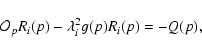
\end{displaymath}](/articles/aa/full/2008/13/aa8645-07/img111.gif)
![$\displaystyle (a_2p_1^s)^{-1}\frac{\Gamma\left[\frac{a+3}{2s}+\frac{\xi_1-[(3+a...
...} \times
p^a \exp\left[-\frac{\beta_1+(\beta_1^2+4\psi_i)^{1/2}}{2s}p^s
\right]$](/articles/aa/full/2008/13/aa8645-07/img114.gif)
![$\displaystyle \times\left\{U\left[\frac{a+3}{2s}+\frac{\xi_1-[(3+a)/2]\beta_1}{...
..._i)
^{1/2}},\frac{a+3}{s},\frac{(\beta_1^2+4\psi_i)^{1/2}}{s}p^s\right]
\right.$](/articles/aa/full/2008/13/aa8645-07/img115.gif)
![$\displaystyle \left.\times\int_0^pdp_0~p_0^{s+1}Q(p_0)\exp\left[\frac{\beta_1-(\beta_1^2+4\psi_i)^{1/2}}{2s}
p_0^s\right] \right.$](/articles/aa/full/2008/13/aa8645-07/img116.gif)
![$\displaystyle \left. \times~
M\left[\frac{a+3}{2s}+\frac{\xi_1-[(3+a)/2]\beta_1...
...)
^{1/2}},\frac{a+3}{s},\frac{(\beta_1^2+4\psi_i)^{1/2}}{s}p_0^s\right] \right.$](/articles/aa/full/2008/13/aa8645-07/img117.gif)
![$\displaystyle \left.+~M\left[\frac{a+3}{2s}+\frac{\xi_1-[(3+a)/2]\beta_1}{s(\be...
..._i)
^{1/2}},\frac{a+3}{s},\frac{(\beta_1^2+4\psi_i)^{1/2}}{s}p^s\right]
\right.$](/articles/aa/full/2008/13/aa8645-07/img118.gif)
![$\displaystyle \left.\times\int_p^{\infty}dp_0~p_0^{s+1}Q(p_0)\exp\left[\frac{\beta_1-(\beta_1^2+4\psi_i)^{1/2}}{2s}
p_0^s\right] \right.$](/articles/aa/full/2008/13/aa8645-07/img119.gif)
![$\displaystyle \left. \times~
U\left[\frac{a+3}{2s}+\frac{\xi_1-[(3+a)/2]\beta_1...
...
^{1/2}},\frac{a+3}{s},\frac{(\beta_1^2+4\psi_i)^{1/2}}{s}p_0^s\right]\right\}.$](/articles/aa/full/2008/13/aa8645-07/img120.gif)


![$\displaystyle \times\left\{M\left[\frac{a+3}{2s}+\frac{\xi_1-[(3+a)/2]\beta_1}{...
...eft[\frac{\beta_1+(\beta_1^2+4\psi_i)^{1/2}}{2s}
p_{{\rm inj}}^s\right] \right.$](/articles/aa/full/2008/13/aa8645-07/img128.gif)
![$\displaystyle \left. \times
~U\left[\frac{a+3}{2s}+\frac{\xi_1-[(3+a)/2]\beta_1...
...frac{a+3}{s},\frac{(\beta_1^2+4\psi_i)^{1/2}}{s}p_{{\rm inj}}^s\right]\right\},$](/articles/aa/full/2008/13/aa8645-07/img129.gif)
![$\displaystyle \times\left\{U\left[\frac{a+3}{2s}+\frac{\xi_1-[(3+a)/2]\beta_1}{...
...eft[\frac{\beta_1+(\beta_1^2+4\psi_i)^{1/2}}{2s}
p_{{\rm inj}}^s\right] \right.$](/articles/aa/full/2008/13/aa8645-07/img131.gif)
![$\displaystyle \left. \times
~M\left[\frac{a+3}{2s}+\frac{\xi_1-[(3+a)/2]\beta_1...
...frac{a+3}{s},\frac{(\beta_1^2+4\psi_i)^{1/2}}{s}p_{{\rm inj}}^s\right]\right\}.$](/articles/aa/full/2008/13/aa8645-07/img132.gif)
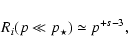
![\begin{displaymath}%
R_i(p \gg p_{\star}) \propto
p^{\frac{a-3}{2}+\frac{a+3}{2}...
...[
-\frac{\beta_1+(\beta_1^2+4\psi_i)^{1/2}}{2s}p^s\right]\cdot
\end{displaymath}](/articles/aa/full/2008/13/aa8645-07/img140.gif)
![\begin{displaymath}%
R_i\left( p \gg (s/\beta_1)^{1/s}\right)=p^{+a-\xi_1/\beta_1}
\exp\left[ -\frac{\beta_1}{s}p^s\right].
\end{displaymath}](/articles/aa/full/2008/13/aa8645-07/img142.gif)
![\begin{displaymath}%
P_{\pi}(\gamma_{\pi},\gamma_{p},\xi,\eta,\phi)=
c\gamma_{\p...
...i}-\gamma_{p}^{3/4})H\left[\gamma_p-\gamma_{{\rm thr}}\right].
\end{displaymath}](/articles/aa/full/2008/13/aa8645-07/img151.gif)
![$\displaystyle \frac{1}{\gamma_{\pi}m_{\pi}c^2}\int_1^{\infty}~{\rm d}\gamma_p T...
...eft[
-\frac{\beta_1+(\beta_1^2+4\psi_i)^{1/2}}{2s}(m_{p}c)^s\gamma_{p}^s\right]$](/articles/aa/full/2008/13/aa8645-07/img159.gif)
![$\displaystyle \times
U\left[\frac{a+3}{2s}+\frac{\xi_1-[(3+a)/2]\beta_1}{s(\bet...
...,\frac{a+3}{s},\frac{(\beta_1^2+4\psi_i)^{1/2}}{s}(m_{p}c)^s\gamma_{p}^s\right]$](/articles/aa/full/2008/13/aa8645-07/img160.gif)
![$\displaystyle 4\pi(m_pc)^{a+2}
\times(a_2p_1^s)^{-1}\frac{\Gamma\left[\frac{a+3...
...1}\exp\left[\frac{\beta_1+(\beta_1^2+4\psi_i)^{1/2}}{2s}
p_{{\rm inj}}^s\right]$](/articles/aa/full/2008/13/aa8645-07/img163.gif)
![$\displaystyle \times ~
M\left[\frac{a+3}{2s}+\frac{\xi_1-[(3+a)/2]\beta_1}{s(\b...
...{1/2}},\frac{a+3}{s},\frac{(\beta_1^2+4\psi_i)^{1/2}}{s}p_{{\rm inj}}^s\right].$](/articles/aa/full/2008/13/aa8645-07/img164.gif)
![$\displaystyle \frac{4}{3}\frac{T^2(\xi,\eta,\phi)\sigma_{0,pp}^{\pi^0}}{m_{\pi
...
...-\frac{\beta_1+(\beta_1^2+4\psi_i)^{1/2}}{2s}(m_{p}c)^s\gamma_{p}^{4s/3}\right]$](/articles/aa/full/2008/13/aa8645-07/img166.gif)
![$\displaystyle \times
U\left[\frac{a+3}{2s}+\frac{\xi_1-[(3+a)/2]\beta_1}{s(\bet...
...ma_{p}^{4s/3}\right]\times
H\left[\gamma_{\pi}-\gamma_{{\rm thr}}^{3/4}\right].$](/articles/aa/full/2008/13/aa8645-07/img167.gif)
![$\displaystyle \gamma_{\pi}^{4a/3+3}(\gamma_{\pi}^{4/3}-1)^{0.53}\exp\left[
-\frac{\beta_1+(\beta_1^2+4\psi_i)^{1/2}}{2s}(m_{p}c)^s\gamma_{p}^{4s/3}\right]$](/articles/aa/full/2008/13/aa8645-07/img173.gif)
![$\displaystyle \times
U\left[\frac{a+3}{2s}+\frac{\xi_1-[(3+a)/2]\beta_1}{s(\bet...
...{a+3}{s},\frac{(\beta_1^2+4\psi_i)^{1/2}}{s}(m_{p}c)^s\gamma_{p}^{4s/3}\right],$](/articles/aa/full/2008/13/aa8645-07/img174.gif)
![\begin{displaymath}%
N(\gamma_p)=N_0\gamma^{-z}H\left[\gamma_{{\rm p,~max}}-\gamma_p
\right].
\end{displaymath}](/articles/aa/full/2008/13/aa8645-07/img176.gif)
![\begin{displaymath}%
Q_{\pi^0}(\gamma_{\pi},\xi,\eta,\phi)=\frac{4}{3}\frac{T^2(...
...right]
H\left[\gamma_{{\rm p,~max}}^{3/4}-\gamma_{\pi}\right].
\end{displaymath}](/articles/aa/full/2008/13/aa8645-07/img177.gif)
![\begin{displaymath}%
Q_{\gamma}(E_{\gamma},\xi,\eta,\phi)\simeq
\frac{8}{3}\frac...
...max}}^{-z+0.78}-\gamma_{{\rm min}}^
{-4/3z+1.04}\right)\right]
\end{displaymath}](/articles/aa/full/2008/13/aa8645-07/img180.gif)
![\begin{displaymath}%
\frac{K(\vec{r},p)}{r^2(\xi,\eta,\phi)}=\frac{c\lambda_{{\rm mfp}}(p)}{3f^2\left[(\xi\eta)^2+(\xi^2-1)(1-\eta^2)\right]},
\end{displaymath}](/articles/aa/full/2008/13/aa8645-07/img189.gif)
![\begin{displaymath}%
N(p)\propto4\pi
p^2\int_0^{2\pi}\int_{-1}^{1}\int_{d_1}^{r_...
...\xi^2-1)(1-\eta^2)\right]}f^2{\rm d}f
{\rm d}\eta {\rm d}\phi.
\end{displaymath}](/articles/aa/full/2008/13/aa8645-07/img190.gif)
![\begin{displaymath}%
N\propto 4\pi
p^2\int_{0}^{2\pi}\int_{-1}^{1}\int_{r_{\rm g...
...^2+(\xi^2-1)(1-\eta^2)\right]}{\rm d}f{\rm d}\eta
{\rm d}\phi.
\end{displaymath}](/articles/aa/full/2008/13/aa8645-07/img193.gif)


![\begin{displaymath}%
-\frac{1}{B}\frac{\partial^2 B}{\partial \phi^2}=
\frac{(\x...
...tial A}{\partial \eta}\right]\right\}
+(\xi^2-1)(1-\eta^2)c^2.
\end{displaymath}](/articles/aa/full/2008/13/aa8645-07/img208.gif)

![\begin{displaymath}%
\frac{(\xi^2-1)(1-\eta^2)}{(\xi^2-\eta^2) \times A}
\left\{...
...right]\right\}+\left\{(\xi^2-1)(1-\eta^2)c^2-m^2\right\}A = 0.
\end{displaymath}](/articles/aa/full/2008/13/aa8645-07/img210.gif)
![\begin{displaymath}%
\frac{\partial}{\partial \xi}\left[(\xi^2-1)\frac{\partial
...
...2
\left(\frac{1}{\xi^2-1}+\frac{1}{1-\eta^2}\right)\right]A=0.
\end{displaymath}](/articles/aa/full/2008/13/aa8645-07/img213.gif)
![\begin{displaymath}%
\frac{\partial}{\partial \xi}\left[(\xi^2-1)\frac{\partial
...
...ight]-\left(\beta_{mn}-\xi^2c^2+\frac{m^2}{\xi^2-1}\right)R=0,
\end{displaymath}](/articles/aa/full/2008/13/aa8645-07/img215.gif)
![\begin{displaymath}%
\frac{\partial}{\partial \eta}\left[(1-\eta^2)\frac{\partia...
...ht]+\left(\beta_{mn}-\eta^2c^2-\frac{m^2}{1-\eta^2}\right)S=0.
\end{displaymath}](/articles/aa/full/2008/13/aa8645-07/img216.gif)
![\begin{displaymath}%
\int_0^a J_{\nu}\left( \alpha_{\nu u}
\frac{\rho}{a}\right)...
...\rho = \frac{a^2}{2}[J_{\nu
+1}^2(\alpha_{\nu u})]\delta_{uw},
\end{displaymath}](/articles/aa/full/2008/13/aa8645-07/img249.gif)
![\begin{displaymath}%
E_i(\vec{r}) \equiv T(\xi,u)=\sum_{i=1}^{\infty}\alpha_i
\f...
...ht)
\exp \left[ -\frac{K_0 y_i^2}{\xi_{\rm c}^2 f^2}u \right ]
\end{displaymath}](/articles/aa/full/2008/13/aa8645-07/img251.gif)
![\begin{displaymath}%
\alpha_i=\frac{q_0
\int_1^{\xi_{\rm g}}\xi^{3/2}J_{\frac{1}...
...c{\xi_{\rm c}^2}{2}\left[ J_{\frac{3}{2}}(y_i)\right ]^2}\cdot
\end{displaymath}](/articles/aa/full/2008/13/aa8645-07/img252.gif)