 |
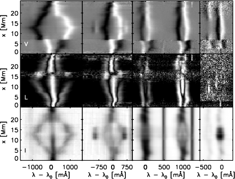
Figure 1: Stokes profiles along the symmetry line connecting spot center and disc center. The limb side is down, the center side up. Bottom row: intensity, I. Middle row: total linear polarization, L. Top row: circular polarization, V. Left to right: IR spectral lines at 1564.8 nm, 1565.2 nm, visible lines at 630.15 nm, 630.25 nm, and Ti I at 630.37 nm. |
| Open with DEXTER | |
In the text
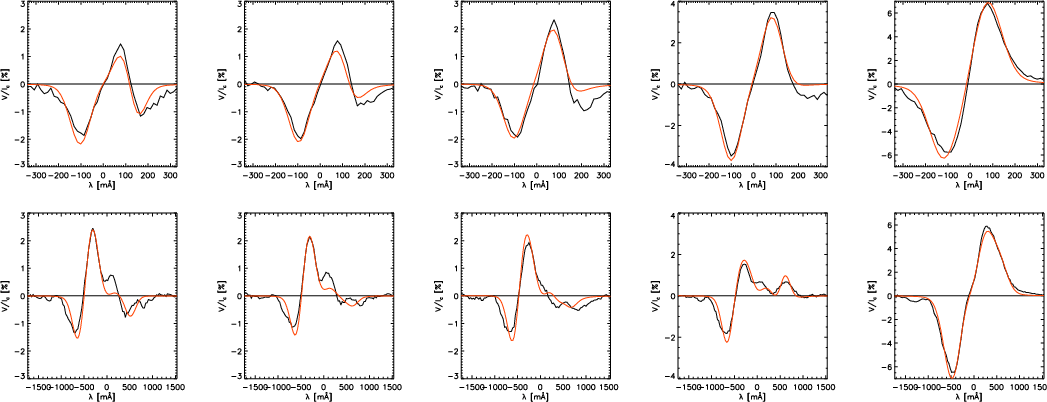 |
Figure 2: Examples of Stokes V profiles in the neutral line. Top row: Stokes V of the Fe I line at 630.15 nm. Bottom row: the co-spatial profiles of Fe I at 1564.8 nm. The red line gives the corresponding best-fit profile of the inversion. The last column shows a profile in the center side penumbra. |
| Open with DEXTER | |
In the text
| |
Figure 3: Continuum intensity maps of NOAA 10425 in the near infrared on 2003 August 7 ( left) and August 9 ( right). The distance between tick marks is 1 arcsec. |
| Open with DEXTER | |
In the text
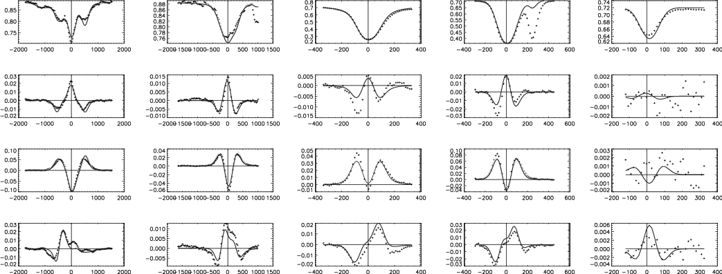 |
Figure 4: Comparison of the observed (+) and best-fit profiles ( solid line) for one spatial position in the neutral line of Stokes V. Left to right: IR lines at 1564.8 nm and at 1565.2 nm; visible lines at 630.15 nm, 630.25 nm, and 630.37 nm. Top to bottom: Stokes IQUV as a fraction of the continuum intensity. The black vertical lines mark the zero wavelength of the respective wavelength scales. The dispersion on the x-axis is in mÅ for all spectra. |
| Open with DEXTER | |
In the text
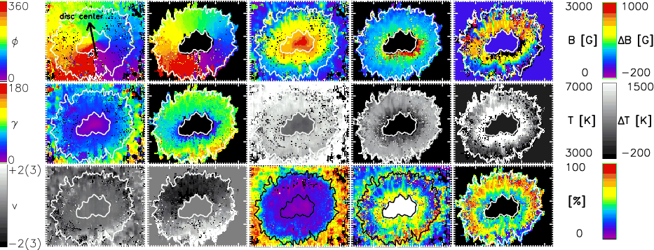 |
Figure 5: Top row, left to right: magnetic field azimuth of the background component (bg), field azimuth of the flow-channel component (fc), field strength of bg, field strength of fc, and difference of the field strengths (bg-fc). Middle row, left to right: field inclination of bg and fc, temperature of bg and fc, difference of temperatures (bg-fc). Bottom row, left to right: LOS velocity of bg and fc, stray light contribution, filling fraction of bg and fc. Inclination and azimuth are given in the LRF frame; velocities are in km s-1 with negative velocities pointing towards the observer. The velocity limits in parentheses refer to the fc component. White contour lines denote the inner and outer boundary of the penumbra. The black arrow in the azimuth map points towards disc center. |
| Open with DEXTER | |
In the text
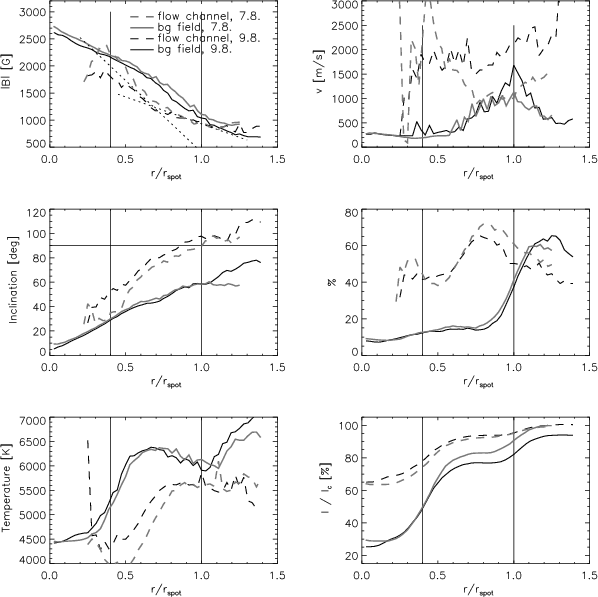 |
Figure 6:
Left column, top to bottom: radial variation of B, LRF
inclination, temperature at log |
| Open with DEXTER | |
In the text
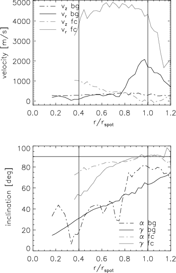 |
Figure 7:
Top: horizontal and vertical velocities for both inversion
components. Black: bg component. Grey: fc component.
Dashed: vertical velocity. Solid: horizontal velocity.
Bottom: field inclination, |
| Open with DEXTER | |
In the text
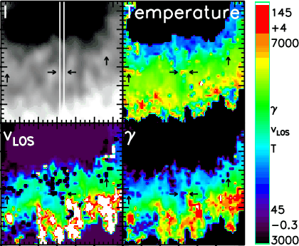 |
Figure 8: Top row: continuum intensity and temperature of the fc component. Bottom row: velocity and inclination of the fc component. The white lines mark the column, along which the parameters shown in Fig. 9 were taken. Black arrows point towards hot upstreams in the mid penumbra. |
| Open with DEXTER | |
In the text
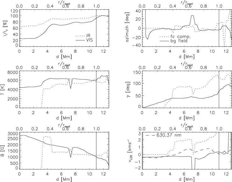 |
Figure 9: Parameters along the column marked in Fig. 8. Left column, top to bottom: continuum intensity, temperature, field strength. Right column, top to bottom: field azimuth, field inclination, LOS velocity. In all graphs besides intensity, solid lines indicate quantities of the bg field and dotted lines those of the fc component. For intensity, solid and dotted correspond to visible, respectively, IR continuum intensity. The LOS velocity of Ti I is given by the long-dashed line in the velocity graph. The vertical black line marks the outer penumbral boundary. The second hot upstream intersected by the cut at d=6.2 Mm has a similar signature in all quantities as the upflows at the inner penumbral boundary. |
| Open with DEXTER | |
In the text
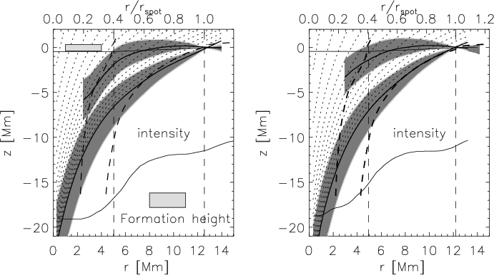 |
Figure 10:
Integrated inclination of the data from August 7 (
left) and August 9 ( right). Lower thick black line: bg
component; upper thick black line: fc component. Dark grey
shaded: same curve including inclination variations.
Thick dashed lines: the boundary layers of the spot model of JS94. Thin black line: radial variation of the IR continuum intensity. Vertical dashed lines: inner and
outer penumbral boundary. The thin black line at around z=0 km
marks the location of the |
| Open with DEXTER | |
In the text
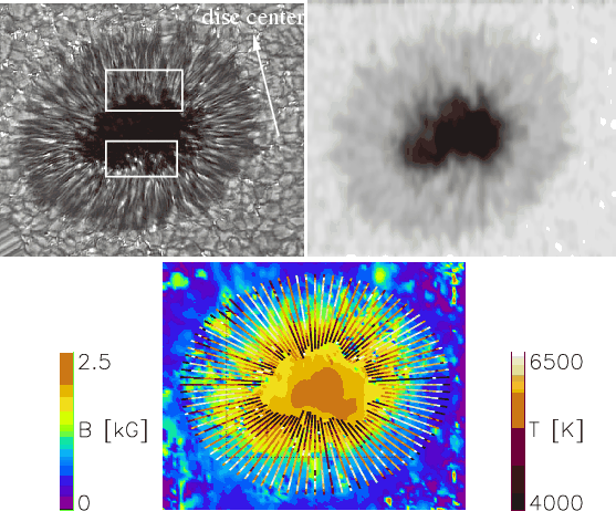 |
Figure 11: Top left: image of NOAA 10425 in the G-band from the DOT on La Palma, taken on August 9 about half an hour after the observations at the VTT. The white arrow points towards disc center. The white rectangles mark regions with an identically structured umbra-penumbra boundary in both intensity maps. Top right: IR continuum map. Bottom: top view of the 3D model. See text for the description. |
| Open with DEXTER | |
In the text
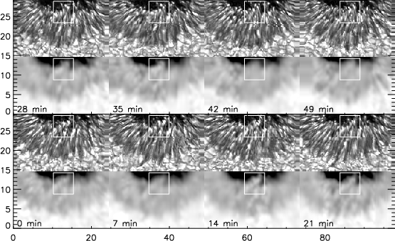 |
Figure 12: The temporal evolution of the penumbra with 7 min cadence. Data of NOAA 10425 on 2003 August 9. The lower row shows the IR continuum intensity, the upper row the co-temporal and co-spatial map in the G-band from the DOT. Tick marks are arcsec; time increases from left to right in each row. |
| Open with DEXTER | |
In the text
| |
Figure 13: The effects of the inclined LOS on observations of the limb or center side. Thick black: integrated LRF inclination of the 2-component inversion as in Fig. 10, fc component (upper line) and bg component (lower line). The LOS is overplotted in purple for the center side and in orange for the limb side. |
| Open with DEXTER | |
In the text
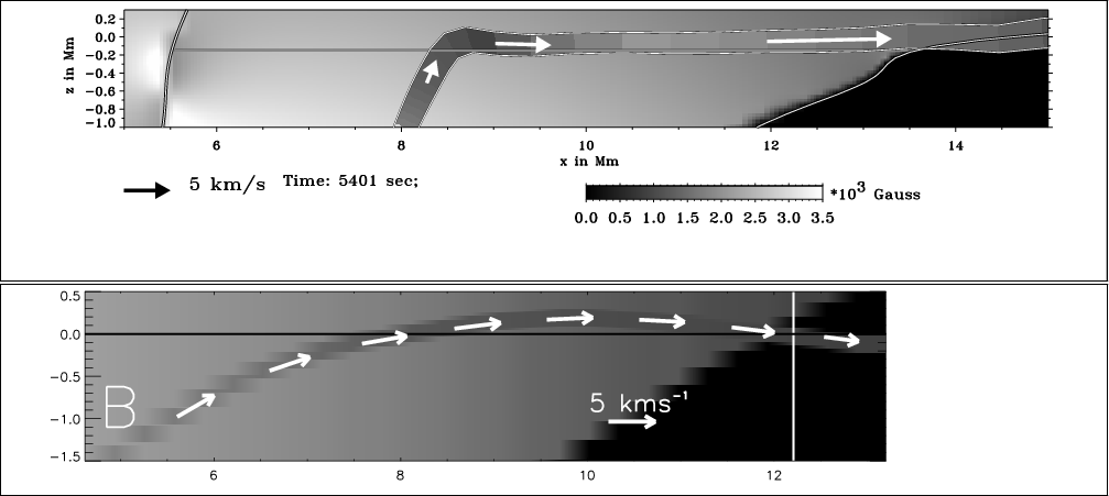 |
Figure 14: Comparison of a snapshot of the moving tube model ( top panel, courtesy of R. Schlichenmaier) with the flow channels' geometry from the observation ( lower panel). The plots have been arranged to have the same scaling and position in the horizontal axis that gives the distance from the spot center in Mm. Both panels display the fc component and the bg component with their respective field strength as color coding. The color bar gives the color coding for the field strength in both graphs. Velocities are overplotted as arrows, whose length gives the absolute velocity. The direction of the arrows for the lower plot is the field inclination. |
| Open with DEXTER | |
In the text
| |
Figure 15: Schematical model of the sunspot structure. |
| Open with DEXTER | |
In the text
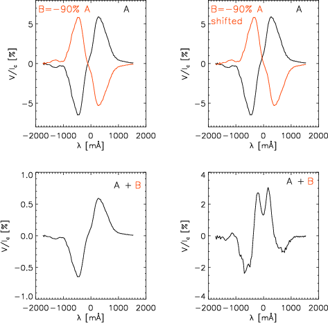 |
Figure A.1: A simple method of producing peculiar V profiles. The addition of the two profiles A and B in the top row yields the profiles in the bottom row. Left column: profile B equals -90% of A and is located at the same wavelength. Right column: B equals -90% of A, but now shifted in wavelength. |
| Open with DEXTER | |
In the text
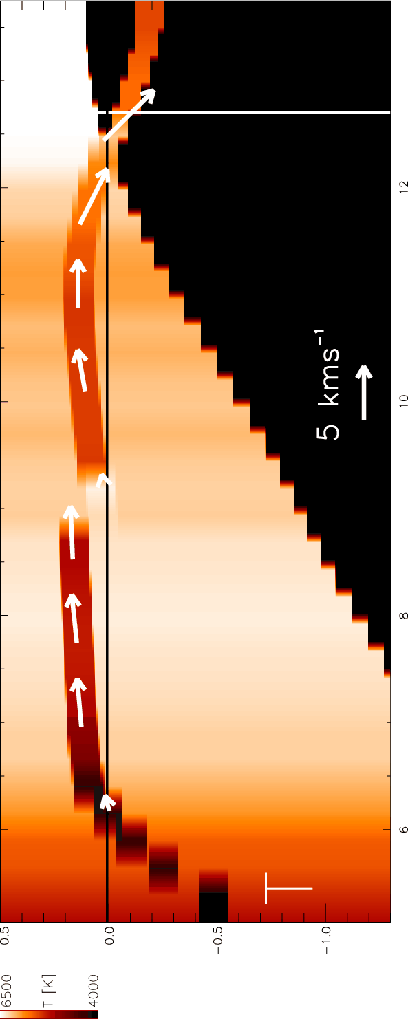 |
Figure B.1: The integrated inclination values along the single column marked in Fig. 8. Similar to Fig. 14, but using temperature for the color coding. The integrated curve has been shifted down at x = 7 Mm, where the hot upstream appears. |
| Open with DEXTER | |
In the text
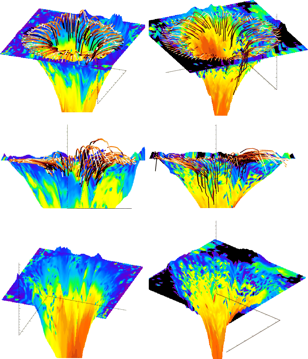 |
Figure B.2: The 3D models from the integration of the inclinations to the surface averaged over 4 degree bins. Left column: data of August 9. Right column: data of August 7. Top to bottom: view from above, side view, view from below. The color coding is identical to Fig. 11. The plot of the flow channels was switched off for the view from below. |
| Open with DEXTER | |
In the text
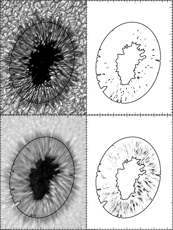 |
Figure C.1: Overview of the DOT data set. Top row: single intensity image ( left) with corresponding mask of brightenings ( right). Bottom row: temporal averages over the time series. The black contours outline the area considered to be the penumbra. Tick marks are in arcsec. |
| Open with DEXTER | |
In the text
| |
Figure C.2: Average histogram of penumbral intensities in the time series. |
| Open with DEXTER | |
In the text
| |
Figure C.3: Autocorrelation functions of the intensity in the penumbra and a quiet Sun reference area. |
| Open with DEXTER | |
In the text