A&A 478, 155-162 (2008)
DOI: 10.1051/0004-6361:20078328
Accretion funnels onto weakly magnetized young stars
N. Bessolaz1 - C. Zanni1 - J. Ferreira1 - R. Keppens2,3,4 - J. Bouvier1
1 - Laboratoire d'Astrophysique de Grenoble, Université
Joseph Fourier, CNRS UMR5571, France
2 -
Centre for Plasma Astrophysics, K.U. Leuven, Belgium
3 -
FOM Institute for Plasma Physics, Rijnhuizen, The Netherlands
4 -
Astronomical Institute, Utrecht University, The Netherlands
Received 20 July 2007 / Accepted 11 November 2007
Abstract
Aims. We re-examine the conditions required to steadily deviate an accretion flow from a circumstellar disc into a magnetospheric funnel flow onto a slow rotating young forming star.
Methods. New analytical constraints on the formation of accretion funnels flows due to the presence of a dipolar stellar magnetic field disrupting the disc are derived. The Versatile Advection Code is used to confirm these constraints numerically. Axisymmetric MHD simulations are performed, where a stellar dipole field enters the resistive accretion disc, whose structure is self-consistently computed.
Results. The analytical criterion derived allows to predict a priori the position of the truncation radius from a non perturbative accretion disc model. Accretion funnels are found to be robust features which occur below the co-rotation radius, where the stellar poloidal magnetic pressure becomes both at equipartition with the disc thermal pressure and is comparable to the disc poloidal ram pressure. We confirm the results of Romanova et al. (2002, ApJ, 578, 420) and find accretion funnels for stellar dipole fields as low as 140 G in the low accretion rate limit of
 .
With our present numerical setup with no disc magnetic field, we found no evidence of winds, neither disc driven nor X-winds, and the star is only spun up by its interaction with the disc.
.
With our present numerical setup with no disc magnetic field, we found no evidence of winds, neither disc driven nor X-winds, and the star is only spun up by its interaction with the disc.
Conclusions. Weak dipole fields, similar in magnitude to those observed, lead to the development of accretion funnel flows in weakly accreting T Tauri stars. However, the higher accretion observed for most T Tauri stars (
 )
requires either larger stellar field strength and/or different magnetic topologies to allow for magnetospheric accretion.
)
requires either larger stellar field strength and/or different magnetic topologies to allow for magnetospheric accretion.
Key words: accretion, accretion disks - magnetohydrodynamics (MHD) - methods: numerical - stars: pre-main sequence
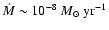
Classical T-Tauri stars (CTTS) are magnetically active, show evidence for circumstellar accretion discs, and can have mean
photospheric magnetic field magnitudes around 1 kG
(e.g. Johns-Krull et al. 1999). Such a strong stellar field is enough to disrupt the inner accretion disc,
provided that one really measures the large scale magnetic field and
not only local strong multipolar components from starspots. However,
this does not seem to be the case since recent polarimetric measurements
(Valenti & Johns-Krull 2004) indicate a weak dipolar component lower than 200 G.
Moreover, observations show evidence for non-direct accretion.
Inverse P-Cygni profiles with strong redshift absorption wings are
indicative of polar accretion near free-fall velocities along
magnetospheric field lines from the inner disc edge
(Bouvier et al. 2003; Edwards et al. 1993; Bouvier et al. 1999).
Although the magnetic field structure of these stars is probably
complex (Gregory et al. 2006), dynamical models of star-disc
interaction usually assume an aligned dipole
field, to simplify the analytical work. Under this assumption, stellar
field lines threading the Keplerian disc below the co-rotation
radius
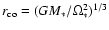 ,
where
,
where  is the stellar angular velocity, would lead to a spin-up of the star,
versus those beyond
is the stellar angular velocity, would lead to a spin-up of the star,
versus those beyond
 ,
to a spin-down. The radial extent of
angular momentum exchange between the star and the disc is then
determined by (1) the disc truncation radius
,
to a spin-down. The radial extent of
angular momentum exchange between the star and the disc is then
determined by (1) the disc truncation radius  ,
where the magnetic
dipole diverts the radially accreting flow to funnel flows; and (2) an
outer radius
,
where the magnetic
dipole diverts the radially accreting flow to funnel flows; and (2) an
outer radius
 beyond which no more stellar field lines are
connected to the disc. In this framework, a star-disc interaction
occurring on a large radial extension (as proposed by Armitage & Clarke 1996; Cameron & Campbell 1993; Ghosh & Lamb 1979), may lead to a disc-locking situation where the star
remains at a slow rotation rate,
despite accretion. On the other hand, it has been argued that this scenario is
unlikely, since the stellar field lines would be opened up by
differential rotation until severing this causal link
(Matt & Pudritz 2005; Lovelace et al. 1995; Aly & Kuijpers 1990, for a recent discussion on that issue).
The outcome of this latter scenario would be a star-disc interaction
limited to a small radial extension around the disc truncation radius.
Many theoretical models then assume that the disc inner edge should be
close to the co-rotation radius (Königl 1991; Shu et al. 1994) for the sake of
angular momentum equilibrium.
beyond which no more stellar field lines are
connected to the disc. In this framework, a star-disc interaction
occurring on a large radial extension (as proposed by Armitage & Clarke 1996; Cameron & Campbell 1993; Ghosh & Lamb 1979), may lead to a disc-locking situation where the star
remains at a slow rotation rate,
despite accretion. On the other hand, it has been argued that this scenario is
unlikely, since the stellar field lines would be opened up by
differential rotation until severing this causal link
(Matt & Pudritz 2005; Lovelace et al. 1995; Aly & Kuijpers 1990, for a recent discussion on that issue).
The outcome of this latter scenario would be a star-disc interaction
limited to a small radial extension around the disc truncation radius.
Many theoretical models then assume that the disc inner edge should be
close to the co-rotation radius (Königl 1991; Shu et al. 1994) for the sake of
angular momentum equilibrium.
For a decade, many numerical works have investigated the star-disc
interaction issue (Hayashi et al. 1996; Kuker et al. 2003; Long et al. 2005).
However, the formation of accretion curtains seems
difficult to reproduce. Although Miller & Stone (1997) found such
polar accretion in the case of a kG dipolar stellar field
associated with a disc field in the same direction to the latter,
Romanova et al. (2002) were the first to demonstrate magnetospheric accretion
along stellar field lines for kG pure dipolar field in axisymmetric simulations
and next by performing 3D simulations (Romanova et al. 2003).
In this paper, we address the issue of the disc truncation radius and
its localisation as a function of the disc (accretion rate) and stellar
(dipole field) parameters. In Sect. 2 we provide analytical
constraints for driving steady accretion funnels and derive an estimate of the
position of the truncation radius. We then use numerical MHD
simulations in Sect. 3 to verify this prediction. We confirm
magnetospheric accretion for a slowly rotating star with an inner
disc hole and a weak stellar magnetic field compatible with observations
of weak accretors.
For a given accretion disc model, predicting where the truncation by the
stellar magnetosphere will occur is an important issue.
Different estimates were given in the literature.
We consider here a pure dipolar field with a strength at the stellar surface in the equatorial
plane equal to B*.
A first dimensional estimate expresses the truncation radius
in the form
 where the Alfvén radius
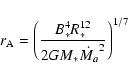 |
(1) |
is a characteristic length which can be derived by equating the ram pressure of a free-falling
spherical envelope with the magnetic pressure of a dipolar field (Elsner & Lamb 1977).
Different estimates of the adimensional coefficient k have been
given in the literature, ranging from
0.5 (Königl 1991; Ghosh & Lamb 1979; Long et al. 2005) to  1 (Ostriker & Shu 1995; Wang 1996; Arons 1993).
A second criterion (Armitage & Clarke 1996; Cameron & Campbell 1993; Matt & Pudritz 2005, and references therein) states
that accretion funnels will take place when the magnetic torque due to
the stellar field matches the "viscous'' or turbulent torque, namely
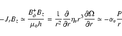 |
(2) |
where
 is the toroidal field at the disc surface,
h the disc scale height, P the disc pressure and
is the toroidal field at the disc surface,
h the disc scale height, P the disc pressure and
 the Shakura & Syunyaev (1973) parameter.
This criterion (hereafter A) gives an upper limit for the truncation radius, as it only defines a radius where the star-disc interaction starts to affect accretion. This maximal truncation radius
the Shakura & Syunyaev (1973) parameter.
This criterion (hereafter A) gives an upper limit for the truncation radius, as it only defines a radius where the star-disc interaction starts to affect accretion. This maximal truncation radius
 occurs when the plasma beta, defined as
 ,
becomes
,
becomes
 where
where
 is a measure of the magnetic
shear and
is a measure of the magnetic
shear and
 is the disc aspect ratio. In a thin Keplerian
accretion disc, one gets
is the disc aspect ratio. In a thin Keplerian
accretion disc, one gets
 at
since q is
close to unity to avoid opening of the magnetosphere (e.g. Matt & Pudritz 2005).
at
since q is
close to unity to avoid opening of the magnetosphere (e.g. Matt & Pudritz 2005).
A third criterion represents a more conservative approach, and gives only a lower limit
 .
It states that accretion funnels take place when accretion is no longer possible because of the overwhelming field strength.
It is usually written (Romanova et al. 2002; Koldoba et al. 2002)
.
It states that accretion funnels take place when accretion is no longer possible because of the overwhelming field strength.
It is usually written (Romanova et al. 2002; Koldoba et al. 2002)
 |
(3) |
where v is the total speed. Note that this criterion
is not predictive since we cannot calculate a priori the dominant
azimuthal velocity  as it is itself an outcome of
the star-disc interaction. Nevertheless, if one wishes to provide an
estimate of the truncation radius, then we can use instead
as it is itself an outcome of
the star-disc interaction. Nevertheless, if one wishes to provide an
estimate of the truncation radius, then we can use instead
 ,
where
,
where
 and a negligible thermal
pressure (both approximations are valid in a thin disc). This will be
our criterion B. At the truncation radius estimated as such, the
plasma beta is
and a negligible thermal
pressure (both approximations are valid in a thin disc). This will be
our criterion B. At the truncation radius estimated as such, the
plasma beta is
 .
.
From the previous discussion, it appears quite obvious that
 is a better approximation for .
The stellar magnetic field, which is bound to become dominant in the magnetosphere, must first favour accretion, i.e. the magnetic torque must be negative. If this is not the case, namely if
is a better approximation for .
The stellar magnetic field, which is bound to become dominant in the magnetosphere, must first favour accretion, i.e. the magnetic torque must be negative. If this is not the case, namely if
 ,
the disc material is radially expelled. This is the "propeller''
regime as studied e.g. by Ustyugova et al. (2006) and references therein.
Accretion thus implies
,
the disc material is radially expelled. This is the "propeller''
regime as studied e.g. by Ustyugova et al. (2006) and references therein.
Accretion thus implies
 ,
with stellar
magnetic field lines as leading spirals. Below co-rotation, accretion
will proceed quite naturally thanks to both the viscous and the
stellar torques. There are then two more independent constraints that
must be fulfilled to produce steady funnel flows.
First, the accretion flow must be prevented by the presence of the magnetosphere. The simplest way to express this is to require that the magnetic poloidal pressure balances the accretion ram pressure
,
with stellar
magnetic field lines as leading spirals. Below co-rotation, accretion
will proceed quite naturally thanks to both the viscous and the
stellar torques. There are then two more independent constraints that
must be fulfilled to produce steady funnel flows.
First, the accretion flow must be prevented by the presence of the magnetosphere. The simplest way to express this is to require that the magnetic poloidal pressure balances the accretion ram pressure
 .
This defines a radius
.
This defines a radius
 where
where
 |
(4) |
where
 is the sonic Mach number measured at the disc midplane.
Now, at radii
is the sonic Mach number measured at the disc midplane.
Now, at radii
 ,
accretion is mainly
due to the stellar torque and
,
accretion is mainly
due to the stellar torque and
 :
material is accreting to the star much faster than in
the outer accretion disc.
Second, material at the disc midplane must be lifted and loaded onto
the stellar field lines. With a dipole field configuration, such a vertical motion can only be due to a vertical
thermal plasma pressure gradient. It therefore requires that the magnetic field
compression is not too strong. This leads naturally to an equipartition,
(as already proposed by Aly 1980; Pringle & Rees 1972).
:
material is accreting to the star much faster than in
the outer accretion disc.
Second, material at the disc midplane must be lifted and loaded onto
the stellar field lines. With a dipole field configuration, such a vertical motion can only be due to a vertical
thermal plasma pressure gradient. It therefore requires that the magnetic field
compression is not too strong. This leads naturally to an equipartition,
(as already proposed by Aly 1980; Pringle & Rees 1972).
One important point to note is that once a large scale magnetic field is close to equipartition in an accretion disc, it is able to deviate a large fraction of the disc plasma from its radial motion to a vertical one.
This has been shown with the calculations of magnetized accretion-ejection structures by Ferreira & Pelletier (1995) and confirmed by numerical MHD simulations (Zanni et al. 2007; Casse & Keppens 2002).
In one sense, making funnel flows involves the same physics as loading mass in magnetized jets.
In fact, almost all of the disc mass can be lifted and loaded onto the field lines when
,
depending mostly on the field bending (see Fig. 3 in Ferreira & Pelletier 1995).
This is why we assume, for finding a simple analytical criterion, that the disc truncation radius
is close to the radius where
,
namely
 .
Using the above estimates, we derive the following two constraints:
.
Using the above estimates, we derive the following two constraints:
 |
(5) |
that must be fulfilled in order to provide steady state funnel
flows. For a dipole field, this translates into a theoretical truncation radius
 |
(6) |
where the stellar field B* has been normalised to 140 G, disc
accretion rate  to 10-8
  yr-1, stellar
mass to 0.8
and stellar radius to 2
yr-1, stellar
mass to 0.8
and stellar radius to 2  .
Note that these are all typical values for CTTS while the chosen value of the magnetic stellar field
B* is consistent with observations of dipole fields in such objects (see Bouvier et al. 2007; Valenti & Johns-Krull 2004, and references therein).
It is clear that the conditions given by Eq. (5) state that the accretion speed close to the base of the accretion funnel is of the order of the Alfvén speed. Indeed Eq. (6)
can be rewritten as
.
Note that these are all typical values for CTTS while the chosen value of the magnetic stellar field
B* is consistent with observations of dipole fields in such objects (see Bouvier et al. 2007; Valenti & Johns-Krull 2004, and references therein).
It is clear that the conditions given by Eq. (5) state that the accretion speed close to the base of the accretion funnel is of the order of the Alfvén speed. Indeed Eq. (6)
can be rewritten as
 ,
where the Alfvén radius for spherical accretion
,
where the Alfvén radius for spherical accretion  was defined in Eq. (1).
On the other hand, the co-rotation radius is
was defined in Eq. (1).
On the other hand, the co-rotation radius is
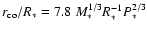 for a typical 8-day stellar period P*, which provides
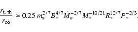 |
(7) |
Remarkably, taking typical values for CTTS with a low magnetic dipole
field gives a theoretical truncation radius not only smaller than the
co-rotation radius but also consistent with observations of inner disc
holes (Najita et al. 2003). This is in strong contrast with unobserved large
scale kG fields usually used in the literature. This implies that the
formation of funnel flows should always spin up the star unless
(i) enough stellar field lines remain connected to the disc beyond
and/or (ii) ejection of stellar angular momentum is indeed
taking place. In the following section, 2.5D numerical MHD
simulations are used to show that the conditions in (5)
are indeed those prevailing at the disc inner edge. If this is true,
then we should recover a truncation radius located at our theoretical
estimate (6) for a low dipole field of 140 G.
We use the VAC![[*]](/icons/foot_motif.gif) code
(Tóth 1996) to solve the full set of axisymmetric dimensionless
resistive MHD equations (with the magnetic permeability
code
(Tóth 1996) to solve the full set of axisymmetric dimensionless
resistive MHD equations (with the magnetic permeability
 )
in cylindrical coordinates (r, z):
)
in cylindrical coordinates (r, z):
 |
(8) |
 |
(9) |
![\begin{displaymath}\frac{\partial\vec{B}}{\partial t} + {\bf\nabla}\cdot\left(\v...
...times\left[\eta
\left({\bf\nabla}\times \vec{B}\right)\right],
\end{displaymath}](/articles/aa/full/2008/04/aa8328-07/img71.gif) |
(10) |
 |
(11) |
where  is the plasma density,
 the
poloïdal velocity,
the
poloïdal velocity,  the total velocity,
  the magnetic field, P the thermal
pressure,
the magnetic field, P the thermal
pressure,  the magnetic resistivity,
 the current density,
 the gravity
potential created by the central star and
the gravity
potential created by the central star and
 the total
energy density. The gravity is treated as a source term in the momentum
and energy equations of VAC.
the total
energy density. The gravity is treated as a source term in the momentum
and energy equations of VAC.
Time evolution is done with a conservative second order accurate total variation diminishing Lax Friedrichs scheme with minmod
limiters applied on primitive variables, except for density where a
van Leer limiter is used instead to better resolve contact
discontinuities. Powell source terms are used to ensure the divergence
free property of the magnetic field and the code has been modified so
as to compute only the deviations from the dipolar component
(Tanaka 1994; Powell et al. 1999).
The splitting technique has three main advantages. First, it is crucial
to properly represent an initial force-free configuration numerically. Second,
since the total conserved energy contains only the energy associated
with the deviation from the dipolar field, this method improves the computation
of the thermal energy in low  regions. Third, when used in association
with the Powell method, it helps control the divergence of the magnetic field,
since only the deviation from the background field is used to calculate the divergence
and the Powell source terms. The divergence method used here gives
regions. Third, when used in association
with the Powell method, it helps control the divergence of the magnetic field,
since only the deviation from the background field is used to calculate the divergence
and the Powell source terms. The divergence method used here gives
 but simulations done with PLUTO and a constraint-transport scheme
show that our results are not strongly modified by this method (Zanni et al., in prep).
but simulations done with PLUTO and a constraint-transport scheme
show that our results are not strongly modified by this method (Zanni et al., in prep).
Boundary conditions take symmetric and asymmetric conditions for the
axis and the disc midplane, while continuous (outflow) conditions are
used at the outer edge. At the inner edge corresponding to the stellar
surface, a linear extrapolation of density and pressure is made.
After using free extrapolation for the poloidal velocity, this latter
is forced to be parallel to the total poloidal magnetic field.
The poloidal field is fixed, contrary to Romanova et al. (2002).
We use a boundary condition on the toroidal magnetic field designed by
Zanni et al. (in prep.). It allows us to derive  by forcing the magnetic surfaces to locally rotate at the stellar velocity.
In practice, the radial derivative of the toroidal field is computed from the angular momentum conservation equation where the temporal derivative giving the local acceleration is replaced by
by forcing the magnetic surfaces to locally rotate at the stellar velocity.
In practice, the radial derivative of the toroidal field is computed from the angular momentum conservation equation where the temporal derivative giving the local acceleration is replaced by
 |
(12) |
where the timescale
 is the Alfvén crossing time of one cell
  at the inner edge of the simulation box.
This allows the system to evolve without imposing any arbitrary
conditions on ,
and hence on the torques.
at the inner edge of the simulation box.
This allows the system to evolve without imposing any arbitrary
conditions on ,
and hence on the torques.
![\begin{figure}
\par\includegraphics[angle=90,width=17.6cm,clip]{8328fig1.ps} \end{figure}](/articles/aa/full/2008/04/aa8328-07/Timg89.gif) |
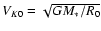
Figure 1:
Resistive MHD simulation for a 5-day period CTTS
with
 and
and
 after t=0, 5.1, 10.2, 15.3, 20.4, 25.5 Keplerian
periods at the disc inner edge corresponding to a physical
time of 1.5 months. We show the density distribution in the computational domain
using a log scale. The black lines draw the
magnetic field lines and the black arrows represent the
velocity field. The white line on the first snapshot represents an initial magnetic
field line anchored at
.
We superimpose a
part of the computational grid to show the good resolution
near the truncation radius. An accretion column is formed
between
and
(see text) and one
observes the expansion of the poloidal magnetic field and
transient disc ejecta. The accretion rate at the stellar
surface is equal to
after t=0, 5.1, 10.2, 15.3, 20.4, 25.5 Keplerian
periods at the disc inner edge corresponding to a physical
time of 1.5 months. We show the density distribution in the computational domain
using a log scale. The black lines draw the
magnetic field lines and the black arrows represent the
velocity field. The white line on the first snapshot represents an initial magnetic
field line anchored at
.
We superimpose a
part of the computational grid to show the good resolution
near the truncation radius. An accretion column is formed
between
and
(see text) and one
observes the expansion of the poloidal magnetic field and
transient disc ejecta. The accretion rate at the stellar
surface is equal to
 at t=5 and stabilises around
 at t=15.
No X-winds are formed and the star is being spun up.
at t=15.
No X-winds are formed and the star is being spun up. |
| Open with DEXTER |
In the initial conditions we take a Keplerian disc surrounded by an adiabatic corona in hydrostatic (non rotating)
equilibrium. The disc is adiabatic with an index
 and an aspect ratio
 .
The surface of the disc is determined by the pressure equilibrium between the disc and the corona, while the initial truncation
radius has been chosen arbitrarily.
The density and pressure expressions for both the disc and the corona are
.
The surface of the disc is determined by the pressure equilibrium between the disc and the corona, while the initial truncation
radius has been chosen arbitrarily.
The density and pressure expressions for both the disc and the corona are
The density contrast between the disc and the corona is
 .
A pure dipolar magnetic field is set up in the computational domain in equipartition with the thermal pressure of the disc at r=R0.
The rotation period of the star is set in order to place the corotation radius at r=2R0.
The disc has no viscosity but is resistive with an alpha-like magnetic
resistivity decreasing on a disc scale height, namely
.
A pure dipolar magnetic field is set up in the computational domain in equipartition with the thermal pressure of the disc at r=R0.
The rotation period of the star is set in order to place the corotation radius at r=2R0.
The disc has no viscosity but is resistive with an alpha-like magnetic
resistivity decreasing on a disc scale height, namely
 .
In this paper, we fix
.
The initial poloidal flow within the disc is zero and the disc is
slightly sub-Keplerian with
.
In this paper, we fix
.
The initial poloidal flow within the disc is zero and the disc is
slightly sub-Keplerian with
The grid and stellar rotation period were chosen to allow good resolution at the
truncation radius R0 while maintaining the co-rotation radius at r=2 R0 well inside the domain.
Our polar grid of
 is stretched in the
spherical R direction (see Fig. 1) and goes from
is stretched in the
spherical R direction (see Fig. 1) and goes from
 at the stellar surface to
 .
.
The results are presented in adimensional units: lengths are given in units of R0, which corresponds to the truncation
radius of the reference simulation (see Sect. 3.5); speeds are expressed in units of the
Keplerian speed
 and densities in units of
 ,
which is the initial disc density at
(r=R0, z=0).
Time is given in units of the Keplerian period at R0, i.e.
,
which is the initial disc density at
(r=R0, z=0).
Time is given in units of the Keplerian period at R0, i.e.
 .
Mass accretion rates is given in units of
.
Mass accretion rates is given in units of
 while we express the torques in units of
 .
.
We consider a
 young star with a radius of
 and a pure stellar dipole field with
.
With these assumptions the normalisation units will be
and a pure stellar dipole field with
.
With these assumptions the normalisation units will be
 ,
,
 and
and
 .
Since we place the corotation radius at 2R0, the rotation period of the star is
.
Since we place the corotation radius at 2R0, the rotation period of the star is
 days while the time will be scaled in units of
 days. The
computational domain extends up to 0.3 AU. Finally the normalisation for the accretion rates is
given by
days. The
computational domain extends up to 0.3 AU. Finally the normalisation for the accretion rates is
given by
 .
.
From these reference values, simulations done here can be scaled for
another range of parameters (R*, M*, B*) in the following way:
For these fixed stellar and accretion disc parameters, we make three simulations with different initial truncation radius
 .
Our reference simulation (s1) corresponds to an initial truncation radius fulfilling Eq. (6), namely
.
Our reference simulation (s1) corresponds to an initial truncation radius fulfilling Eq. (6), namely
 with
with
 .
Simulation (s2) is done for
.
Simulation (s2) is done for
 with
with
 and simulation (s3) for
 with
with
 .
.
We then let the system evolve and observe whether or not the real disc truncation
radius
converges towards the theoretical radius
 as given by Eq. (6). With our normalised quantities, the truncation radii in simulations (s2) and (s3) are thus expected to converge towards 1, with
 .
To check this, we identify this radius and then compute the plasma beta. It is however not straightforward to define this radius since the magnetic field is not a solid wall: the radial to vertical deviation of the flow is quite smooth. In practice, we get the truncation radius
by detecting a steep decrease in density at the disc midplane (see Fig. 4).
.
To check this, we identify this radius and then compute the plasma beta. It is however not straightforward to define this radius since the magnetic field is not a solid wall: the radial to vertical deviation of the flow is quite smooth. In practice, we get the truncation radius
by detecting a steep decrease in density at the disc midplane (see Fig. 4).
Figure 1 shows a series of snapshots of our reference simulation
(s1). The upper left panel shows the initial condition. We have
superimposed a part of the computational grid to show the resolution
achieved. We have a resolution of 8 points in the vertical direction
within the disc at each radius, while the resolution within the
accretion column reaches 20 points at the stellar surface. Magnetic
field lines are in black while the white line traces a magnetic field
line connecting the star to the co-rotation radius
 .
After a rapid transient phase with the opening of stellar field
lines, a quasi-steady situation is achieved where quasi-steady
accretion columns are formed, even with a low stellar dipole
field. The final (equilibrium) truncation radius is
.
After a rapid transient phase with the opening of stellar field
lines, a quasi-steady situation is achieved where quasi-steady
accretion columns are formed, even with a low stellar dipole
field. The final (equilibrium) truncation radius is
 ,
and thus well below the co-rotation radius.
,
and thus well below the co-rotation radius.
![\begin{figure}
\par\includegraphics[angle=90,width=8.4cm,clip]{8328fig2.ps}\end{figure}](/articles/aa/full/2008/04/aa8328-07/Timg131.gif) |
Figure 2:
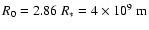
Projection of the forces in normalised units along a magnetic field line in the middle
of the accretion column, for run (s1) at t=10. We represent the gravity  ,
the centrifugal force ,
the centrifugal force
 ,
the thermal pressure gradient ,
the thermal pressure gradient  ,
the poloidal magnetic force ,
the poloidal magnetic force  and the
total force
and the
total force
 as a function of the curvilinear coordinate s. The disc midplane is located at s=0and the disc surface corresponds to
 .
Gravity begins to dominate the dynamics only at some distance between the disc and the star ( .
Gravity begins to dominate the dynamics only at some distance between the disc and the star (
 at the stellar surface).
 |
| Open with DEXTER |
Figure 2 shows the projection
 of the various forces along a magnetic field line
located at the centre of the accretion column at t=10. Since the
stellar magnetic moment is directed northwards, a negative force is
actually pulling material upwards. Accretion is achieved because of
the negative magnetic torque (not shown here) but against the poloidal
magnetic force
which tends to prevent it. Note however that it
is
negligible with respect to the other forces. What drives the poloidal
motion in the accretion column is actually the plasma pressure
gradient
which was built in by the accumulation of accreting
mass and allows it to be lifted up and loaded onto closed stellar field
lines. It acts exactly as in accretion-ejection structures, enabling
the necessary transition from the resistive MHD disc to the ideal MHD
columns (Ferreira & Pelletier 1995). The plasma pressure gradient remains dominant
well above the disc surface, located around the curvilinear
coordinate s=0.2. Given the dipole topology, this is not
surprising as material must first be lifted against gravity (
is
initially positive) by .
Then, at some point (which depends
mostly on the dipole geometry) gravity overcomes it and becomes the leading agent. Again, this is only possible because the centrifugal term
plays almost no role due to the azimuthal magnetic braking. Matter then reaches the star in a dynamical time scale with approximately free-fall velocities (
of the various forces along a magnetic field line
located at the centre of the accretion column at t=10. Since the
stellar magnetic moment is directed northwards, a negative force is
actually pulling material upwards. Accretion is achieved because of
the negative magnetic torque (not shown here) but against the poloidal
magnetic force
which tends to prevent it. Note however that it
is
negligible with respect to the other forces. What drives the poloidal
motion in the accretion column is actually the plasma pressure
gradient
which was built in by the accumulation of accreting
mass and allows it to be lifted up and loaded onto closed stellar field
lines. It acts exactly as in accretion-ejection structures, enabling
the necessary transition from the resistive MHD disc to the ideal MHD
columns (Ferreira & Pelletier 1995). The plasma pressure gradient remains dominant
well above the disc surface, located around the curvilinear
coordinate s=0.2. Given the dipole topology, this is not
surprising as material must first be lifted against gravity (
is
initially positive) by .
Then, at some point (which depends
mostly on the dipole geometry) gravity overcomes it and becomes the leading agent. Again, this is only possible because the centrifugal term
plays almost no role due to the azimuthal magnetic braking. Matter then reaches the star in a dynamical time scale with approximately free-fall velocities (
 ).
).
The strong differential rotation beyond ,
in a region where
,
leads to an expansion of the poloidal magnetic field lines. Such an expansion starts at the inner regions and enforces the outer field lines to inflate as well (but the cause there is not the differential rotation). Once these loops (inflated lines) reach the outer boundary of the computational domain, they open, mimicking a reconnection. This opening is actually an effect of the boundary conditions used but, for all practical means, we see no strong bias on the evolution of the system. Anyway, on quite short time scales ( ), most of the stellar magnetic flux not related to the accretion funnels around
has been opened (Fig. 1).
One might think that a disc wind is driven in this region of the disc as the Blandford & Payne (1982) criterion is fulfilled. Moreover, some mass is indeed leaving the disc along these open field lines. But this
is only a breeze and not a proper jet: the ejected material does not
reach super-Alfvénic speeds. We note also that no X-winds
(Shu et al. 1994) are obtained despite the favourable magnetic configuration. The reason why no disc wind is obtained, neither extended nor X-wind, is that the field threading the disc in these regions is far below equipartition.
), most of the stellar magnetic flux not related to the accretion funnels around
has been opened (Fig. 1).
One might think that a disc wind is driven in this region of the disc as the Blandford & Payne (1982) criterion is fulfilled. Moreover, some mass is indeed leaving the disc along these open field lines. But this
is only a breeze and not a proper jet: the ejected material does not
reach super-Alfvénic speeds. We note also that no X-winds
(Shu et al. 1994) are obtained despite the favourable magnetic configuration. The reason why no disc wind is obtained, neither extended nor X-wind, is that the field threading the disc in these regions is far below equipartition.
![\begin{figure}
\par\includegraphics[angle=90,width=11.5cm,clip]{8328fig3.ps}\end{figure}](/articles/aa/full/2008/04/aa8328-07/Timg135.gif) |
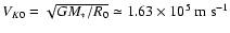
Figure 3:
Top: evolution in time of the position of the truncation
radius
(solid lines) for a set of resistive MHD simulations
with
,
P*=5.1 days and
and a different initial truncation
radius. The time unit is the Keplerian period at r=1. All runs
converge towards a truncation radius
 (solid lines). Dash-dot lines represent, for each simulation, the
radius r1 where
(solid lines). Dash-dot lines represent, for each simulation, the
radius r1 where  .
We report also the radius
(dashed line) which indicates the base of the funnel
flow,
(dashed line) and
for our reference run (s1).
Bottom: evolution in time of the sonic Mach number at the base of the funnel, .
We report also the radius
(dashed line) which indicates the base of the funnel
flow,
(dashed line) and
for our reference run (s1).
Bottom: evolution in time of the sonic Mach number at the base of the funnel,
 ,
for run (s1). ,
for run (s1). |
| Open with DEXTER |
The results of varying the initial truncation radius (simulations s2 and s3) are summarised in Fig. 3. In both cases, we observe a rapid convergence to
 on a dynamical time scale. Although some fluctuations in time can be seen in ,
it remains strikingly close to unity. Besides, it is really close to the radius of equipartition where ,
r1, with a relative position lower than 4%. This is another indication of the importance of the plasma pressure gradient in defining the truncation radius and justifies the approximation
.
on a dynamical time scale. Although some fluctuations in time can be seen in ,
it remains strikingly close to unity. Besides, it is really close to the radius of equipartition where ,
r1, with a relative position lower than 4%. This is another indication of the importance of the plasma pressure gradient in defining the truncation radius and justifies the approximation
.
The accretion rate onto the star is that which is actually
observationally determined through, e.g. veiling measurements. It is
obtained here by computing the mass flux in the accretion column,
namely
 .
Surprisingly, it is found to
converge towards
(see
Fig. 5), hence a factor 10 smaller than the mean accretion
rate in CTTS. We will come back to this issue later. If we now insert this value into Eq. (6), we find a theoretical truncation radius
.
Surprisingly, it is found to
converge towards
(see
Fig. 5), hence a factor 10 smaller than the mean accretion
rate in CTTS. We will come back to this issue later. If we now insert this value into Eq. (6), we find a theoretical truncation radius
 ,
using
,
using
 .
This is off by 20%, which is not bad considering our crude approximations of such a complicated problem.
.
This is off by 20%, which is not bad considering our crude approximations of such a complicated problem.
Since
is well verified, the main source of discrepancy in Eq. (6) is due to the assumption of
 .
This is too crude for an obvious reason. Indeed, the disc truncation radius, as measured by the steep drop in density at the equatorial plane, is actually the point where
.
This is too crude for an obvious reason. Indeed, the disc truncation radius, as measured by the steep drop in density at the equatorial plane, is actually the point where
 ,
hence
,
hence
 .
Figure 3 shows the evolution of the sonic Mach number
.
Figure 3 shows the evolution of the sonic Mach number  computed for run (s1) at
,
which corresponds to the base of the funnel flow where the poloidal magnetic pressure matches the poloidal ram pressure. It can be seen that
is larger than
by almost 30%. This is not surprising as it is necessary to first brake efficiently material (
)
before being able to lift it up (). This is also illustrated in Fig. 4 where we plot the radial profile of several quantities at the disc midplane: density ,
angular velocities (real
computed for run (s1) at
,
which corresponds to the base of the funnel flow where the poloidal magnetic pressure matches the poloidal ram pressure. It can be seen that
is larger than
by almost 30%. This is not surprising as it is necessary to first brake efficiently material (
)
before being able to lift it up (). This is also illustrated in Fig. 4 where we plot the radial profile of several quantities at the disc midplane: density ,
angular velocities (real  and Keplerian
 )
and .
Clearly, taking
to derive
is too crude. We find that using a value of
)
and .
Clearly, taking
to derive
is too crude. We find that using a value of
 ,
namely close to the real value
(see Fig. 3), provides a much better estimate with
,
namely close to the real value
(see Fig. 3), provides a much better estimate with
 close to
with an accuracy better than 10%.
close to
with an accuracy better than 10%.
![\begin{figure}
\par\includegraphics[angle=90,width=8cm,clip]{8328fig4.ps}\end{figure}](/articles/aa/full/2008/04/aa8328-07/Timg146.gif) |
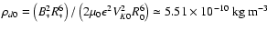
Figure 4:
Radial distributions of density ,
angular velocities
(real) and
(Keplerian) and sonic Mach number
at the disc midplane, for run (s1) after 17 Keplerian rotations. Notice the large accretion velocity in the region of opened stellar field lines. |
| Open with DEXTER |
Although the simulations here do not take into account viscosity, for
completeness, we plotted in Fig. 3 the evolution of the radius
for run (s1). To do so, we assumed
 (thus overestimating the viscous torque) and measured numerically q (see Sect. 2). As expected,
remains always significantly larger than the real truncation radius ,
which implies that criterion A is not good enough. On the other hand, criterion B would give a truncation radius located at
(thus overestimating the viscous torque) and measured numerically q (see Sect. 2). As expected,
remains always significantly larger than the real truncation radius ,
which implies that criterion A is not good enough. On the other hand, criterion B would give a truncation radius located at
 :
no accretion column should have been observed at all in our simulations. Our results clearly show that criterion B is not relevant. What about the criterion as expressed in Eq. (3)? We plotted in Fig. 3 the evolution of the radius
given by this equation and computed for run (s1). It turns out that it gives a good (though under-) estimate of the real truncation radius
as already pointed out by Romanova et al. (2002). This is because the star disc interaction introduces a sharp decrease in both the disc midplane density
and azimuthal velocity
:
no accretion column should have been observed at all in our simulations. Our results clearly show that criterion B is not relevant. What about the criterion as expressed in Eq. (3)? We plotted in Fig. 3 the evolution of the radius
given by this equation and computed for run (s1). It turns out that it gives a good (though under-) estimate of the real truncation radius
as already pointed out by Romanova et al. (2002). This is because the star disc interaction introduces a sharp decrease in both the disc midplane density
and azimuthal velocity
 (see Fig. 4). However, as stressed in Sect. 2, while basically correct, such a criterion is meaningless as a predictive tool.
As far as the formation of funnel flows is concerned, we fully confirm the results of Romanova et al. (2002): these flows are indeed robust features of axisymmetric MHD simulations. Their different boundary conditions on the magnetic field at the stellar surface, namely a fixed normal component and free conditions for  and ,
do not finally play any significant role for the truncation of the disc and the formation of accretion columns. We have also done simulations with other values of the magnetic resistivity parameter
and ,
do not finally play any significant role for the truncation of the disc and the formation of accretion columns. We have also done simulations with other values of the magnetic resistivity parameter
 with no change in the truncation radius. Note also that Romanova et al. (2002) have included viscosity in their simulations while we did not, with no significant difference in the location of the truncation radius. To be more specific, using Eq. (6) with the higher accretion rate of
 as measured by Romanova et al. (2002), we find
 for
for
 using
using
 ,
which is consistent with the truncation radius shown Fig. 16 in
Romanova et al. (2002) with a
good accuracy. Furthermore, using Eq. (6) with the values
provided by Kuker et al. (2003) one gets truncation radii smaller than the
inner radial boundary, which explains why these authors did not find
accretion columns. We are therefore confident on our main conclusion,
that is the validity of our criterion (6).
,
which is consistent with the truncation radius shown Fig. 16 in
Romanova et al. (2002) with a
good accuracy. Furthermore, using Eq. (6) with the values
provided by Kuker et al. (2003) one gets truncation radii smaller than the
inner radial boundary, which explains why these authors did not find
accretion columns. We are therefore confident on our main conclusion,
that is the validity of our criterion (6).
![\begin{figure}
\par\includegraphics[angle=90,width=8.4cm,clip]{8328fig5.ps}\end{figure}](/articles/aa/full/2008/04/aa8328-07/Timg159.gif) |
Figure 5:
Evolution in time of the accretion rate
(dash
dotted line), angular momentum flux transported by matter
 (solid line)
and by the magnetic field, computed for the closed
(solid line)
and by the magnetic field, computed for the closed
 (dash line)
and open
(dash line)
and open
 (dotted lines) field lines. The units are normalised and the two hemispheres are taken into account.
 |
| Open with DEXTER |
We now consider the fluxes of angular momentum, namely
carried in by the infalling material and
 by the magnetic field
To explicitly write these expressions we assumed that the surface element is directed inwards with respect to the surface of the star.
The flux carried by the magnetic field is the sum of that carried by
closed field lines and open field lines, namely
 .
It actually corresponds to two possible
electric circuits each related to two different electromotive
forces. A positive flux describes a positive torque acting on the star
and leading to a spin up while a negative flux leads to a spin
down. The time evolution of these fluxes is shown in
Fig. 5 for our reference run (s1). Not surprisingly, the
incoming angular momentum flux
due to the accreting
material is positive but totally negligible with respect to that
carried by the closed magnetic field lines
,
which is positive as well: the accreting star is only being spun up.
When looking more closely at
,
it turns out that there is a
negative magnetic contribution to the torque due to the open field
lines
.
This has also been previously reported in
simulations and is a natural outcome of the star-disc interaction
(Long et al. 2005). We stress however that the actual torque is not
controlled and one should not take it at face value. Indeed, this
region of the magnetosphere should be the locus of a stellar wind but
the physics of its launching has not yet been addressed.
Finally, let us turn back to our result that the accretion rate
measured onto the star is about 10 times smaller than
expected. In fact, B* and
were considered in
Eq. (6) as independent parameters. However, the mass inflow at
the inner edge of the accretion disc is constrained by the magnetic
topology. Basically, the magnetosphere acts as a nozzle and the mass
flow cannot be arbitrary. In a strict steady-state analysis it would
be imposed by the regularity condition at the slow magnetosonic
point. In our simulations, the flow reaches the slow point
.
It actually corresponds to two possible
electric circuits each related to two different electromotive
forces. A positive flux describes a positive torque acting on the star
and leading to a spin up while a negative flux leads to a spin
down. The time evolution of these fluxes is shown in
Fig. 5 for our reference run (s1). Not surprisingly, the
incoming angular momentum flux
due to the accreting
material is positive but totally negligible with respect to that
carried by the closed magnetic field lines
,
which is positive as well: the accreting star is only being spun up.
When looking more closely at
,
it turns out that there is a
negative magnetic contribution to the torque due to the open field
lines
.
This has also been previously reported in
simulations and is a natural outcome of the star-disc interaction
(Long et al. 2005). We stress however that the actual torque is not
controlled and one should not take it at face value. Indeed, this
region of the magnetosphere should be the locus of a stellar wind but
the physics of its launching has not yet been addressed.
Finally, let us turn back to our result that the accretion rate
measured onto the star is about 10 times smaller than
expected. In fact, B* and
were considered in
Eq. (6) as independent parameters. However, the mass inflow at
the inner edge of the accretion disc is constrained by the magnetic
topology. Basically, the magnetosphere acts as a nozzle and the mass
flow cannot be arbitrary. In a strict steady-state analysis it would
be imposed by the regularity condition at the slow magnetosonic
point. In our simulations, the flow reaches the slow point
 above the disc at
 (see Fig. 6). Then, it
remains supersonic with a maximum for
the sonic Mach number around
(see Fig. 6). Then, it
remains supersonic with a maximum for
the sonic Mach number around
 but the funnel flow is
always sub-Alfvénic with a maximum Alfvénic Mach number
but the funnel flow is
always sub-Alfvénic with a maximum Alfvénic Mach number
 near the middle path between the stellar surface and the disc inner edge.
![\begin{figure}
\par\includegraphics[angle=90,width=8cm,clip]{8328fig6.ps}\end{figure}](/articles/aa/full/2008/04/aa8328-07/Timg170.gif) |
Figure 6:
Sonic (dotted line), slow-magnetosonic (dashed line) and
Alfvénic (dash-dotted line) Mach numbers within the funnel flow along the same
magnetic field line at t=10 as in Fig. 2. |
| Open with DEXTER |
We have confirmed that the formation of accretion funnel flows is a robust feature of axisymmetric star-disc interactions. We investigated the physical conditions required to produce steady-state funnel flows onto a dipole and provided an analytic expression of the disc truncation radius. We then used MHD simulations with VAC to show its validity.
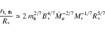
Our theoretical expression rt, th relates the disc truncation
radius to astrophysical parameters such as stellar dipole field
B*, mass M*, radius R* and accretion rate .
Although it resembles the Alfvén radius (Elsner & Lamb 1977) sometimes invoked in similar situations (Bouvier et al. 2007), it has been physically motivated on very different ground. It is shown that it gives an accurate prediction of the real truncation radius as obtained in current 2D MHD simulations of a star-disc interaction.
We report MHD simulations displaying accretion funnels with a weak stellar dipole
field
 G from a resistive non-viscous disc. In this case, the disc inner edge is found closer to the star, below the co-rotation radius, in agreement with the size of inner disc holes. However, the accretion rate onto the star which is imposed by the physics of magnetic accretion is measured to be
 .
Even though this magnitude
of accretion rate is found for some T Tauri stars
(see Gullbring et al. 1998), this result shows that it is necessary to
have stronger fields (by a factor of around 7) to have magnetospheric
accretion for typical mean accretion rates of
.
On the other hand, the few circular polarization
measurements available, provide an upper limit of 100-200 G for the
dipolar component.
However, recent spectro-polarimetric observations coupled with magnetic field
reconstruction conducted on 2 CTTS V2129 Oph and BP Tau provide
higher dipole field components of 350 G and 1.2 kG respectively
(Donati et al. 2007a, b in prep.). In any case, if the presence of kG dipole
fields around CTTS are indeed ruled out, the requirement of forming quasi-steady accretion funnels imposes that the magnetic topology must be different. This is a firm result based on our dynamical calculations.
One then needs to consider other stellar magnetic field topologies such as multipolar components and/or an inclined dipole configuration (Long et al. 2007; Romanova et al. 2003).
In this paper, since there is no viscosity on our resistive accretion
disc, we privileged a situation where
.
Even though this magnitude
of accretion rate is found for some T Tauri stars
(see Gullbring et al. 1998), this result shows that it is necessary to
have stronger fields (by a factor of around 7) to have magnetospheric
accretion for typical mean accretion rates of
.
On the other hand, the few circular polarization
measurements available, provide an upper limit of 100-200 G for the
dipolar component.
However, recent spectro-polarimetric observations coupled with magnetic field
reconstruction conducted on 2 CTTS V2129 Oph and BP Tau provide
higher dipole field components of 350 G and 1.2 kG respectively
(Donati et al. 2007a, b in prep.). In any case, if the presence of kG dipole
fields around CTTS are indeed ruled out, the requirement of forming quasi-steady accretion funnels imposes that the magnetic topology must be different. This is a firm result based on our dynamical calculations.
One then needs to consider other stellar magnetic field topologies such as multipolar components and/or an inclined dipole configuration (Long et al. 2007; Romanova et al. 2003).
In this paper, since there is no viscosity on our resistive accretion
disc, we privileged a situation where
 to reach an open magnetic topology within the main part
of the disc. This made it possible to have a braking torque feeding the disc even without viscosity. Apart from the localised magnetic flux channeling the accretion funnel, the other stellar magnetic field lines become causally disconnected from the disc.
This forbids any disc-locking mechanism and the star is being spun up
as a consequence of accretion. We also report the non development of
X-winds despite the favourable topology. Both of these aspects deserve
however a more detailed analysis as they may depend on the disc
resistivity. While the disc truncation radius remained close to its
predicted position for about 25 Keplerian periods at the disc inner
edge, some variability is obviously taking place. This is a very
promising topic as veiling measurements probing accretion onto the
star do show variability on different time scales
(Alencar & Basri 2000). However making longer simulations requires one to implement
the turbulent viscosity to allow for accretion within the disc beyond
corotation. This work is in progress.
to reach an open magnetic topology within the main part
of the disc. This made it possible to have a braking torque feeding the disc even without viscosity. Apart from the localised magnetic flux channeling the accretion funnel, the other stellar magnetic field lines become causally disconnected from the disc.
This forbids any disc-locking mechanism and the star is being spun up
as a consequence of accretion. We also report the non development of
X-winds despite the favourable topology. Both of these aspects deserve
however a more detailed analysis as they may depend on the disc
resistivity. While the disc truncation radius remained close to its
predicted position for about 25 Keplerian periods at the disc inner
edge, some variability is obviously taking place. This is a very
promising topic as veiling measurements probing accretion onto the
star do show variability on different time scales
(Alencar & Basri 2000). However making longer simulations requires one to implement
the turbulent viscosity to allow for accretion within the disc beyond
corotation. This work is in progress.
Acknowledgements
We acknowledge useful suggestions and constructive criticism of an anonymous referee on a first version of this paper.
We thank the computational facilities of the Service Commun de Calcul Intensif de l'Observatoire de Grenoble (SCCI).
The present work was supported in part by the European Community Marie Curie Actions - Human Resource and Mobility within the JETSET (Jet Simulations, Experiments and Theory) network under contract MRTN-CT-2004 005592.
- Alencar,
S. H. P., & Basri, G. 2000, AJ, 119, 119 [CrossRef], 1881
(In the text)
- Aly, J. J. 1980,
A&A, 86, 192 [NASA ADS]
- Aly, J. J., &
Kuijpers, J. 1990, A&A, 227, 473 [NASA ADS]
- Armitage, P. J.,
& Clarke, C. J. 1996, MNRAS, 280, 458 [NASA ADS]
- Arons, J. 1993, ApJ,
408, 160 [NASA ADS] [CrossRef]
- Blandford, R. D.,
& Payne, D. G. 1982, MNRAS, 199, 883 [NASA ADS]
(In the text)
- Bouvier, J., Chelli, A.,
Allain, S., et al. 1999, A&A, 349, 619 [NASA ADS]
- Bouvier, J., Grankin,
K. N., Alencar, S. H. P., et al. 2003, A&A,
409, 169 [NASA ADS] [CrossRef] [EDP Sciences]
- Bouvier, J., Alencar,
S. H. P., Harries, T. J., Johns-Krull, C. M.,
& Romanova, M. M. 2007, in Protostars and Planets V, ed.
B. Reipurth, D. Jewitt, & K. Keil, 479
- Casse, F., & Keppens, R.
2002, ApJ, 581, 988 [NASA ADS] [CrossRef]
- Cameron, A. C., & Campbell,
C. G. 1993, A&A, 274, 309 [NASA ADS]
- Donati, J.-F.,
Jardine, M. M., Gregory, S. G., et al. 2007, MNRAS, 380,
1297 [NASA ADS] [CrossRef]
(In the text)
- Edwards, S., Hartigan, P.,
Ghandour, L., & Andrulis, C. 1994, AJ, 108, 1056 [NASA ADS] [CrossRef]
- Elsner, R. F.,
& Lamb, F. K. 1977, ApJ, 215, 897 [NASA ADS] [CrossRef]
(In the text)
- Ferreira, J., &
Pelletier, G. 1995, A&A, 295, 807 [NASA ADS]
(In the text)
- Ghosh, P., & Lamb,
F. K. 1979, ApJ, 232, 259 [NASA ADS] [CrossRef]
- Gregory, S. G.,
Jardine, M., Simpson, I., & Donati, J.-F. 2006, MNRAS, 371,
999 [NASA ADS] [CrossRef]
(In the text)
- Gullbring,
E., Hartmann, L., Briceno, C., & Calvet, N. 1998, ApJ, 492,
323 [NASA ADS] [CrossRef]
(In the text)
- Hayashi,
M. R., Shibata, K., & Matsumoto, R. 1996, ApJ, 468,
L37 [NASA ADS] [CrossRef]
- Johns-Krull, C. M.,
Valenti, J. A., Hatzes, A. P., & Kanaan, A. 1999,
ApJ, 510, L41 [NASA ADS] [CrossRef]
(In the text)
- Königl, A. 1991, ApJ,
370, L39 [NASA ADS] [CrossRef]
- Küker, M., Henning,
T., & Rüdiger, G. 2003, ApJ, 589, 397 [NASA ADS] [CrossRef]
- Koldoba, A. V.,
Lovelace, R. V. E., Ustyugova, G. V., &
Romanova, M. M. 2002, AJ, 123, 2019 [NASA ADS] [CrossRef]
- Long, M., Romanova,
M. M., & Lovelace, R. V. E. 2005, ApJ, 634,
1214 [NASA ADS] [CrossRef]
- Long, M., Romanova,
M. M., & Lovelace, R. V. E. 2007, MNRAS, 374,
436 [NASA ADS] [CrossRef]
- Lovelace,
R. V. E., Romanova, M. M., & Bisnovatyi-Kogan,
G. S. 1995, MNRAS, 275, 244 [NASA ADS]
- Matt, S., & Pudritz,
R. E. 2005, MNRAS, 356, 167 [NASA ADS] [CrossRef]
- Mignone, A., Bodo,
G., Massaglia, S., et al. 2007, ApJS, 170, 228 [NASA ADS] [CrossRef]
- Miller, K. A.,
& Stone, J. M., 1997, ApJ, 489, 890 [NASA ADS] [CrossRef]
(In the text)
- Najita, J., Carr, J. S.,
& Mathieu, R. D. 2003, ApJ, 589, 931 [NASA ADS] [CrossRef]
(In the text)
- Ostriker, E. C.,
& Shu, F. H. 1995, ApJ, 447, 813 [NASA ADS] [CrossRef]
- Powell, K. G.,
Roe, P. L., Linde, T. J., Gombosi, T. I., & de
Zeeuw, D. L. 1999, J. Comp. Phys., 154, 284 [NASA ADS] [CrossRef]
- Pringle, J. E., &
Rees, M. J. 1972, A&A, 21, 1 [NASA ADS]
- Romanova, M. M.,
Ustyugova, G. V., Koldoba, A. V., & Lovelace,
R. V. E. 2002, ApJ, 578, 420 [NASA ADS] [CrossRef]
(In the text)
- Romanova, M. M.,
Ustyugova, G. V., Koldoba, A. V., Wick, J. V., &
Lovelace, R. V. E. 2003, ApJ, 595, 1009 [NASA ADS] [CrossRef]
(In the text)
- Shakura, N. I., &
Syunyaev, R. A. 1973, A&A, 24, 337 [NASA ADS]
(In the text)
- Shu, F., Najita, J.,
Ostriker, E., Wilkin, F., Ruden, S., & Lizano, S. 1994, ApJ,
429, 781 [NASA ADS] [CrossRef]
- Tanaka, T. 1994, J.
Comp. Phys., 111, 381 [NASA ADS] [CrossRef]
- Tóth, G. 1996,
Astrophys. Lett. Comm., 34, 245
(In the text)
- Ustyugova,
G. V., Koldoba, A. V., Romanova, M. M., &
Lovelace, R. V. E. 2006, ApJ, 646, 304 [NASA ADS] [CrossRef]
(In the text)
- Valenti, J. A. &
Johns-Krull, C. M. , 2004, Ap&SS, 292, 619 [NASA ADS] [CrossRef]
(In the text)
- Wang, Y. M. 1996,
ApJ, 465, 111 [NASA ADS] [CrossRef]
- Zanni, C., Ferrari, A.,
Rosner, R., Bodo, G., & Massaglia, S. 2007, A&A, 469,
811 [NASA ADS] [CrossRef] [EDP Sciences]
Copyright ESO 2008
![\begin{figure}
\par\includegraphics[angle=90,width=17.6cm,clip]{8328fig1.ps} \end{figure}](/articles/aa/full/2008/04/aa8328-07/img89.gif)
![$\displaystyle \rho_{\rm d0} \left[\frac{2}{5\epsilon^2}\left(\frac{R_0}{\sqrt{r...
...(1-\frac{5}{2}\epsilon^2\right)\frac{R_0}{r}\right)\right]^{\frac{1}{\gamma-1}}$](/articles/aa/full/2008/04/aa8328-07/img93.gif)
![\begin{figure}
\par\includegraphics[angle=90,width=8.4cm,clip]{8328fig2.ps}\end{figure}](/articles/aa/full/2008/04/aa8328-07/img131.gif)
![\begin{figure}
\par\includegraphics[angle=90,width=11.5cm,clip]{8328fig3.ps}\end{figure}](/articles/aa/full/2008/04/aa8328-07/img135.gif)
![\begin{figure}
\par\includegraphics[angle=90,width=8cm,clip]{8328fig4.ps}\end{figure}](/articles/aa/full/2008/04/aa8328-07/img146.gif)
![\begin{figure}
\par\includegraphics[angle=90,width=8.4cm,clip]{8328fig5.ps}\end{figure}](/articles/aa/full/2008/04/aa8328-07/img159.gif)
![\begin{figure}
\par\includegraphics[angle=90,width=8cm,clip]{8328fig6.ps}\end{figure}](/articles/aa/full/2008/04/aa8328-07/img170.gif)