A&A 476, 1151-1160 (2007)
DOI: 10.1051/0004-6361:20077962
A synchrotron self-Compton model with low-energy electron cut-off for the blazar S5 0716+714
O. Tsang - J. G. Kirk
Max-Planck-Institut-für Kernphysik, Saupfercheckweg 1,
69117 Heidelberg, Germany
Received 28 May 2007 / Accepted 6 September 2007
Abstract
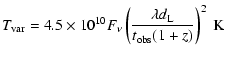
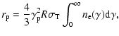
Context. In a self-absorbed synchrotron source with power-law electrons, rapid inverse Compton cooling sets in when the brightness temperature of the source reaches
 K. However, brightness temperatures inferred from observations of intra-day variable sources (IDV) are well above the "Compton catastrophe'' limit. This can be understood if the underlying electron distribution cuts off at low energy.
Aims. We examine the compatibility of the synchrotron and inverse Compton emission of an electron distribution with low-energy cut-off with that of IDV sources, using the observed spectral energy distribution of S5 0716+714 as an example.
Methods. We compute the synchrotron self-Compton (SSC) spectrum of monoenergetic electrons and compare it to the observed spectral energy distribution (SED) of S5 0716+714. The hard radio spectrum is well-fitted by this model, and the optical data can be accommodated by a power-law extension to the electron spectrum. We therefore examine the scenario of an injection of electrons, which is a double power law in energy, with a hard low-energy component that does not contribute to the synchrotron opacity.
Results. We show that the double power-law injection model is in good agreement with the observed SED of S5 0716+714. For intrinsic variability, we find that a Doppler factor of
 can explain the observed SED provided that low-frequency (<32 GHz) emission originates from a larger region than the higher-frequency emission. To fit the entire spectrum,
 is needed. We find the constraint imposed by induced Compton scattering at high
  is insignificant in our model.
Conclusions. We confirm that electron distribution with a low-energy cut-off can explain the high brightness temperature in compact radio sources. We show that synchrotron spectrum from such distributions naturally accounts for the observed hard radio continuum with a softer optical component, without the need for an inhomogeneous source. The required low energy electron distribution is compatible with a relativistic Maxwellian.
Key words: galaxies: active - galaxies: high-redshift - galaxies:
jets - BL Lacertae objects: individual: S5 0716+714
1 Introduction
Observations of many extra-galactic radio sources have found rapid
flux variations at radio frequency
(e.g. Kedziora-Chudczer et al. 2001), some of which fluctuate over a
time scale of a day or less. They are referred to as intra-day variable
sources (IDV). The variability time scale is often used to constrain
the size of the source based on causality arguments. Using this
constraint, one can derive a variability brightness temperature
(Wagner & Witzel 1995)
 |
|
|
(1) |
where the flux density  ,
wavelength
,
wavelength  ,
luminosity distant
,
luminosity distant  ,
and
observed variability time scale
,
and
observed variability time scale
 are measured in Jy, cm,
Mpc, and days, respectively.
are measured in Jy, cm,
Mpc, and days, respectively.
The high radio flux frequently measured in IDV sources implies
an extremely high brightness temperature, often many orders of magnitude
above 1012 K. Kellermann & Pauliny-Toth (1969) have shown that,
assuming the electron distribution follows a single power law, the
luminosity of the inverse Compton scattered photons exceeds that of
the synchrotron photons when the brightness temperature of the source
reaches  1012 K. Above this threshold, rapid cooling of the
relativistic electrons due to inverse Compton scattering - the "Compton
catastrophe'' - forbids a further increase in the brightness temperature
(see e.g. Kellermann 2002, for a recent review of the brightness temperature
problem). The limiting value is even lower,
1012 K. Above this threshold, rapid cooling of the
relativistic electrons due to inverse Compton scattering - the "Compton
catastrophe'' - forbids a further increase in the brightness temperature
(see e.g. Kellermann 2002, for a recent review of the brightness temperature
problem). The limiting value is even lower,
 K, if the magnetic field and particle energy density of
the source is driven towards equipartition (Readhead 1994). The
observed variability in some sources can be interpreted as the result of
extrinsic effects, which, at first sight, relaxes the size constraint.
For example, the flux variations of PKS 1519-273
and PKS 0405-385 are convincingly identified as interstellar
scintillation. Nevertheless, all realistic models of the scintillation
mechanism impose a new constraint on the size and require a brightness
temperature of
K, if the magnetic field and particle energy density of
the source is driven towards equipartition (Readhead 1994). The
observed variability in some sources can be interpreted as the result of
extrinsic effects, which, at first sight, relaxes the size constraint.
For example, the flux variations of PKS 1519-273
and PKS 0405-385 are convincingly identified as interstellar
scintillation. Nevertheless, all realistic models of the scintillation
mechanism impose a new constraint on the size and require a brightness
temperature of
 K in some cases (Macquart et al. 2000; Rickett et al. 2002),
far exceeding the limit imposed by the Compton catastrophe.
K in some cases (Macquart et al. 2000; Rickett et al. 2002),
far exceeding the limit imposed by the Compton catastrophe.
A prevalent feature associated with IDV sources is a flat or inverted
spectrum (
 ,
with flux
,
with flux
 )
at
radio-millimeter wavelengths
(e.g., Kedziora-Chudczer et al. 2001; Gear et al. 1994). Optically thick
synchrotron emission from power-law electrons rises as
)
at
radio-millimeter wavelengths
(e.g., Kedziora-Chudczer et al. 2001; Gear et al. 1994). Optically thick
synchrotron emission from power-law electrons rises as  ,
too fast to account for the observed spectra. Optically thin
synchrotron emission in the scope of the conventional interpretation
of the synchrotron theory has a flux
,
too fast to account for the observed spectra. Optically thin
synchrotron emission in the scope of the conventional interpretation
of the synchrotron theory has a flux
 ,
where s is the power-law index of the electrons
(
,
where s is the power-law index of the electrons
(
 ). If
). If
 ,
the number density of electrons diverges
towards high
,
the number density of electrons diverges
towards high  .
Imposing a high-energy cut-off in the electron
spectrum avoids the divergence and may account for the commonly
observed spectral steepening at optical frequencies, but
Marscher (1977) showed that electron spectra with
.
Imposing a high-energy cut-off in the electron
spectrum avoids the divergence and may account for the commonly
observed spectral steepening at optical frequencies, but
Marscher (1977) showed that electron spectra with  would
result in a high flux between infrared and optical frequencies that is
not supported by observations. The most common interpretation of the
flat or inverted spectra is, therefore, a superposition of many
synchrotron spectra within an inhomogeneous source
(e.g. Blandford & Konigl 1979; de Bruyn 1976; Marscher 1977).
would
result in a high flux between infrared and optical frequencies that is
not supported by observations. The most common interpretation of the
flat or inverted spectra is, therefore, a superposition of many
synchrotron spectra within an inhomogeneous source
(e.g. Blandford & Konigl 1979; de Bruyn 1976; Marscher 1977).
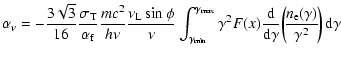
In Kirk & Tsang (2006), we discussed a synchrotron self-Compton model in
which the electron distribution is monoenergetic. The lack of low-energy electrons enables more GHz photons to emerge from the source,
allowing a higher brightness temperature to be observed without
initiating catastrophic cooling. We found that a temperature of up to
 K at GHz frequencies is possible with only a
moderate Doppler boosting factor of 10. In Tsang & Kirk (2007),
we discussed the parameters of the monoenergetic model and showed
that the assumption of equipartition of energy in the source does not prevent the
Compton catastrophe. We also showed that an injection of highly
relativistic electrons or strong acceleration in the source cannot
produce temperatures much higher than our limit due to copious
electron-positron pair production.
K at GHz frequencies is possible with only a
moderate Doppler boosting factor of 10. In Tsang & Kirk (2007),
we discussed the parameters of the monoenergetic model and showed
that the assumption of equipartition of energy in the source does not prevent the
Compton catastrophe. We also showed that an injection of highly
relativistic electrons or strong acceleration in the source cannot
produce temperatures much higher than our limit due to copious
electron-positron pair production.
In this paper, we examine the spectral properties of synchrotron
emission from monoenergetic electrons and from an electron
distribution that is a double power law in energy, by comparing the
model spectra with the observations of S5 0716+714, a BL Lac object that is one of the brightest known IDV sources, as well as a gamma-ray blazar (Hartman et al. 1999).
In doing so, we assume that the dominant targets for inverse Compton scattering
are produced within the source (SSC model).
The emission from gamma-ray blazars can also be interpreted in the context of models in which
the target photons are created externally (EC model), for example in the broad line region,
the accretion disk, or a molecular torus (Sokolov & Marscher 2005).
However, in many sources there is no observational evidence of a significant external
photon source. This is the case for S5 0716+714, where, despite much effort over the past three decades, no emission lines have been detected (e.g., Bychkova et al. 2006). Furthermore, XMM-Newton
observations of S5 0716+714 in 2004 analysed by Ferrero et al. (2006) and Foschini et al. (2006) show two spectral components in the 0.5-10 keV band, whose variability properties appear to favour the SSC interpretation. The recent extensive simultaneous observations of this object from radio to optical frequencies by Ostorero et al. (2006), together with INTEGRAL pointings at GeV -ray energies during the same period, provide the best test for our model.
In the following, we present the computation of the
stationary electron distribution and the resulting synchrotron and
inverse Compton spectra. The model spectra computed using the
monoenergetic electron approximation, as described in
Tsang & Kirk (2007), are presented first. Although adequate for the radio emission,
the monoenergetic model cannot reproduce the entire spectrum
of S5 0716+714. We therefore investigate an electron distribution that is
a double power law in energy - a hard low-energy part that
softens to a high-energy tail above a characteristic energy. In this way, the
inverted optically thin radio emission is retained and complemented by
nonthermal synchrotron emission from the high energy tail. In Sect. 2, we briefly describe these injection models. The resulting stationary
electron distribution is calculated in Sect. 3
and used for the computation of the synchrotron and inverse
Compton spectra. In Sect. 4, we compare the predictions
of these models with the observed spectral energy distribution (SED)
of the source to S5 0716+714. Our findings and some limitations of our approach are
discussed in Sect. 5 and our conclusions presented in Sect. 6.
2 The model
The homogeneous monoenergetic model discussed previously
(Kirk & Tsang 2006; Tsang & Kirk 2007) can be completely characterised by
the Doppler boosting factor

![$1/[\Gamma(1-\beta\cos\vartheta)]$](/articles/aa/full/2007/48/aa7962-07/img34.gif) (
( is the
source speed with respect to the rest frame of the host galaxy,
is the
source speed with respect to the rest frame of the host galaxy,
 the angle between the velocity and the line of sight,
and
the angle between the velocity and the line of sight,
and
 ),
the redshift of the host galaxy z, and four source parameters, the
electron number density
),
the redshift of the host galaxy z, and four source parameters, the
electron number density  ,
the magnetic field strength B, the
linear size of the source R, and the electron Lorentz factor measured in
the rest frame of the source .
For the purpose of comparison with observations, these can
be transformed into a different set of parameters. Details of the
transformation can be found in Kirk & Tsang (2006), in which ,
B, and
are replaced by the characteristic frequency of
synchrotron emission,
,
the magnetic field strength B, the
linear size of the source R, and the electron Lorentz factor measured in
the rest frame of the source .
For the purpose of comparison with observations, these can
be transformed into a different set of parameters. Details of the
transformation can be found in Kirk & Tsang (2006), in which ,
B, and
are replaced by the characteristic frequency of
synchrotron emission,
 ,
where
,
where
 ,
the Comptonisation parameter
,
the Comptonisation parameter  ,
which is the ratio of the luminosity of each successive generation of inverse Compton scattered photons to the luminosity of the previous
generation:
,
which is the ratio of the luminosity of each successive generation of inverse Compton scattered photons to the luminosity of the previous
generation:
 ,
(where
,
(where
 is
the Thomson optical depth), and the optical depth
is
the Thomson optical depth), and the optical depth
 to
synchrotron self-absorption at the observing frequency. The size of
the source, R, can be constrained, for example, by applying
causality arguments to the variation time,
to
synchrotron self-absorption at the observing frequency. The size of
the source, R, can be constrained, for example, by applying
causality arguments to the variation time,  ,
of the source:
,
of the source:
 .
.
We present in Sect. 4 the model spectra from monoenergetic
electrons that show good agreement with the observations of
S5 0716+714 at radio frequencies. The optical data can be fitted by
this model if a high-energy power-law "tail'' is added.
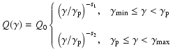
To do this, we consider an injection spectrum of the form
 for
for
 ,
where the power-law index s equals
s1 for
,
where the power-law index s equals
s1 for
 ,
and s2 for
,
and s2 for
 (Fig. 1). The electron number density at a given time is proportional to
 for s<1,
 for s>1, and
 for
s=1. In the high-energy branch of the injection spectrum, for
,
we require that s2>1, so that electron number density
congregates towards
for
s=1. In the high-energy branch of the injection spectrum, for
,
we require that s2>1, so that electron number density
congregates towards
 .
In the low-energy branch,
,
the electrons congregate at
if
s1<1. But we also require that the opacity to synchrotron
self-absorption is dominated by electrons with
.
In the low-energy branch,
,
the electrons congregate at
if
s1<1. But we also require that the opacity to synchrotron
self-absorption is dominated by electrons with
 ,
which
is achieved by demanding s1<1/3. Under the conditions s1<1/3 and
s2>1, the low-frequency synchrotron spectrum is well-approximated
by that of monoenergetic electrons with Lorentz factor
.
,
which
is achieved by demanding s1<1/3. Under the conditions s1<1/3 and
s2>1, the low-frequency synchrotron spectrum is well-approximated
by that of monoenergetic electrons with Lorentz factor
.
The electron injection spectrum cuts off at
 towards low
energy and at
towards low
energy and at
 towards high energy. The exact value of
is unimportant, since, as explained above,
synchrotron emission and opacity are dominated by electrons with
in the low-energy part of the injection
spectrum, where
determines the high frequency cut-off in the
synchrotron spectrum, at
towards high energy. The exact value of
is unimportant, since, as explained above,
synchrotron emission and opacity are dominated by electrons with
in the low-energy part of the injection
spectrum, where
determines the high frequency cut-off in the
synchrotron spectrum, at
 ,
and the highest
photon energy achievable through inverse Compton scattering in the
Klein-Nishina limit, which equals
,
and the highest
photon energy achievable through inverse Compton scattering in the
Klein-Nishina limit, which equals
 .
.
To summarise, the injection spectrum has the form
 |
|
|
(2) |
where Q0 is the electron injection rate per unit volume per unit
at
.
![\begin{figure}
\par\includegraphics[width=8cm,clip]{7962F1.eps}\end{figure}](/articles/aa/full/2007/48/aa7962-07/Timg59.gif) |
Figure 1:
Schematic representation of the electron injection spectrum and the stationary differential number density as a function of .
The heights of the spectra have been adjusted for easy comparison and are not to scale. The solid line shows the double power-law injection spectrum with power-law index s1 for
,
and s2 for
.
The dashed line shows the case where
 .
The differential electron number density .
The differential electron number density
 in regions A and B,
 in region C, and
 in region D. The dotted line shows the case where
 ,
with
in region A, ,
with
in region A,
 in region B, and
in regions C and D.
in region B, and
in regions C and D. |
| Open with DEXTER |
3 Stationary solution
The shape of the synchrotron spectrum is determined by the
stationary electron-energy distribution. Electrons injected
into the source according to Eq. (2) are
subject to radiative cooling while in the source and evacuate
this zone on a time-scale close to the light crossing time,
 .
The evolution of the electron spectrum is
governed by the kinetic equation (Kardashev 1962):
.
The evolution of the electron spectrum is
governed by the kinetic equation (Kardashev 1962):
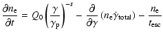 |
|
|
(3) |
where, for simplicity, we denote the differential
electron number density
 by
by  .
The second term on the right hand side of Eq. (3) is the rate of change of
the electron Lorentz factor due to radiative losses. This term is the sum of
the rates for synchrotron losses and for losses from inverse Compton scattering:
.
The second term on the right hand side of Eq. (3) is the rate of change of
the electron Lorentz factor due to radiative losses. This term is the sum of
the rates for synchrotron losses and for losses from inverse Compton scattering:
 |
|
|
(4) |
where
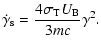 |
|
|
(5) |
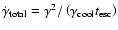
The third term is the rate at which electrons escape from the source.
In the stationary state, Eq. (3) can be solved analytically:
 |
|
|
(6) |
with the integrating factor
![$\displaystyle %
f_{\rm I}(\gamma)=
\dot{\gamma}~{\rm exp}\left[-\int^{\gamma}
\left(\dot{\gamma'}_{\rm total}t_{\rm esc}\right)^{-1}{\rm d}\gamma'\right].$](/articles/aa/full/2007/48/aa7962-07/img67.gif) |
|
|
(7) |
However, Eq. (3) is only a rough description of a source, for example,
because of the crude treatment of particle escape involved in setting
 .
Therefore, rather than use Eq. (6), we choose to use an approximate
solution that more clearly demonstrates the effects
that cooling and the evacuation of electrons from the emission
region have on the electron energy distribution.
.
Therefore, rather than use Eq. (6), we choose to use an approximate
solution that more clearly demonstrates the effects
that cooling and the evacuation of electrons from the emission
region have on the electron energy distribution.
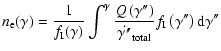
We first identify the Lorentz factor,
 ,
which determines the electron
energy at which radiative cooling dominates losses due to
particles escaping the emission region:
,
which determines the electron
energy at which radiative cooling dominates losses due to
particles escaping the emission region:
 |
|
|
(8) |
In principle,
can be evaluated only if the entire electron distribution is
already known, since
 depends on the spectrum and intensity of
emitted radiation. However, in practise, a simple iterative scheme enables it to
be found rapidly in all the cases we have computed.
Assuming it is known, solutions of Eq. (3) that are valid in the limits
depends on the spectrum and intensity of
emitted radiation. However, in practise, a simple iterative scheme enables it to
be found rapidly in all the cases we have computed.
Assuming it is known, solutions of Eq. (3) that are valid in the limits
 and
and
 are easily found.
In the first case, cooling is unimportant, and it immediately follows that
are easily found.
In the first case, cooling is unimportant, and it immediately follows that
 |
|
|
(9) |
In the second, escape is unimportant, and
the appropriate solution is found by integrating the kinetic equation once:
 |
|
|
(10) |
These solutions intersect close to the point
 .
Our approximation consists in adopting the solution without cooling
given in Eq. (9) for all Lorentz factors below the intersection point and
the solution without escape given in Eq. (10) for all Lorentz factors above the
intersection point.
.
Our approximation consists in adopting the solution without cooling
given in Eq. (9) for all Lorentz factors below the intersection point and
the solution without escape given in Eq. (10) for all Lorentz factors above the
intersection point.
In addition, we assume and verify a posteriori (see Sect. 5)
that
can be approximated by the expression for inverse Compton scattering of the synchrotron photons in the Thomson regime:
 |
|
|
(11) |
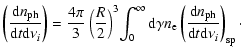
where  is the energy density of synchrotron photons in the source.
In this case,
is the energy density of synchrotron photons in the source.
In this case,
 ,
and our approximate solution is
,
and our approximate solution is
 |
|
|
(12) |
where a (1) is determined by requiring the solution (but not its first derivative)
to be continuous.
The Lorentz factors
and
give rise to breaks in ,
which
correspond to the breaks in the synchrotron spectrum at
 and
and
 .
Notice that, if s<1 (as in the injection spectrum below
),
is approximately proportional to
.
Notice that, if s<1 (as in the injection spectrum below
),
is approximately proportional to
 ,
whereas if s>1 (as in the injection spectrum above
),
is approximately
,
whereas if s>1 (as in the injection spectrum above
),
is approximately 
 .
.
Two types of stationary spectra result from Eq. (12), depending on whether the peak of the injection spectrum,
,
is below or above
.
Figure 1 shows the injection spectrum as a solid line, the stationary spectra where
 as a dotted line and where
 as a dashed line. When electrons are predominantly removed from a certain energy range by leaving the source (
 ), the spectrum retains its original shape,
 ,
since
,
since
 is independent of particle energy. On the other hand, when synchrotron losses dominates, such that
 ,
the stationary solution is
for
,
and
,
the stationary solution is
for
,
and
 for
.
For the computation of the low frequency synchrotron emission, the distribution can be approximated by a monoenergetic one at
in the first case and
in the second.
for
.
For the computation of the low frequency synchrotron emission, the distribution can be approximated by a monoenergetic one at
in the first case and
in the second.
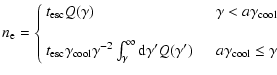
The iterative procedure used to find
is as follows: the loss rate is defined as
 |
|
|
(13) |
Then, starting with  ,
is evaluated from Eq. (8) and, using
the electron distribution given by (12),
is evaluated as described
in Sect. 3.1. The value of
,
is evaluated from Eq. (8) and, using
the electron distribution given by (12),
is evaluated as described
in Sect. 3.1. The value of  is readjusted to
 and the cycle repeated until successive values differ
by less than 1%. In the examples discussed in this paper, convergence was achieved
after two iterations. Because the change in
between iterations was
only roughly a factor of 2, the final emission spectrum was close to that found
using .
and the cycle repeated until successive values differ
by less than 1%. In the examples discussed in this paper, convergence was achieved
after two iterations. Because the change in
between iterations was
only roughly a factor of 2, the final emission spectrum was close to that found
using .
3.1 Synchrotron and inverse Compton emission
The synchrotron specific intensity, following straightforwardly from
the radiative transport equation, is
![$\displaystyle %
I_\nu^{\rm (S)}=S_\nu\left[1-{\rm exp}(-\tau_{\rm s})\right]$](/articles/aa/full/2007/48/aa7962-07/img97.gif) |
|
|
(14) |
where the optical depth to synchrotron radiation is

 ,
and
,
and
 is the absorption
coefficient (e.g., Longair 1992, Chap. 18)
is the absorption
coefficient (e.g., Longair 1992, Chap. 18)
 |
|
|
(15) |
where
 is the fine structure constant,
  the angle between the magnetic field and the direction of the emitted radiation,
 ,
,
 ,
and K5/3 is the modified Bessel function of order 5/3. The source function
,
and K5/3 is the modified Bessel function of order 5/3. The source function  is
is
 |
|
|
(16) |
In the monoenergetic approximation, the source function simplifies to
 |
|
|
(17) |
Equation (14) is integrated over frequency and angle to give
the energy density of synchrotron photons in the source
 |
|
|
(18) |
where  is a geometrical factor that is shown in Tsang & Kirk (2007) to be
  .
.
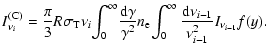
The synchrotron photons are repeatedly scattered by the energetic electrons to higher energies. Denoting by i the number of times a photon is scattered, the rate of scattering the
 generation of photons into the frequency interval
 by a single electron (see e.g., Georganopoulos et al. 2001, Eq. (4)) is
 |
|
|
(19) |
where
 |
|
|
(20) |
is the number density of the target photons, and
 the specific intensity of the
 generation of photons. The first generation of scattered photons is produced directly from the synchrotron photons: i=1,
 .
Rybicki & Lightman (1979, Chap. 7) assumed that scattering in the Thomson regime is isotropic in the rest frame of the electron, and obtained
.
Rybicki & Lightman (1979, Chap. 7) assumed that scattering in the Thomson regime is isotropic in the rest frame of the electron, and obtained
 .
Here, we include the Klein-Nishina effects (e.g., Georganopoulos et al. 2001), in which case
.
Here, we include the Klein-Nishina effects (e.g., Georganopoulos et al. 2001), in which case
| |
|
![$\displaystyle f(y) = \left[2~y~{\rm ln}~y+y+1-2y^2+{(4\epsilon_{i-1}\gamma~
y)^2(1-y)\over2(1+4\epsilon_{i-1}\gamma~ y)}\right]
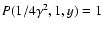
P(1/4\gamma^2,1,y),$](/articles/aa/full/2007/48/aa7962-07/img120.gif) |
(21) |
| |
|
 |
(22) |
where
 and
and
 are the energy of the target photons and scattered photon, respectively, in units of mc2, and
 for
for
 ,
and zero otherwise.
,
and zero otherwise.
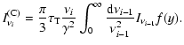
Assuming a spherical source, the rate of scattering photons with energy
 to energy
  ,
in the observer's frame, from a homogeneous distribution of electrons with differential number density
can be found by integrating over the electron energy distribution,
,
in the observer's frame, from a homogeneous distribution of electrons with differential number density
can be found by integrating over the electron energy distribution,
 |
|
|
(23) |
Note that R (the linear size of the source) is divided by 2 to obtain the source radius.
The specific intensity of the  generation photons is then the scattering rate of the electron distribution in Eq. (23) integrated over all target photon frequency,
and for a general electron distribution ,
it can be written as
 |
|
|
(25) |
For a monoenergetic electron distribution, Eq. (25) can be simplified to
 |
|
|
(26) |
Equations (26) and (25) are integrated numerically for monoenergetic electrons and for an electron distribution given by Eq. (12).
Table 1:
Model parameters corresponding to Figs. 2 and 3.
4 The BL Lac object S5 0716+714
Observations of S5 0716+714 have shown that the source exhibits intra-day variability in the radio and optical bands (e.g. Raiteri et al. 2003; Ghisellini et al. 1997). Correlation between radio (at 5 GHz) and optical (at 650 nm) variability suggest that scintillation, a process that is not effective at high radio and
optical frequencies, does not play a large part in the observed variability (Wagner 2001; Quirrenbach et al. 1991). More recent multi-frequency studies of S5 0716+714 (e.g. Agudo et al. 2006; Ostorero et al. 2006) have obtained simultaneous measurements from radio to optical frequencies during the INTEGRAL pointing period, and the non-detection of the source by INTEGRAL has provided upper limits at X-ray frequencies. Flux variations were detected at 32 and 37 GHz over a period of
 days (in November 2003) when the two-frequency measurements overlap. Since interstellar scintillation is ineffective at these frequencies, Ostorero et al. (2006) conclude that the variability is intrinsic. Assuming
 ,
with
,
with
 ,
,
 ,
and
,
and
 ,
and a redshift z>0.3 based on the non-detection of a host galaxy (e.g. Wagner et al. 1996), they derive a variability brightness temperature of
,
and a redshift z>0.3 based on the non-detection of a host galaxy (e.g. Wagner et al. 1996), they derive a variability brightness temperature of
 1014 K.
Bach et al. (2005) analysed the data set of VLBI images of 11 jet
components of S5 0716+714 at 4.9 GHz, 8.4 GHz, 15.3 GHz, and 22.2 GHz,
observed between 1992 and 2001. Assuming that all the jet components
move with the same speed along the jet (i.e. all components have the
same bulk Lorentz factor), they propose that the observed wide range
(from 5.5c to 16.1c) of apparent component speeds is due to
variations in the viewing angle and limit the Lorentz factor and the
viewing angle of the VLBI jet to  and
and
 ,
respectively. Under these conditions, the range of Doppler factors would be
,
respectively. Under these conditions, the range of Doppler factors would be
 .
.
According to Ostorero et al. (2006), observations of S5 0716+714
between 5 GHz and 32 GHz can be fitted with spectral indices
 of -0.3 and -0.5 at two different epochs. They suggest that the radio observations can be interpreted as optically thick synchrotron emission from an inhomogeneous source, and the
spectral break at
of -0.3 and -0.5 at two different epochs. They suggest that the radio observations can be interpreted as optically thick synchrotron emission from an inhomogeneous source, and the
spectral break at
 Hz would correspond to the
self-absorption frequency
Hz would correspond to the
self-absorption frequency
 .
In the near-infrared to optical
band, observations from 2001-2004, reported by
Hagen-Thorn et al. (2006) suggest that the spectral energy
distribution between the frequencies
.
In the near-infrared to optical
band, observations from 2001-2004, reported by
Hagen-Thorn et al. (2006) suggest that the spectral energy
distribution between the frequencies
 1014 Hz and
 1014 Hz can be fitted by the power law
 .
.
Here, we apply the two homogeneous models described in Sect. 2: the monoenergetic one, which successfully models the hard radio spectrum with relatively few free parameters, and
the one with double power-law injection (and, consequently more free parameters), which also enables the high-energy emission to be modelled. We adopt a value of z=0.3 for the red-shift of S5 0716+714, and a linear size inferred by the variability time scale of
days, so that
 .
The values we find for the free parameters of the models
and for several parameters derived from these are given in Table 1. The spectra predicted by the two models are shown in Figs. 2 and 3, and are discussed separately in the next two sections.
.
The values we find for the free parameters of the models
and for several parameters derived from these are given in Table 1. The spectra predicted by the two models are shown in Figs. 2 and 3, and are discussed separately in the next two sections.
Identifying the creation of our homogeneous source with an event that leads to the ejection of an individual blob observed with VLBI, we estimate the minimum jet power implied by each set of parameters by multiplying the total energy content of the source by the average rate at which blobs are ejected from the core. In the co-moving frame of the source, for monoenergetic electrons, the total energy content is
 |
|
|
(27) |
and, for power-law electrons,
 |
|
|
(28) |
Transforming to the rest frame of the galaxy,
 ,
so
that the jet power
,
so
that the jet power
 |
|
|
(29) |
where
 is the average time difference between the ejection of successive blobs. Linear fits of the change in the position of the 11 jet components (Bach et al. 2005) suggest that a new component is ejected from the core every 0.1-1.8 years. The lower limits to the jet power of each model given in Table 1 were computed using
 years.
![\begin{figure}
\par\includegraphics[width=8cm,clip]{7962F2.eps}\end{figure}](/articles/aa/full/2007/48/aa7962-07/Timg199.gif) |
Figure 2:
Spectral energy distribution of S5 0716 +714. Multi-frequency simultaneous data from Ostorero et al. (2006)
are shown as black symbols. Black dots show data points, variation
ranges are shown by a vertical bar between two symbols, and downward
arrows show upper limits. Values of the parameters are shown in
Table 1. The model spectra are computed from a
distribution of monoenergetic electrons and are shown with solid
and dashed lines. The dashed line shows the strong-magnetic-field model where
the parameters are chosen such that it goes through the data points
at optical frequency, whereas the solid line shows weak-magnetic-field model where the parameters are chosen to mimic the spectral
turning at 1011.5 Hz. The values of the parameters are shown
in Table 1. |
| Open with DEXTER |
In the monoenergetic model, the spectrum is specified by four parameters,
,
 ,
,
 ,
and ,
as well as z and
(which are kept fixed for all models). The self-absorption frequency
is determined by the first spectral break at 4 GHz, and
corresponds to
the spectral cut-off. In Fig. 2, we compare two models in which one has a cut-off at the spectral break at 1011.5 Hz, and the other cuts off just before reaching the optical point. The Doppler factor
affects the level of the observed flux both by determining the linear size of the source and determining the amount of boosting the flux receives. The Comptonisation parameter
determines the ratio of the synchrotron flux to the inverse Compton flux, as well as the value of
.
Therefore, after specifying
and
,
must be adjusted to compensate for its effect on the level of the observed flux and to ensure the inverse Compton spectra do not exceed the INTEGRAL upper limits, while minimising .
,
and ,
as well as z and
(which are kept fixed for all models). The self-absorption frequency
is determined by the first spectral break at 4 GHz, and
corresponds to
the spectral cut-off. In Fig. 2, we compare two models in which one has a cut-off at the spectral break at 1011.5 Hz, and the other cuts off just before reaching the optical point. The Doppler factor
affects the level of the observed flux both by determining the linear size of the source and determining the amount of boosting the flux receives. The Comptonisation parameter
determines the ratio of the synchrotron flux to the inverse Compton flux, as well as the value of
.
Therefore, after specifying
and
,
must be adjusted to compensate for its effect on the level of the observed flux and to ensure the inverse Compton spectra do not exceed the INTEGRAL upper limits, while minimising .
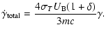
Figure 2 shows the measurements and variable ranges obtained from the simultaneous multi-frequency observation of S5 0716+714 from the study conducted by Ostorero et al. (2006). Also shown are the spectra predicted by the model assuming electrons are monoenergetic. The Doppler boosting factor is
 in both models. The weak-magnetic-field model has a synchrotron self-absorption frequency of
 GHz with a synchrotron spectrum that peaks at
 GHz (the values of other parameters are shown in Table 1). This model gives a brightness temperature of
 1012 K at
 GHz (
GHz (
 ,
where
,
where  is the Boltzmann constant and
 the angular diameter of the source). The synchrotron spectrum shows good agreement with the data points at radio frequencies. The first-order inverse-Compton spectrum gives emission from optical to soft X-ray frequencies and the second-order spectrum gives gamma-ray emission up to 40 MeV, while emission from higher orders scattering is negligible due to the Klein-Nishina effect.
The strong-magnetic-field model has
GHz, with its synchrotron peak at
 1012 Hz (the values of other parameters can be found in Table 1) and gives a brightness temperature of
 1012 K at the observing frequency
GHz. The synchrotron spectrum extends up to optical frequencies, and gives a reasonable fit at radio frequencies up to 1011.5 Hz. The first-order inverse-Compton spectrum gives X-ray emission, the second-order inverse-Compton spectrum is greatly reduced by the Klein-Nishina effects, and very little gamma-ray emission is produced.
1012 K at the observing frequency
GHz. The synchrotron spectrum extends up to optical frequencies, and gives a reasonable fit at radio frequencies up to 1011.5 Hz. The first-order inverse-Compton spectrum gives X-ray emission, the second-order inverse-Compton spectrum is greatly reduced by the Klein-Nishina effects, and very little gamma-ray emission is produced.
The spectral break at 1011.5 Hz is well-fitted by the weak-magnetic-field model. We are unable to obtain a set of parameters to allow the first inverse Compton spectrum to reproduce the optical data. Simple qualitative analysis shows that mimicking the optical data points with the first inverse Compton spectrum is inconsistent with observation. The level of flux that the first inverse-Compton spectrum would require in order to account for the optical data is much higher than the synchrotron flux (i.e.  ), so a large
would therefore be required, resulting in the spectrum extending to frequencies far beyond the optical band. The first inverse-Compton spectrum would therefore exceed the INTEGRAL upper limits, and the very high X- and -ray flux would result in copious electron-positron pair production as the -ray photons interact with the synchrotron photons.
), so a large
would therefore be required, resulting in the spectrum extending to frequencies far beyond the optical band. The first inverse-Compton spectrum would therefore exceed the INTEGRAL upper limits, and the very high X- and -ray flux would result in copious electron-positron pair production as the -ray photons interact with the synchrotron photons.
Alternatively, one can attempt to include the optical data in the synchrotron spectrum, as shown by the strong-magnetic-field model. The Lorentz factor of this model is higher than
,
which implies that the particles lose a significant portion of their energy by synchrotron radiation before they vacate the source, so the electron spectrum will evolve into one that is proportional to
 .
This set of parameters therefore violates the monoenergetic assumption. Furthermore, the predicted spectrum fails to account for the spectral break at
.
This set of parameters therefore violates the monoenergetic assumption. Furthermore, the predicted spectrum fails to account for the spectral break at
 Hz, and the optical flux is very sensitively to the electron Lorentz factor. This model is, therefore, inconsistent. It is apparent that, in order to reproduce the observed optical emission, a power-law component in the electron spectrum at
must be incorporated, which emits synchrotron radiation at a frequency above
.
Hz, and the optical flux is very sensitively to the electron Lorentz factor. This model is, therefore, inconsistent. It is apparent that, in order to reproduce the observed optical emission, a power-law component in the electron spectrum at
must be incorporated, which emits synchrotron radiation at a frequency above
.
![\begin{figure}
\par\includegraphics[width=12cm,clip]{7962F3.eps}\end{figure}](/articles/aa/full/2007/48/aa7962-07/Timg213.gif) |
Figure 3:
The spectral energy distribution of S5 0716 +714, as represented in Fig. 2. The model spectra, shown as solid and dashed lines, are computed from a quasi-monoenergetic electron distribution in the form of Eq. (12). The dashed line represents the low-Doppler-factor model where the Doppler boosting factor is minimised, whereas the solid line shows the high-Doppler-factor model where the values of the parameters are chosen to account for all radio and optical data points. The dashed gridline shows the position of 32 GHz. The values of the parameters are shown in Table 1. Historical data, as compiled by Ostorero et al. (2006) and shown as grey symbols,
at radio-to-optical frequencies are from Kuehr et al. (1981), Waltman et al. (1981), Eckart et al. (1982), Perley (1982), Perley et al. (1982), Lawrence et al. (1985), Saikia et al. (1987), Kuehr & Schmidt (1990), Moshir et al. (1990), Hales et al. (1991), Krichbaum et al. (1993), Gear et al. (1994), Hales et al. (1995), Douglas et al. (1996), Rengelink et al. (1997), Zhang et al. (1997), Riley et al. (1999), Cohen et al. (2002), Raiteri et al. (2003); UV data from Pian & Treves (1993), Ghisellini et al. (1997); X-ray data from Biermann et al. (1992), Comastri et al. (1997), Kubo et al. (1998), Giommi et al. (1999), Tagliaferri et al. (2003), Pian et al. (2005); and -ray data from McNaron-Brown et al. (1995), Hartman et al. (1999), Collmar (2006). |
| Open with DEXTER |
The Comptonisation parameter
in this model must account for the dependence of the
electron density. It is therefore redefined as
 |
|
|
(30) |
which is consistent with the definition used in the monoenergetic model.
However, for the purpose of fitting the flux in the INTEGRAL frequency
range,
1018-1020 Hz, we introduce a parameter  ,
that determines the ratio of flux between
and
,
that determines the ratio of flux between
and
 .
Inspection of the solid line
in Fig. 2 shows that synchrotron photons at the
spectral break
.
Inspection of the solid line
in Fig. 2 shows that synchrotron photons at the
spectral break
 GHz are scattered to
 Hz. Therefore,
is a
parameter that allows us to specify the spectral break
and then
to adjust the flux in the INTEGRAL frequency range. The normalisation
constant in the double power-law injection spectrum, Q0 is
eliminated in favour of the parameter
Hz. Therefore,
is a
parameter that allows us to specify the spectral break
and then
to adjust the flux in the INTEGRAL frequency range. The normalisation
constant in the double power-law injection spectrum, Q0 is
eliminated in favour of the parameter
 |
|
|
(31) |
with
 given by Eq. (12). In the monoenergetic approximation,
is equivalent to .
Therefore, using the monoenergetic model and specifying
and
,
the radio and the X-ray flux can be adjusted with
given by Eq. (12). In the monoenergetic approximation,
is equivalent to .
Therefore, using the monoenergetic model and specifying
and
,
the radio and the X-ray flux can be adjusted with
 and ,
and
and ,
and
 can be calculated.
In the low-Doppler-factor model (Figs. 3 and 4), we attempt to minimise the Doppler factor of the source. According to Wagner et al. (1996) and Ostorero et al. (2006), the variability displayed by S5 0716+714 is intrinsic, and the variation time
days was measured at 32 GHz and 37 GHz. Therefore, we require that the model spectrum must agree with the data at these two frequencies. We are unaware of correlated simultaneous variability measurement at lower frequencies during this campaign and, therefore, allow the model spectrum to deviate from the data at frequencies below 32 GHz. At the expense of having a lower flux than what is observed at frequencies below 32 GHz, we find that the minimum Doppler factor required is reduced to
 .
.
The power-law indices of the injection spectrum used to generate the spectrum of the low-Doppler-factor model are s1=-2 for the low-energy part, such that electrons with
do not contribute significantly to the synchrotron opacity, and s2=2.60, chosen for constructing the spectral shape in the infrared to optical band. The rest of the parameters are varied while keeping the Doppler boosting factor fixed. To find the limiting case, we have chosen the self absorption frequency to be
 GHz and find that the minimum Doppler factor that can generate a high enough level of flux at 32 GHz and beyond is
.
The values of the other parameters can be found in Table 1. At the observing frequency of 32 GHz, the brightness temperature in the frame of the observer is
GHz and find that the minimum Doppler factor that can generate a high enough level of flux at 32 GHz and beyond is
.
The values of the other parameters can be found in Table 1. At the observing frequency of 32 GHz, the brightness temperature in the frame of the observer is
 1013 K. The frequency at which the synchrotron
spectrum cuts off does not affect the spectral shape at low frequencies. However,
1013 K. The frequency at which the synchrotron
spectrum cuts off does not affect the spectral shape at low frequencies. However,

 is constrained by the optical data, which imposes a lower limit on
 ,
and the INTEGRAL upper limits, which impose an upper limit on
.
The maximum value is shown in this model, where
,
and the INTEGRAL upper limits, which impose an upper limit on
.
The maximum value is shown in this model, where
 Hz. This equates to
 105 with
and z=0.3.
105 with
and z=0.3.
The low-Doppler-factor model shows that it is possible to interpret the observed variability at 32 GHz and 37 GHz as coming from one of the jet components with the kinematics
described by Bach et al. (2005). That would require the lower-frequency emission to originates from a larger region than what is inferred from the observed variability at  GHz.
GHz.
In the high-Doppler-factor model (Figs. 3 and 4) we assume the emission at all frequencies - including the low frequency (<32 GHz) radio - originates from a single homogeneous source. This is suggested by the correlation between the variability at 5 GHz and 650 nm observed in February 1990 (Wagner et al. 1996; Quirrenbach et al. 1991). The parameter
must be kept small, so that the inverse Compton spectra are below the INTEGRAL upper limits. This is achieved at the expense of a relatively high Doppler factor, at
 .
The brightness temperature at 32 GHz is
.
The brightness temperature at 32 GHz is
 1012 K. This model also shows the minimum value of
,
found to be
1012 K. This model also shows the minimum value of
,
found to be
 1015 Hz.
The high-Doppler-factor model shows that if the emission at all frequencies originate from a single source region, it must be boosted by a much higher Doppler factor than proposed for the jet components by Bach et al. (2005). Even with a viewing angle
 ,
in which case
,
in which case
 ,
a bulk Lorentz factor of
,
a bulk Lorentz factor of  is required, suggesting either that the source was travelling at a much higher speed than during the observations analysed by Bach et al. (2005) or that an interpretation of the superluminal motion in the VLBI jet that infers a much higher bulk Lorentz factor should be applied. One such suggestion is a conical jet (Gopal-Krishna et al. 2006). Alternatively, the jet components may decelerate as they travel down the jet (Marscher 1999; Ghisellini et al. 2005; Georganopoulos & Kazanas 2003). The wide range of superluminal velocities shown in Bach et al. (2005) would then be a combined result of the variations in speed, as well as of the viewing angle.
![\begin{figure}
\par\includegraphics[width=7.5cm,clip]{7962F4a.eps}\par\includegraphics[width=7.5cm,clip]{7962F4b.eps}\end{figure}](/articles/aa/full/2007/48/aa7962-07/Timg236.gif) |
Figure 4:
The spectral energy distribution of S5 0716 +714 and the model spectra, as represented in Fig. 2, in the radio-to-optical band. Top panel shows the low-Doppler-factor model where the Doppler boosting factor is minimised. Bottom panel shows the high-Doppler-factor model where the values of the parameters are chosen to account for all radio and optical data points. |
| Open with DEXTER |
5 Discussion
The spectra of the four models - two monoenergetic and two with double power-law electron injection - shown in Figs. 2 and 3, show brightness temperatures at 32 GHz that are well above the conventional Compton limit. However, due to the lack of low-energy electrons, these brightness temperatures in fact lie below the threshold of the Compton catastrophe (i.e.,  )
and are, therefore, sustainable by the source.
)
and are, therefore, sustainable by the source.
An independent limit on
is provided by induced Compton
scattering, when low-energy electrons couple with high-frequency
photons. The photon occupation number
 ,
which implies that the photon occupation
number is high at and below the peak (where
,
which implies that the photon occupation
number is high at and below the peak (where
 )
of the synchrotron spectrum. In the presence of low-energy electrons, induced Compton scattering of photons at frequency
to frequencies
)
of the synchrotron spectrum. In the presence of low-energy electrons, induced Compton scattering of photons at frequency
to frequencies
 becomes increasingly significant as the synchrotron flux
grows. Sunyaev (1971) showed that this process limits the
brightness temperature at a certain frequency to
becomes increasingly significant as the synchrotron flux
grows. Sunyaev (1971) showed that this process limits the
brightness temperature at a certain frequency to
 109 K for
 .
Sincell & Krolik (1994) demonstrated by numerical
simulations that relativistic induced Compton scattering limits the
brightness temperature of a self-absorbed synchrotron source to
.
Sincell & Krolik (1994) demonstrated by numerical
simulations that relativistic induced Compton scattering limits the
brightness temperature of a self-absorbed synchrotron source to

 K, where
 is the observing frequency in units of GHz,
is the low energy cut-off in the
electron spectrum
is the observing frequency in units of GHz,
is the low energy cut-off in the
electron spectrum
 .
For a conventional power-law
electron spectrum in which
.
For a conventional power-law
electron spectrum in which
 ,
this gives a limit of
1011 K at 1 GHz.
,
this gives a limit of
1011 K at 1 GHz.
One might suspect that, at such high brightness temperatures as are
predicted by the models shown here, the effect of induced Compton
scattering should be significant. Qualitative arguments reveal the
contrary in our model, since the low-energy cut-off in the electron
spectrum is effectively
,
and the occupation number (
 )
of photons at frequencies that would couple with
electrons at
is negligibly small. Alternatively, when using the
result of Sincell & Krolik (1994), one finds that the limit corresponds to
)
of photons at frequencies that would couple with
electrons at
is negligibly small. Alternatively, when using the
result of Sincell & Krolik (1994), one finds that the limit corresponds to

 K for
K for
 and
and
 .
.
The spectral break at 1011.5 Hz was interpreted by Ostorero et al. (2006) as the result
of the change in opacity of the source. In our interpretation, the break is a result of a corresponding spectral break in the electron spectrum; below this frequency, the synchrotron spectrum remains optically thin. The self-absorption frequency
lies at a much lower frequency (4 GHz) in our model, which implies a weaker magnetic field and/or a lower electron density. This interpretation therefore does not require an inhomogeneous magnetic field and electron density.
The spectral index of the high-energy "tail'' of the synchrotron
spectrum beyond the first spectral break depends on whether
lies below or above
,
since this affects the final shape of
the electron spectrum, as explained in Sect. 3. If the number of electrons leaving the energy
 is dominated by cooling by radiation, the synchrotron spectrum continues from
 between
and
,
to
between
and
,
to
 between
and
,
then
between
and
,
then
 between
and
,
and it is cut off exponentially beyond
.
In this case, the
low radio-frequency spectrum resembles that of a monoenergetic
electron distribution of energy
between
and
,
and it is cut off exponentially beyond
.
In this case, the
low radio-frequency spectrum resembles that of a monoenergetic
electron distribution of energy
 .
If, on the other hand,
losses are dominated by electrons evacuating the emission zone on a
time scale of
,
the synchrotron spectrum then
continues from
between
and
,
to
.
If, on the other hand,
losses are dominated by electrons evacuating the emission zone on a
time scale of
,
the synchrotron spectrum then
continues from
between
and
,
to
 between
and
,
then
between
and
,
and it is again
cuts off exponentially beyond
.
The low radio-frequency synchrotron spectrum can be approximated in the same way as the one from a monoenergetic distribution of electron of energy
.
between
and
,
then
between
and
,
and it is again
cuts off exponentially beyond
.
The low radio-frequency synchrotron spectrum can be approximated in the same way as the one from a monoenergetic distribution of electron of energy
.
Observations of S5 0716+714 from infrared to optical frequencies
suggest that the spectral energy distribution between the frequencies
1014 Hz and
1014 Hz can be well-fitted by the power law
(Hagen-Thorn et al. 2006). Clearly, the top
panel in Fig. 4 is much too hard at these
frequencies. However, the spectrum can be softened by lowering the
cut-off frequency of the synchrotron spectrum
(i.e., bottom
panel in Fig. 4). By decreasing
to
approximately
 ,
the spectrum begins an exponential drop
at or just before reaching the relevant frequency range and, as a
result, softens the spectrum, without altering the level of flux or
the spectral shape at frequencies <
.
,
the spectrum begins an exponential drop
at or just before reaching the relevant frequency range and, as a
result, softens the spectrum, without altering the level of flux or
the spectral shape at frequencies <
.
![\begin{figure}
\par\includegraphics[width=7.5cm,clip]{7962F5a.eps}\par\includegraphics[width=7.5cm,clip]{7962F5b.eps}\end{figure}](/articles/aa/full/2007/48/aa7962-07/Timg261.gif) |
Figure 5:
Cooling rates normalised to the synchrotron loss rates (dashed lines at
 ). The rate for inverse Compton scattering is shown as a dotted line, the total loss rate as a thin solid line (blue online). The approximate rate used to compute the electron distribution is shown as a thick solid line (black online). The top ( bottom) panel shows the results of the low(high)-Doppler-factor model shown as dashed (solid) lines in Fig. 3. The vertical dotted lines correspond to ). The rate for inverse Compton scattering is shown as a dotted line, the total loss rate as a thin solid line (blue online). The approximate rate used to compute the electron distribution is shown as a thick solid line (black online). The top ( bottom) panel shows the results of the low(high)-Doppler-factor model shown as dashed (solid) lines in Fig. 3. The vertical dotted lines correspond to
 (see Eq. (12)) on the left, and to
 on the right.
 |
| Open with DEXTER |
Figure 2 and the bottom panel in Fig. 4
demonstrate that, if the variability of S5 0716+714 is intrinsic and
extends down to <32 GHz, the Doppler-boosting factor of the
emission region must be much higher than the 20-30 suggested by
Bach et al. (2005). One possibility for enabling the
Doppler factor to fall within this range is to increase the magnetic
field strength and the electron density, as shown in
Table 1. This causes the synchrotron self-absorption
frequency
to increase, as shown by the top panel in
Fig. 4, therefore requiring the assumption that the
emission at frequency below
originates from a larger region
than inferred from the variability at 32 GHz and
37 GHz. Requiring the value of
 GHz, we find that, to remain below the INTEGRAL upper limits, we require a minimum Doppler factor of
and a minimum self-absorption
frequency of
GHz. Below these minima, the model spectrum
would either have a level of flux below the measured flux at radio
frequencies or the subsequent first inverse Compton spectrum would
lie above the INTEGRAL upper limits.
GHz, we find that, to remain below the INTEGRAL upper limits, we require a minimum Doppler factor of
and a minimum self-absorption
frequency of
GHz. Below these minima, the model spectrum
would either have a level of flux below the measured flux at radio
frequencies or the subsequent first inverse Compton spectrum would
lie above the INTEGRAL upper limits.
The models shown here depart from the equipartition of magnetic and
particle energy, and are dominated by the energy of the relativistic
electrons (except for the rejected model). Estimating the energy
required by the source from the host galaxy,
 ,
we find
that the power required from the source by our models is
consistent with what is expected from a low-energy peaked BL Lac object
(see e.g., Nieppola et al. 2006).
,
we find
that the power required from the source by our models is
consistent with what is expected from a low-energy peaked BL Lac object
(see e.g., Nieppola et al. 2006).
An approximation inherent in our method is that, as far as their effect on the electron distribution is concerned, inverse Compton losses are dominated by single scatterings off the synchrotron photons and may be treated in the Thomson approximation. For each of the models presented in Fig. 4, we show in Fig. 5 the total rate of radiative cooling of an electron (thin solid lines, blue online) computed using the full Klein-Nishina loss rate for scattering on the full output spectrum. This should be compared with the thick solid lines (black online) that give the loss rates used in computing the electron density according to Eq. (3). These lines are horizontal and give the quantity
 for the converged model solutions. The range over which cooling is important in our approximate solution lies between the vertical lines at
and
in this figure. (In the lower panel, these lines lie close together.) The maximum deviation in this range is roughly 20% and occurs at
for the model with a relatively low Doppler factor (plotted as a dashed line in Fig. 4). The deviation for the higher Doppler factor model is less than 3%. We conclude that this approximation has a negligible effect on the electron distribution. The computation of the output spectrum from the electron distribution is not affected by this approximation, since
the full Klein-Nishina expression for the emissivity is used.
for the converged model solutions. The range over which cooling is important in our approximate solution lies between the vertical lines at
and
in this figure. (In the lower panel, these lines lie close together.) The maximum deviation in this range is roughly 20% and occurs at
for the model with a relatively low Doppler factor (plotted as a dashed line in Fig. 4). The deviation for the higher Doppler factor model is less than 3%. We conclude that this approximation has a negligible effect on the electron distribution. The computation of the output spectrum from the electron distribution is not affected by this approximation, since
the full Klein-Nishina expression for the emissivity is used.
A testable prediction of our models is correlated variability. The
hard
 radio spectral component between 30 GHz
and several hundred GHz is interpreted as the optically thin emission
of electrons whose characteristic synchrotron frequency lies at or
above hundreds of GHz. Consequently, fluctuations in the number of
such particles should be simultaneously reflected in broad-band
fluctuations of the specific intensity of radiation at these
frequencies. We are not aware of studies that investigate such an
effect.
radio spectral component between 30 GHz
and several hundred GHz is interpreted as the optically thin emission
of electrons whose characteristic synchrotron frequency lies at or
above hundreds of GHz. Consequently, fluctuations in the number of
such particles should be simultaneously reflected in broad-band
fluctuations of the specific intensity of radiation at these
frequencies. We are not aware of studies that investigate such an
effect.
The variability of the synchrotron spectrum should also be correlated
to the variability of the inverse Compton spectrum, since the same
electrons are responsible for both emissions. Analysis of XMM observation by Ferrero et al. (2006) show correlated variability between two X-ray spectral components of S5 0716+714,
which were interpreted as the high-energy part of the synchrotron spectrum and
the low-energy part of the inverse Compton spectrum. In the context of
our model, the synchrotron component is the emission from the high-energy tail of the electron spectrum, whereas the IC component is the synchrotron emission of the hard low-energy electron spectrum scattered by the same low energy electrons. The study by
Ferrero et al. (2006) therefore does not provide a direct
test of our model, although their data support an SSC interpretation.
Similarly, the polarisation properties of the 30-100 GHz
emission are predicted to be those of the single-particle synchrotron
emission. One aspect of this is the possibility that the intrinsic
circular polarisation of the source might reach a few percent
(Kirk & Tsang 2006). Another concerns the degree of linear
polarisation. Power-law electron distributions radiating in a source
with a completely homogeneous magnetic field can theoretically reach
quite high degrees of linear polarisation (up to 
 ,
depending weakly on the power-law index). These values are not reached
in extra-galactic radio sources, probably because the magnetic field
direction within the source is tangled. In general, higher degrees of
polarisation are found at higher frequency, consistent with the
conventional picture in which the source size decreases with increasing
frequency.
,
depending weakly on the power-law index). These values are not reached
in extra-galactic radio sources, probably because the magnetic field
direction within the source is tangled. In general, higher degrees of
polarisation are found at higher frequency, consistent with the
conventional picture in which the source size decreases with increasing
frequency.
In our model, however, the degree of
linear polarisation in the radio is determined by monoenergetic electrons.
According to standard synchrotron theory, this
tends to  at low frequency
(
at low frequency
(
 ), rises to
  at x=1, and tends to
  at
at  .
The effect of a tangled field within the source reduces
these values, but is independent of observing frequency. Thus, as in
conventional inhomogeneous models, the degree of linear polarisation
is predicted to increase
with frequency. However, more quantitative predictions would
require consideration of effects, such as internal Faraday rotation,
and lie outside the scope of the present paper.
.
The effect of a tangled field within the source reduces
these values, but is independent of observing frequency. Thus, as in
conventional inhomogeneous models, the degree of linear polarisation
is predicted to increase
with frequency. However, more quantitative predictions would
require consideration of effects, such as internal Faraday rotation,
and lie outside the scope of the present paper.
Finally, we note that the hard electron injection spectrum that we
have adopted (
 )
corresponds to the low-energy
(
)
corresponds to the low-energy
(
 )
part of a relativistic thermal
distribution. According to Table 1, the corresponding electron
temperature would lie at around 1012 K. In an electron-ion
plasma, this corresponds to the temperature of shocked gas behind a
mildly relativistic shock front, if one assumes that the electrons
and ions equilibrate to a
common temperature. Recent P.I.C. simulations suggest that
this assumption may indeed be justified (Spitkovsky 2007).
)
part of a relativistic thermal
distribution. According to Table 1, the corresponding electron
temperature would lie at around 1012 K. In an electron-ion
plasma, this corresponds to the temperature of shocked gas behind a
mildly relativistic shock front, if one assumes that the electrons
and ions equilibrate to a
common temperature. Recent P.I.C. simulations suggest that
this assumption may indeed be justified (Spitkovsky 2007).
6 Conclusion
Using the specific case of S5 0716+714 as an example, we confirm that it
is possible to produce high brightness temperatures at GHz frequencies
in compact radio sources without the onset of catastrophic cooling,
provided that the radiating particles have a distribution
that is sufficiently hard below a characteristic. In addition, we show qualitatively
that induced Compton scattering is insignificant in sources with a low-energy electron cut-off despite the high brightness temperature, the underlying reason being the low occupation number of the photons that can couple with the electrons at the cut-off energy.
The model where an electron distribution that is a double power law
in energy, peaking at
,
is injected into the source offers
more flexibility at higher frequencies in the synchrotron spectrum
(from infrared to optical) at the expense of more free parameters,
compared to either monoenergetic or single power-law
distributions. These parameters should be constrained by simultaneous
observations due to the highly variable nature of IDV sources. In the
case of S5 0716+714 where such data is available, the spectral break
at about 230 GHz determines the value of
,
the optical
data at 5
1014 Hz gives the lower limit of
,
as well
as constraining the spectral index s2, and the INTEGRAL upper
limits give the upper limit of
and also constrain the value
of ,
which in turn determines the electron density.
The example of S5 0716+714 illustrates several important spectral
properties of an electron distribution with a low-energy
cut-off, as described in the previous sections. The most noticeable
feature is the hard, inverted, optically thin synchrotron spectrum,
spanning a wide frequency range, which is a
prevalent feature in compact radio sources at radio frequencies
(e.g., Kedziora-Chudczer et al. 2001; Gear et al. 1994). Other features are
the spectral breaks at
,
,
and the exponential cut-off at
.
This model, therefore, allows a simple
homogeneous source to reproduce the common features shown by many IDV sources.
Acknowledgements
We thank Luisa Ostorero and Stefan Wagner for helpful discussions and
for providing us with easy access to the observational data. We would also like to thank the anonymous referee for constructive comments and suggestions that we feel have led to a significant
improvement in this paper.
- Agudo, I.,
Krichbaum, T. P., Ungerechts, H., et al. 2006, A&A,
456, 117 [NASA ADS] [CrossRef] [EDP Sciences]
- Bach, U.,
Krichbaum, T. P., Ros, E., et al. 2005, A&A, 433,
815 [NASA ADS] [CrossRef] [EDP Sciences]
(In the text)
-
Biermann, P. L., Schaaf, R., Pietsch, W., et al. 1992,
A&AS, 96, 339 [NASA ADS]
(In the text)
-
Blandford, R. D., & Konigl, A. 1979, ApJ, 232, 34 [NASA ADS] [CrossRef]
- Bychkova,
V. S., Kardashev, N. S., Boldycheva, A. V., Gnedin,
Y. N., & Maslennikov, K. L. 2006, Astron. Rep., 50,
802 [NASA ADS] [CrossRef]
(In the text)
- Cohen,
A. S., Lane, W. M., Cotton, W. D., et al. 2002,
in BAAS, 1274
(In the text)
- Collmar, W. 2006,
in Blazar Variability Workshop II: Entering the GLAST Era,
ed. H. R. Miller, K. Marshall, J. R. Webb,
& M. F. Aller, ASP Conf. Ser., 350, 120
(In the text)
-
Comastri, A., Fossati, G., Ghisellini, G., & Molendi, S. 1997,
ApJ, 480, 534 [NASA ADS] [CrossRef]
(In the text)
- de Bruyn,
A. G. 1976, A&A, 52, 439 [NASA ADS]
- Douglas,
J. N., Bash, F. N., Bozyan, F. A., Torrence,
G. W., & Wolfe, C. 1996, AJ, 111, 1945 [NASA ADS] [CrossRef]
(In the text)
- Eckart, A.,
Pauliny-Toth, I. I. K., Witzel, A., et al. 1982,
A&A, 108, 157 [NASA ADS]
(In the text)
- Ferrero,
E., Wagner, S. J., Emmanoulopoulos, D., & Ostorero, L.
2006, A&A, 457, 133 [NASA ADS] [CrossRef] [EDP Sciences]
(In the text)
-
Foschini, L., Tagliaferri, G., Pian, E., et al. 2006, A&A,
455, 871 [NASA ADS] [CrossRef] [EDP Sciences]
(In the text)
- Gear,
W. K., Stevens, J. A., Hughes, D. H., et al.
1994, MNRAS, 267, 167 [NASA ADS]
- Georganopoulos, M., &
Kazanas, D. 2003, ApJ, 594, L27 [NASA ADS] [CrossRef]
- Georganopoulos, M., Kirk,
J. G., & Mastichiadis, A. 2001, ApJ, 561, 111 [NASA ADS] [CrossRef]
(In the text)
-
Ghisellini, G., Villata, M., Raiteri, C. M., et al. 1997,
A&A, 327, 61 [NASA ADS]
-
Ghisellini, G., Tavecchio, F., & Chiaberge, M. 2005, A&A,
432, 401 [NASA ADS] [CrossRef] [EDP Sciences]
- Giommi, P.,
Massaro, E., Chiappetti, L., et al. 1999, A&A, 351,
59 [NASA ADS]
(In the text)
-
Gopal-Krishna, Wiita, P. J., & Dhurde, S. 2006, MNRAS,
369, 1287 [NASA ADS] [CrossRef]
(In the text)
-
Hagen-Thorn, V. A., Larionov, V. M., Efimova, N. V.,
et al. 2006, Astron. Rep., 50, 458 [NASA ADS] [CrossRef]
(In the text)
- Hales,
S. E. G., Mayer, C. J., Warner, P. J., &
Baldwin, J. E. 1991, MNRAS, 251, 46 [NASA ADS]
(In the text)
- Hales,
S. E. G., Waldram, E. M., Rees, N., & Warner,
P. J. 1995, MNRAS, 274, 447 [NASA ADS]
(In the text)
- Hartman,
R. C., Bertsch, D. L., Bloom, S. D., et al.
1999, ApJS, 123, 79 [NASA ADS] [CrossRef]
(In the text)
- Kardashev,
N. S. 1962, Sov. Astron., 6, 317 [NASA ADS]
(In the text)
- Kedziora-Chudczer, L. L.,
Jauncey, D. L., Wieringa, M. H., Tzioumis, A. K.,
& Reynolds, J. E. 2001, MNRAS, 325, 1411 [NASA ADS] [CrossRef]
(In the text)
- Kellermann,
K. I. 2002, Publ. Astron. Soc. Austr., 19, 77 [NASA ADS] [CrossRef]
(In the text)
- Kellermann, K. I., &
Pauliny-Toth, I. I. K. 1969, ApJ, 155, L71 [NASA ADS] [CrossRef]
(In the text)
- Kirk,
J. G., & Tsang, O. 2006, A&A, 447, L13 [NASA ADS] [CrossRef] [EDP Sciences]
(In the text)
-
Krichbaum, T. P., Witzel, A., Graham, D. A., et al.
1993, A&A, 275, 375 [NASA ADS]
(In the text)
- Kubo, H.,
Takahashi, T., Madejski, G., et al. 1998, ApJ, 504, 693 [NASA ADS] [CrossRef]
(In the text)
- Kuehr,
H., & Schmidt, G. D. 1990, AJ, 99, 1 [NASA ADS] [CrossRef]
(In the text)
- Kuehr, H.,
Witzel, A., Pauliny-Toth, I. I. K., & Nauber, U.
1981, A&AS, 45, 367 [NASA ADS]
(In the text)
-
Lawrence, C. R., Readhead, A. C. S., Linfield,
R. P., et al. 1985, ApJ, 296, 458 [NASA ADS] [CrossRef]
(In the text)
- Longair,
M. S. 1992, High energy astrophysics, Vol. 1,2:
Particles, photons and their detection (Cambridge: Cambridge
University Press), 2nd edn.
(In the text)
-
Macquart, J.-P., Kedziora-Chudczer, L., Rayner, D. P., &
Jauncey, D. L. 2000, ApJ, 538, 623 [NASA ADS] [CrossRef]
- Marscher,
A. P. 1977, ApJ, 216, 244 [NASA ADS] [CrossRef]
(In the text)
- Marscher,
A. P. 1999, Astropart. Phys., 11, 19 [NASA ADS] [CrossRef]
-
McNaron-Brown, K., Johnson, W. N., Jung, G. V.,
et al. 1995, ApJ, 451, 575 [NASA ADS] [CrossRef]
(In the text)
- Moshir, M.,
Kopan, G., Conrow, T., et al. 1990, in BAAS, 1325
(In the text)
-
Nieppola, E., Tornikoski, M., & Valtaoja, E. 2006, A&A,
445, 441 [NASA ADS] [CrossRef] [EDP Sciences]
(In the text)
-
Ostorero, L., Wagner, S. J., Gracia, J., et al. 2006,
A&A, 451, 797 [NASA ADS] [CrossRef] [EDP Sciences]
(In the text)
- Perley, R. A.
1982, AJ, 87, 859 [NASA ADS] [CrossRef]
(In the text)
- Perley,
R. A., Fomalont, E. B., & Johnston, K. J. 1982,
ApJ, 255, L93 [NASA ADS] [CrossRef]
(In the text)
- Pian, E.,
& Treves, A. 1993, ApJ, 416, 130 [NASA ADS] [CrossRef]
(In the text)
- Pian, E.,
Foschini, L., Beckmann, V., et al. 2005, A&A, 429,
427 [NASA ADS] [CrossRef] [EDP Sciences]
(In the text)
-
Quirrenbach, A., Witzel, A., Wagner, S., et al. 1991, ApJ,
372, L71 [NASA ADS] [CrossRef]
- Raiteri,
C. M., Villata, M., Tosti, G., et al. 2003, A&A, 402,
151 [NASA ADS] [CrossRef] [EDP Sciences]
- Readhead,
A. C. S. 1994, ApJ, 426, 51 [NASA ADS] [CrossRef]
(In the text)
-
Rengelink, R. B., Tang, Y., de Bruyn, A. G., et al.
1997, A&AS, 124, 259 [NASA ADS] [CrossRef] [EDP Sciences]
(In the text)
- Rickett,
B. J., Kedziora-Chudczer, L., & Jauncey, D. L. 2002,
ApJ, 581, 103 [NASA ADS] [CrossRef]
- Riley,
J. M. W., Waldram, E. M., & Riley, J. M.
1999, MNRAS, 306, 31 [NASA ADS] [CrossRef]
(In the text)
-
Rybicki, G. B., & Lightman, A. P. 1979, Radiative
processes in astrophysics (New York: Wiley-Interscience),
393
(In the text)
- Saikia,
D. J., Salter, C. J., Neff, S. G., et al. 1987,
MNRAS, 228, 203 [NASA ADS]
(In the text)
-
Sincell, M. W., & Krolik, J. H. 1994, ApJ, 430,
550 [NASA ADS] [CrossRef]
(In the text)
-
Sokolov, A., & Marscher, A. P. 2005, ApJ, 629, 52 [NASA ADS] [CrossRef]
(In the text)
- Spitkovsky,
A. 2007, ArXiv e-prints, 706
(In the text)
- Sunyaev,
R. A. 1971, Sov. Astron., 15, 190 [NASA ADS]
(In the text)
-
Tagliaferri, G., Ravasio, M., Ghisellini, G., et al. 2003,
A&A, 400, 477 [NASA ADS] [CrossRef] [EDP Sciences]
(In the text)
- Tsang, O.,
& Kirk, J. G. 2007, A&A, 463, 145 [NASA ADS] [CrossRef] [EDP Sciences]
(In the text)
- Wagner, S. J.
2001, Ap&SS, 278, 105 [NASA ADS] [CrossRef]
- Wagner,
S. J., & Witzel, A. 1995, ARA&A, 33, 163 [NASA ADS]
(In the text)
- Wagner,
S. J., Witzel, A., Heidt, J., et al. 1996, AJ, 111,
2187 [NASA ADS] [CrossRef]
(In the text)
- Waltman,
E., Johnston, K. J., Spencer, J. H., et al. 1981,
A&A, 101, 49 [NASA ADS]
(In the text)
- Zhang, X.,
Zheng, Y., Chen, H., et al. 1997, A&AS, 121, 59 [NASA ADS] [CrossRef] [EDP Sciences]
(In the text)
Copyright ESO 2007

![\begin{figure}
\par\includegraphics[width=8cm,clip]{7962F2.eps}\end{figure}](/articles/aa/full/2007/48/aa7962-07/img199.gif)
![\begin{figure}
\par\includegraphics[width=12cm,clip]{7962F3.eps}\end{figure}](/articles/aa/full/2007/48/aa7962-07/img213.gif)
![\begin{figure}
\par\includegraphics[width=7.5cm,clip]{7962F4a.eps}\par\includegraphics[width=7.5cm,clip]{7962F4b.eps}\end{figure}](/articles/aa/full/2007/48/aa7962-07/img236.gif)
![\begin{figure}
\par\includegraphics[width=7.5cm,clip]{7962F5a.eps}\par\includegraphics[width=7.5cm,clip]{7962F5b.eps}\end{figure}](/articles/aa/full/2007/48/aa7962-07/img261.gif)