A&A 476, 349-357 (2007)
DOI: 10.1051/0004-6361:20078454
Preprocessing of solar vector magnetograms for force-free magnetic field extrapolation
M. Fuhrmann1 - N. Seehafer1 - G. Valori2
1 - Institut für Physik, Universität Potsdam,
Am Neuen Palais 10, 14469 Potsdam, Germany
2 -
Astrophysikalisches Institut Potsdam, An der Sternwarte 16, 14482 Potsdam, Germany
Received 9 August 2007 / Accepted 7 September 2007
Abstract
Context. Reliable measurements of the solar magnetic field are restricted to the phoptosphere. As an alternative to measurements, the field in the higher layers of the atmosphere is calculated from the measured photospheric field, mostly under the assumption that it is force-free. However, the magnetic field in the photosphere is not force-free. Moreover, most methods for the extrapolation of the photospheric magnetic field into the higher layers prescribe the magnetic vector on the whole boundary of the considered volume, which overdetermines the force-free field. Finally, the extrapolation methods are very sensitive to small-scale noise in the magnetograph data, which, however, if sufficienly resolved numerically, should affect the solution only in a thin boundary layer close to the photosphere.
Aims. A new method for the preprocessing of solar photospheric vector magnetograms has been developed that, by improving their compatibility with the condition of force-freeness and removing small-scale noise, makes them more suitable for extrapolations into three-dimensional nonlinear force-free magnetic fields in the chromosphere and corona.
Methods. A functional of the photospheric field values is minimized whereby the total magnetic force and the total magnetic torque on the considered volume above the photosphere, as well as a quantity measuring the degree of small-scale noise in the photospheric boundary data, are simultaneously made small. For the minimization, the method of simulated annealing is used and the smoothing of noisy magnetograph data is attained by windowed median averaging.
Results. The method was applied to a magnetogram derived from a known nonlinear force-free test field to which an artificial noise had been added. The algorithm recovered all main structures of the magnetogram and removed small-scale noise. The main test was to extrapolate from the noisy photospheric vector magnetogram before and after the preprocessing. The preprocessing was found to significantly improve the agreement of the extrapolated with the exact field.
Key words: Sun: magnetic fields - Sun: atmosphere - magnetohydrodynamics (MHD)
Reliable measurements of the solar magnetic field are still restricted to the level of the photosphere. The situation here is improving only very slowly due to elementary difficulties in unambiguously deriving the magnetic
field from polarimetric measurements in chromospheric or coronal spectral lines.
As an alternative to measurements in these superphotospheric layers, for about half a century attempts have been made to calculate the field there from the measured photospheric field using physically plausible assumptions. The procedure is known as magnetic field extrapolation.
The simplest assumption was to consider the magnetic field  above the photosphere as a vacuum field or current-free field or potential field, satisfying
 .
Potential field models were devised
both for the field above limited photospheric areas, in particular active regions (Teuber et al. 1977; Schmidt 1964), and for the global field above the spherical photosphere (Altschuler & Newkirk 1969; Schatten et al. 1969).
.
Potential field models were devised
both for the field above limited photospheric areas, in particular active regions (Teuber et al. 1977; Schmidt 1964), and for the global field above the spherical photosphere (Altschuler & Newkirk 1969; Schatten et al. 1969).
A next step was to include chromospheric and coronal electric currents into the models.
Such currents are needed as the energy source
for explosive events like flares and coronal mass ejections. For typical plasma parameters in the
superphotospheric parts of active regions, except for the times of the explosive events,
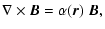
the magnetic energy density dominates over the thermal, kinetic and gravitational energy densities. This implies that, if appreciable currents are present, these must be aligned with the magnetic field, otherwise the resulting Lorentz forces could not be balanced by the non-magnetic forces. Thus, the magnetic field must be approximately force-free, characterized by the equations
| |
|
 |
(1) |
| |
|
 |
(2) |
where
 denotes a scalar function of position
  which, because of Eq. (2), is constant along the magnetic field lines. This approximation is presumably valid from the upper chromosphere
up to heights of
which, because of Eq. (2), is constant along the magnetic field lines. This approximation is presumably valid from the upper chromosphere
up to heights of 
 above the level of the photosphere in the corona
(see Gary 2001, for a careful study of the height variation of the plasma
above the level of the photosphere in the corona
(see Gary 2001, for a careful study of the height variation of the plasma  ,
i.e. the ratio between the thermal and magnetic pressures or energy densities).
,
i.e. the ratio between the thermal and magnetic pressures or energy densities).
Solutions to Eqs. (1)-(2) for the special case of a spatially constant  were given by Nakagawa & Raadu (1972), Chiu & Hilton (1977), Seehafer (1978), Alissandrakis (1981), and Semel (1988); see also reviews by Seehafer & Staude (1983), Gary (1989), and Sakurai (1989). The practical application to solar active regions
has been largely confined to these constant-
or linear force-free fields, whose determination leads to boundary value problems for a linear partial differential equation.
The extrapolations with constant-
force-free fields, as well as those with current-free fields, have provided new insights into the physics of the activity phenomena. In particular, results were obtained on magnetic topologies favourable for flares, and on magnetic and current helicities. One example is the potential role of
separatrices made up of magnetic field lines touching the photospheric boundary from above
for the formation of electric current sheets, and the fast release of stored magnetic energy by magnetic reconnection (Seehafer 1986).
These topological elements have been termed bald patches (Titov et al. 1993; Titov & Démoulin 1999; Bungey et al. 1996). Another finding is the hemispheric sign rule
for the current helicity
were given by Nakagawa & Raadu (1972), Chiu & Hilton (1977), Seehafer (1978), Alissandrakis (1981), and Semel (1988); see also reviews by Seehafer & Staude (1983), Gary (1989), and Sakurai (1989). The practical application to solar active regions
has been largely confined to these constant-
or linear force-free fields, whose determination leads to boundary value problems for a linear partial differential equation.
The extrapolations with constant-
force-free fields, as well as those with current-free fields, have provided new insights into the physics of the activity phenomena. In particular, results were obtained on magnetic topologies favourable for flares, and on magnetic and current helicities. One example is the potential role of
separatrices made up of magnetic field lines touching the photospheric boundary from above
for the formation of electric current sheets, and the fast release of stored magnetic energy by magnetic reconnection (Seehafer 1986).
These topological elements have been termed bald patches (Titov et al. 1993; Titov & Démoulin 1999; Bungey et al. 1996). Another finding is the hemispheric sign rule
for the current helicity
 ,
namely that this quantity is predominantly negative in the northern hemisphere and positive in the southern hemisphere (Seehafer 1990).
,
namely that this quantity is predominantly negative in the northern hemisphere and positive in the southern hemisphere (Seehafer 1990).
The extrapolation methods for current-free and constant-
force-free fields require only line-of-sight magnetograms (with
remaining as a free parameter in the case of the constant-
fields).
Since the early 80s, different methods for calculating non-constant-
or nonlinear force-free fields from photospheric vector magnetograms have been proposed, and presently great efforts are being made to refine them and to improve
their applicability. These
methods include:
- -
- Direct vertical integration (Wu et al. 1985; Démoulin et al. 1992; Wu et al. 1990; Cuperman et al. 1990; Song et al. 2006).
A Cauchy or initial value problem is solved with the vertical coordinate z playing the role of time, and using the photospheric boundary conditions as the initial conditions. In addition to the photospheric field components, their horizontal derivatives are also used. However, this initial value problem is mathematically
ill-posed, since the solutions do not depend continuously on the photospheric initial values.
Therefore, the methods proposed here involve regularization or smoothing schemes.
The problem of ill-posedness also occurs for constant-
and current-free fields if these
are determined, for instance, from the values of the vertical field component Bz and its vertical derivative
 (which by use of Eq. (2) can be expressed in terms of the horizontal derivatives of the horizontal components Bx and By) at the photosphere (Seehafer & Staude 1983; Amari et al. 1998).
- -
- Grad-Rubin methods (Amari et al. 2006; Wheatland 2004; Sakurai 1981; Wheatland 2006; Amari et al. 1999,1997; Grad & Rubin 1958). An electric current-magnetic field iteration is applied with field-aligned currents calculated according to
 ,
and magnetic fields calculated by using the Bio-Savart law. The normal field component Bn is prescribed on the whole boundary and
on a part of the boundary where Bn is either positive or negative. A modification of the method for global fields was proposed by Aly & Seehafer (1993),
with the additional condition that the field be radial at an exterior source surface;
this condition is usual in global potential-field extrapolations and simulates the effect of the solar wind. Convergence of the iteration and existence
of the solution can be proven for sufficiently small
,
and magnetic fields calculated by using the Bio-Savart law. The normal field component Bn is prescribed on the whole boundary and
on a part of the boundary where Bn is either positive or negative. A modification of the method for global fields was proposed by Aly & Seehafer (1993),
with the additional condition that the field be radial at an exterior source surface;
this condition is usual in global potential-field extrapolations and simulates the effect of the solar wind. Convergence of the iteration and existence
of the solution can be proven for sufficiently small  (Bineau 1972; Boulmezaoud & Amari 2000; Kaiser et al. 2000).
Such existence proofs are not available for the other methods listed here.
(Bineau 1972; Boulmezaoud & Amari 2000; Kaiser et al. 2000).
Such existence proofs are not available for the other methods listed here.
- -
- Boundary-integral methods (He & Wang 2006; Yan & Sakurai 2000; Yan & Li 2006; Yan 2003; Yan & Sakurai 1997). The magnetic field is represented by an integral over the boundary of the considered volume
involving an auxiliary function. The problem is solved iteratively whereby the auxiliary function has to be determined such that a remaining volume integral vanishes. The magnetic vector on the photospheric boundary is used as input.
- -
- Relaxation methods (Mikic & McClymont 1994; Yang et al. 1986; Roumeliotis 1996; Valori et al. 2005). The magnetohydrodynamic equations are simulated, generally in a simplified or modified form. The equation for the fluid velocity contains a viscous dissipation term but no
external forcing terms, and the pressure term is neglected. If some energy inflow through
the boundary is allowed, this must be exceeded by the dissipative losses. Asymptotically in time, a quiescent state with a force-free magnetic field is reached. Photospheric vector magnetograms are used as boundary data.
- -
- Optimization methods (Wheatland et al. 2000; Wiegelmann 2004). A positive semidefinite functional
 of the magnetic field is minimized using a prescription for evolving .
If
of the magnetic field is minimized using a prescription for evolving .
If
 is reached,
 and
and
 are satisfied throughout the volume considered. Again, photospheric vector magnetograms are used as boundary data. An adaption of the method for the calculation
of global force-free fields in spherical geometry was proposed by Wiegelmann (2007), while extensions
to non-force-free fields, with pressure gradients and gravity included, were developed by Wiegelmann & Inhester (2003) and Wiegelmann & Neukirch (2006).
are satisfied throughout the volume considered. Again, photospheric vector magnetograms are used as boundary data. An adaption of the method for the calculation
of global force-free fields in spherical geometry was proposed by Wiegelmann (2007), while extensions
to non-force-free fields, with pressure gradients and gravity included, were developed by Wiegelmann & Inhester (2003) and Wiegelmann & Neukirch (2006).
Discussions of the nonlinear extrapolation methods are found in Aly (1989), Sakurai (1989), Amari et al. (1997), McClymont et al. (1997) and Schrijver et al. (2006).
With the exception of the direct vertical integration schemes, the nonlinear extrapolation methods
impose boundary conditions on the whole boundary of the volume in which the solution is calculated,
in practice usually a rectangular box over the magnetogram area.
For the Grad-Rubin methods, the corresponding boundary value problem is well posed (at least for
sufficiently small
and perhaps up to the uniqueness of the solution). However, these methods do not exploit the full information content of vector magnetograms.
The boundary-integral, relaxation and optimization methods prescribe the magnetic vector on the boundary. Vector magnetograms provide the boundary values for the lower, photospheric part of the boundary, while some assumption is made for the remaining parts, e.g. keeping the values of an initial potential field there fixed, so that altogether the full magnetic
vector is prescribed on the whole closed boundary. This overdetermines the force-free field. Therefore, the calculations will lead to correct solutions only if the prescribed boundary values are consistent with the condition of force-freeness. This cannot be expected, however, for several reasons. First of all, the magnetic field
is not force-free in the photosphere and in the lower chromosphere (possibly with the exception of sunspot areas, where the field is strongest). Furthermore, there are measurement errors, in particular in the transverse field components (perpendicular to the line of sight of the observer), that would destroy the compatibility of a
magnetogram with the condition of force-freeness.
One way to alleviate these problems is a preprocessing of the magnetograph data as suggested
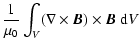
by Wiegelmann et al. (2006). The vector components of the total magnetic force and the total magnetic torque on the volume considered are given by six boundary integrals
that have to vanish if the magnetic field is force-free in the full volume (Aly 1984; Low 1985; Molodenskii 1969; Aly 1989). The preprocessing changes the boundary values
of
within the error margins of the measurement in such a way that the moduli of the six boundary integrals are minimized.
The resulting boundary values are expected to be more suitable for an extrapolation into a force-free field than the original values.
In the practical calculations, the convergence properties of the used iterations or evolutions, as well as the calculated fields themselves, are very sensitive to small-scale noise and apparent discontinuities in the photospheric magnetograph data.
This problem should, in principle, disappear if small spatial scales were sufficiently resolved. However, the numerical effort for that would be enormous.
Also, the small-scale fluctuations in the magnetograms are presumed to affect the solutions only
in a very thin boundary layer close to the photosphere.
Therefore, a smoothing of the data is included in the preprocessing.
In this paper, we follow the suggestion of Wiegelmann et al. (2006) and expand their method of preprocessing photospheric vector magnetograms.
The paper is organized as follows: in Sect. 2 we describe a new method for the preprocessing; then, in Sect. 3,
we apply it to a known nonlinear force-free test field; finally, in Sect. 4, we draw conclusions and discuss our results.
2 Procedure
The strategy of preprocessing is to define a functional L of the boundary values of ,
such that on minimizing L the total magnetic force and the total magnetic torque on the considered volume, as well as a quantity measuring the degree of small-scale noise in the boundary data,
are simultaneously made small. Each of the quantities to be made small is measured by an appropriately defined subfunctional included in L.
The different subfunctionals are weighted in order to control their relative importance.
Furthermore, domain borders are implemented so that the field is only allowed to change within these borders that are defined by the error margins of the magnetographic measurement.
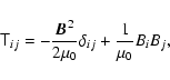
The total magnetic force on a volume V is given by
where
 is the surface of V, and in the last step Gauss' theorem was used;
 is the magnetic stress tensor,
 |
(4) |
and
 its divergence,
![\begin{displaymath}%
[{\rm div}~\tens{T}]_i=\partial_j \tens{T}_{ij}
\end{displaymath}](/articles/aa/full/2007/46/aa8454-07/img36.gif) |
(5) |
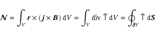
(we use the summation convention). Quite analogously,
the total magnetic torque on V can be written as
 |
(6) |
with
 |
(7) |
If, as in our case, the magnetic field is force-free in V,
the surface integrals in Eqs. (3) and (6) have to vanish.
These integrals are over the whole boundary of V, but we approximate them by integrals just over the photospheric magnetogram area. This will only be justified if the net magnetic flux through the magnetogram area vanishes (Wiegelmann et al. 2006). Actually,
 ,
,
 and
and
 are fully independent conditions, and the vanishing of the volume integrals of higher-order
moments of
are fully independent conditions, and the vanishing of the volume integrals of higher-order
moments of
 would give additional independent conditions.
Our intention is that all relevant magnetic flux is closed on the photosphere, and the field on the rest of the boundary is so weak that its contribution to the surface integrals for
would give additional independent conditions.
Our intention is that all relevant magnetic flux is closed on the photosphere, and the field on the rest of the boundary is so weak that its contribution to the surface integrals for
 and
and
 is negligible.
With S denoting the magnetogram area in the plane r3=0,
and
,
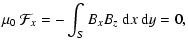
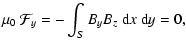
given by Eqs. (3) and (6), are then approximated by
| |
|
 |
(8) |
| |
|
 |
(9) |
where  is the unit vector in the positive r3 direction, pointing upward in the atmosphere. Writing x, y, z for the components of ,
the condition of force-freeness reads
is the unit vector in the positive r3 direction, pointing upward in the atmosphere. Writing x, y, z for the components of ,
the condition of force-freeness reads
while the condition of torque-freeness is expressed by
(see Aly 1989; Molodenskii 1969). The better these integral conditions are fulfilled, the higher is the expected compatibility of the boundary data with the requirement that the magnetic field be force-free in the volume V. However, due to their integral
character and their finite number, the conditions are only necessary, not sufficient.
Another task is to decrease the amount of small-scale irregularities in the data, which we call smoothing. One possibility here is to calculate the horizontal second-order derivatives of the photospheric field, combined in the two-dimensional Laplacian
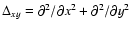 .
The square of
.
The square of
 can be used to estimate the smoothness of the photospheric boundary data because the second-order derivatives measure the curvature of the surfaces
Bx(x,y,z=0),
By(x,y,z=0) and
Bz(x,y,z=0).
Minimizing the integral of
can be used to estimate the smoothness of the photospheric boundary data because the second-order derivatives measure the curvature of the surfaces
Bx(x,y,z=0),
By(x,y,z=0) and
Bz(x,y,z=0).
Minimizing the integral of
![$\left[\Delta_{xy} \vec B(x,y,z=0)\right]^2$](/articles/aa/full/2007/46/aa8454-07/img56.gif) over the magnetogram area S is one method of averaging the field. The disadvantage here is that, if the modulus of
is decreased to zero on S, all global or local maxima or minima of the three field components
on S are removed, including the physically significant ones, and the total energy content of the field may be strongly reduced. Therefore, this method of smoothing can only be applied with great care.
over the magnetogram area S is one method of averaging the field. The disadvantage here is that, if the modulus of
is decreased to zero on S, all global or local maxima or minima of the three field components
on S are removed, including the physically significant ones, and the total energy content of the field may be strongly reduced. Therefore, this method of smoothing can only be applied with great care.
A different method of smoothing a vector magnetogram, which we prefer here, is the windowed median
(see, e.g., Press et al. 1989). In this method one chooses a small window around
a given point, calculates the median of the field values in the window, and then minimizes the difference between the field value
at the point and the median of the window. Calculating the median is a more stable way of averaging than the normal mean,
which corresponds to minimizing the Laplacian,
because it is much less influenced by strong disturbances in a small number of points. After several iterations the method will
stabilize the changes; this way, the structures of the measurement are conserved even if
the quantity minimized here is decreased to zero.
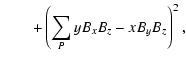
In discretized form, the squares of the total magnetic force and the total magnetic torque are given by
where the summation is over the points P of a photospheric grid.
Since there is no obvious reason to weight L1 and L2 differently,
they are combined to
This can only be done if the two quantities have been made dimensionless beforehand.
We normalize L1 to
![\begin{displaymath}%
N_{L_1} = \left[ \sum_P \left(\vec{B}^{(0)}\right)^2 \right]^2
=B_{{\rm mean}}^4 N^2,
\end{displaymath}](/articles/aa/full/2007/46/aa8454-07/img60.gif) |
(19) |
where
 is the original, magnetographically measured photospheric field,
 the mean value of
 over the magnetogram, and N the number of photospheric
grid points, and we normalize L2 to
over the magnetogram, and N the number of photospheric
grid points, and we normalize L2 to
![\begin{displaymath}%
N_{L_2} \!=\! \left[\sum_P \sqrt{x^2\!+\!y^2} \left(\vec{B}...
...t{k^2\!+\!l^2}
\left(\vec{B}^{(0)}_{kl}\right)^2 \right]^2\!,
\end{displaymath}](/articles/aa/full/2007/46/aa8454-07/img64.gif) |
(20) |
with Nx and Ny denoting the numbers of grid points in the x and y directions (
 ), h the grid spacing (assumed to be equal in the x and y directions) and
 the elements of the magnetogram
matrix. With these normalizations, L1 and L2 are independent of the units of length and magnetic field and both are 1 for a field that is neither force-free nor torque-free.
the elements of the magnetogram
matrix. With these normalizations, L1 and L2 are independent of the units of length and magnetic field and both are 1 for a field that is neither force-free nor torque-free.
The smoothing functional is defined as![[*]](/icons/foot_motif.gif)
 |
|
|
|
![$\displaystyle \left.\left.\dots,B_i(x+n\cdot h,y+n\cdot h)\right] - B_i(x,y) \right\}^2,$](/articles/aa/full/2007/46/aa8454-07/img68.gif) |
|
|
(21) |
where n is a positive integer number and Mn the median of a rectangular window with
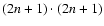 grid points centered about the point (x,y). The values at the boundary of the magnetogram, where the method does not work, are left
unchanged; these values are expected to be small in general. Also, in the practical extrapolations an artificial margin where the field vanishes is very often added to the magnetogram.
L4 is normalized to
grid points centered about the point (x,y). The values at the boundary of the magnetogram, where the method does not work, are left
unchanged; these values are expected to be small in general. Also, in the practical extrapolations an artificial margin where the field vanishes is very often added to the magnetogram.
L4 is normalized to
 |
|
|
|
![$\displaystyle \left.\left.\dots, B_i^{(0)}(x+n\cdot h,y+n\cdot h)\right] + B_i^{(0)}(x,y) \right\}^2,$](/articles/aa/full/2007/46/aa8454-07/img71.gif) |
|
|
(22) |
so that  for a field of maximum roughness.
Since just the relative weighting of the different subfunctionals is important for the minimization, the weighting of one of them can be set as equal to unity. We choose the form
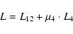 |
(23) |
for the total functional to minimize. Like the number n determining the window size for the smoothing, the weighting factor  is yet undetermined.
Minimizing a simple functional with just one minimum can be easily done
by fast methods like Newton-Raphson iteration, but here we have a more
complex functional and, to our knowledge, there is no way of knowing how
many local minima exist or if there actually exists a global minimum. The
success of the Newton-Raphson method strongly depends on the initial
field for the iteration, since it just finds the nearest local minimum.
We use here the method of simulated annealing (see,
e.g., Corana et al. 1987; Press et al. 1989; Siarry et al. 1997; Rutenbar 1989), which also finds the
nearest local minimum, but opens a chance to leave it and to find
a deeper one, within given domain borders.
Simulated annealing works as follows: start with a given field and
change the values of the vector components at one grid point randomly
within a small interval (for example 0.5% around the initial values).
Then calculate the functional that has to be minimized both for the
initial and the changed field. If the new value of the functional,
 ,
is smaller than the old one,
,
is smaller than the old one,
 ,
then take the new field. If the new value is larger than the old one, then
take the new field with a probability
,
then take the new field. If the new value is larger than the old one, then
take the new field with a probability 
 ,
where the "temperature'' T is used to control the behaviour of the algorithm. A sweep through the whole magnetogram is one iteration. Use the chosen field as the initial field for the next iteration.
Start the algorithm with small values of T; this way, only smaller
values of L will be accepted. After some iterations a
first minimum is reached. Increase the value of T; this way one
opens a chance of leaving the first minimum.
If the minimum has been left, decrease T again and the
algorithm will again find the nearest local minimum. In this way, the
whole domain, as defined by the domain borders, will be scanned (changes
to field values outside the domain borders defined before are not allowed).
,
where the "temperature'' T is used to control the behaviour of the algorithm. A sweep through the whole magnetogram is one iteration. Use the chosen field as the initial field for the next iteration.
Start the algorithm with small values of T; this way, only smaller
values of L will be accepted. After some iterations a
first minimum is reached. Increase the value of T; this way one
opens a chance of leaving the first minimum.
If the minimum has been left, decrease T again and the
algorithm will again find the nearest local minimum. In this way, the
whole domain, as defined by the domain borders, will be scanned (changes
to field values outside the domain borders defined before are not allowed).
![\begin{figure}
\includegraphics[width=6cm,height=6cm]{8454fg1a.eps}\includegrap...
...454fg1h.eps}\includegraphics[width=6cm,height=6cm]{8454fg1i.eps}\\
\end{figure}](/articles/aa/full/2007/46/aa8454-07/Timg78.gif) |
Figure 1:
Top row: magnetogram derived from the Low & Lou test field. From left to right the three components Bx, By, Bz are shown.
Middle row: the same magnetogram as in the first row, but with noise added (for details see the main text). Bottom row: magnetogram resulting from preprocessing of the disturbed magnetogram shown in the second row. |
| Open with DEXTER |
3 Application to the Low and Lou test field
In order to test our preprocessing technique, we used one of the semi-analytical solutions found by
Low & Lou (1990). These have become standard test cases for extrapolations of nonlinear force-free
magnetic fields (cf. Amari et al. 2006; Wheatland et al. 2000; Wiegelmann 2004; Wiegelmann et al. 2006; Schrijver et al. 2006; Valori et al. 2007). We chose a frequently used special solution,
characterized by the parameters n=1, m=1, l = 0.3 and
 ;
for details see Low & Lou (1990). The field was given
in the cubic volume
;
for details see Low & Lou (1990). The field was given
in the cubic volume
 ,
,
 ,
,
 ,
so the test field is
identical to FF1 in Amari et al. (2006) and Case I in Schrijver et al. (2006) and Valori et al. (2007).
We used a numerical resolution of 643 grid points, and the unit for the magnetic field was chosen such that the maximum strength of the photospheric normal component is 1000 G.
,
so the test field is
identical to FF1 in Amari et al. (2006) and Case I in Schrijver et al. (2006) and Valori et al. (2007).
We used a numerical resolution of 643 grid points, and the unit for the magnetic field was chosen such that the maximum strength of the photospheric normal component is 1000 G.
![\begin{figure}
\par\includegraphics[width=6cm,height=6cm]{8454fg2a.eps}\includeg...
...m]{8454fg2b.eps}\includegraphics[width=6cm,height=6cm]{8454fg2c.eps}\end{figure}](/articles/aa/full/2007/46/aa8454-07/Timg83.gif) |
Figure 2:
Evolution of the total functional L ( left) and of the subfunctionals L12 ( center) and L4 ( right) in the course of the minimization on a logarithmic scale. All three quantities are normalized to their initial values. |
| Open with DEXTER |
![\begin{figure}
\par\includegraphics[width=6cm,height=6cm]{8454fg3a.eps}\includeg...
...m]{8454fg3b.eps}\includegraphics[width=6cm,height=6cm]{8454fg3c.eps}\end{figure}](/articles/aa/full/2007/46/aa8454-07/Timg84.gif) |
Figure 3:
Contours of the function
 for the undisturbed magnetogram ( left; magnetogram shown in top row of Fig. 1), the disturbed magnetogram ( center; magnetogram shown in middle row of Fig. 1) and the preprocessed magnetogram ( right; magnetogram shown in bottom row of Fig. 1).
 |
| Open with DEXTER |
3.1 Contours of the magnetogram
In the top row of Fig. 1, from left to right the three components Bx, By, Bz of a vector magnetogram derived from the Low & Lou test field are shown.
The middle row shows the same magnetogram, but now with artificial noise. At every grid point of the magnetogram white noise was added, based on a relative error of 30% in
the horizontal field components and 5% in the normal component,
corresponding to the fact that the measurement of the transverse field components is much less accurate than that of the line-of-sight component (we consider a case where the z direction coincides with the line of sight). Additionally, we assumed a field-independent error component (also white noise) with an absolute (maximum) amplitude of 35 G in all three field components.
Starting from the disturbed magnetogram we applied our preprocessing as described in Sect. 2. The smoothing was weighted with a factor of
 in the functional L (see Sect. 3.4 for a discussion of how to find an optimal value for )
and carried out using the windowed median method with n=1.
The domain borders for the minimization by the method of simulated annealing were chosen to be 85 G for the transverse components and 35 G for the normal component.
in the functional L (see Sect. 3.4 for a discussion of how to find an optimal value for )
and carried out using the windowed median method with n=1.
The domain borders for the minimization by the method of simulated annealing were chosen to be 85 G for the transverse components and 35 G for the normal component.
In the bottom row of Fig. 1 the preprocessed magnetogram is shown.
Comparison with the original undisturbed magnetogram (top row of the figure) shows that the method works remarkably well. The neutral lines where the respective field components change sign, as well as the poles (minima and maxima), are mainly recovered.
Also, the small-scale noise in the disturbed magnetogram (middle row
of the figure) has been removed.
In Fig. 2 the evolutions of L and of the two subfunctionals L12 and L4 (cf. Sect. 2) in the course of the minimization are shown.
All three quantities are normalized to their initial values in order to show, in particular, the decrease related to the initial values. As one can see, after 100 iterations the algorithm first found a local minimum of L, but then it drove the system out of this
minimum to find one where, in particular, L12 is smaller by an order of magnitude.
The function
defined by Eq. (1) contains much information on the
topology of the magnetic field lines since these lie in the surfaces
 .
In particular, the values of
at any two points in the photosphere that are connected by a field line above the photosphere must be identical.
For the level of the photosphere,
can be calculated from the magnetogram according to
.
In particular, the values of
at any two points in the photosphere that are connected by a field line above the photosphere must be identical.
For the level of the photosphere,
can be calculated from the magnetogram according to
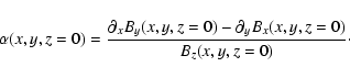 |
(24) |
Obviously, since one has to combine three noisy quantities and, moreover, to differentiate two of them,
is more sensitive to noise in the magnetographic measurement than the field components themselves. In Fig. 3, from left to right the function
is shown as calculated from the undisturbed magnetogram derived from the Low & Lou field, the disturbed magnetogram and the preprocessed magnetogram (cf. Sect. 3.1).
The noise overshadows the signal of
strongly. However, the preprocessing is even able to recover the main structures of this heavily disturbed function.
A critical test of the effect of the preprocessing is to extrapolate from disturbed photospheric vector magnetograms before and after the preprocessing, and compare the
results with those of extrapolations starting from the exact photospheric values of the Low & Lou test solution, as well as with the exact field values of this solution in the volume above the photosphere. We used the magneto-frictional relaxation method of Valori et al. (2005) (see also Valori et al. 2007) for corresponding extrapolations.
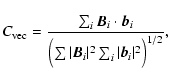
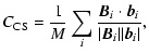
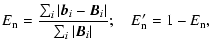
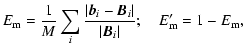
To assess the quality of extrapolations, Schrijver et al. (2006) developed a number of figures of merit (hereafter FoM). The FoM are measures of the discrepancy between an exactly known test field, ,
and the extrapolated field,  ,
namely
,
namely
where M is the number of grid points in the considered three-dimensional domain and the summation is over these grid points.
 is the scalar product between the unit vectors corresponding to
and ,
respectively, in the
3M-dimensional space spanned by the field values of the whole grid, and
is the scalar product between the unit vectors corresponding to
and ,
respectively, in the
3M-dimensional space spanned by the field values of the whole grid, and
 is the mean value over the grid of the scalar products between the unit vectors of the two fields in three-dimensional space.
 and
and
 measure the vector error
 with a global and a local normalization,
respectively, and
with a global and a local normalization,
respectively, and
 is the ratio between the magnetic energies of the extrapolated and exact fields.
![\begin{figure}
\par\includegraphics[width=7.1cm,clip]{8454fig4.eps}\end{figure}](/articles/aa/full/2007/46/aa8454-07/Timg97.gif) |
Figure 4:
Figures of merit
,
,
 , ,
 and
(from left to right) for three-dimensional fields
extrapolated from the original magnetogram with the exact field values of the Low & Lou solution (blue; magnetogram shown in top row of Fig. 1), the disturbed magnetogram (green; magnetogram shown in middle row of Fig. 1) and the preprocessed magnetogram
(red; magnetogram shown in bottom row of Fig. 1).
and
(from left to right) for three-dimensional fields
extrapolated from the original magnetogram with the exact field values of the Low & Lou solution (blue; magnetogram shown in top row of Fig. 1), the disturbed magnetogram (green; magnetogram shown in middle row of Fig. 1) and the preprocessed magnetogram
(red; magnetogram shown in bottom row of Fig. 1). |
| Open with DEXTER |
In Fig. 4, the FoM are shown for three-dimensional fields extrapolated from a magnetogram containing the exact field values of the Low & Lou solution,
a noisy magnetogram obtained from this as described in Sect. 3.1, and a magnetogram obtained by applying our preprocessing procedure to the noisy magnetogram. Instead of
and
,
(see Eq. (27)) and
(see Eq. (28)) are shown, so that all displayed measures are equal to unity in the case of a full match. Naturally, the extrapolation of the original magnetogram reproduces the exact field best. The agreement is markedly worse for the extrapolation of the noisy magnetogram, but is again significantly improved for the extrapolation using the preprocessed magnetogram. Only the energy ratio
shows a deviating behaviour. The reduced energy content of the
field extrapolated from the preprocessed magetogram compared to that extrapolated from the noisy magnetogram can be explained by the smoothing procedure, which removes a part of the energy in the small spatial scales. That the noisy magnetogram gives a higher energy content of the field than the undisturbed one seems to be mainly a result of our addition of a noise component with field-independent amplitude (cf. Sect. 3.1),
which increases, in particular, the energy in the weak-field regions.
3.4 Searching for an optimal
The expression for the minimization functional L, given by
Eq. (23), contains the free parameter .
If  ,
the subfunctional L12, measuring the deviation from force-freeness and torque-freeness, is minimized very effectively. For our noisy test magnetogram generated from the Low & Lou solution and with the chosen domain borders for the minimization, the value of the subfunctional L12 is decreased to zero
(within machine accuracy) relatively quickly.
For
,
the subfunctional L12, measuring the deviation from force-freeness and torque-freeness, is minimized very effectively. For our noisy test magnetogram generated from the Low & Lou solution and with the chosen domain borders for the minimization, the value of the subfunctional L12 is decreased to zero
(within machine accuracy) relatively quickly.
For
 ,
L12=0 is no longer reached. This results from a competition between two different minimization objectives. Increasing
gives L4 a higher weight and, thus, enforces the smoothing and inhibits the decrease of L12. On
the other hand, decreasing
gives L12 the possibility to
reach values close to zero, but inhibits the smoothing. So L12 and L4 are competitive functionals, and finding the right
is an optimization problem on its own.
,
L12=0 is no longer reached. This results from a competition between two different minimization objectives. Increasing
gives L4 a higher weight and, thus, enforces the smoothing and inhibits the decrease of L12. On
the other hand, decreasing
gives L12 the possibility to
reach values close to zero, but inhibits the smoothing. So L12 and L4 are competitive functionals, and finding the right
is an optimization problem on its own.
Unfortunately, there is no simple way to determine an optimum .
One could extrapolate from magnetograms derived from a test field and compare the extrapolated fields with the exact solution. However, the numerical effort for this would be very high and the result would only be valid for the test field.
Since L (see Eq. (23)) depends on ,
it seems better to look at a different functional that is independent of
to investigate the influence of different weightings on the minimization process. The simplest choice for such a functional is the sum
L12+L4.
It is then, in principle, possible to find an optimal
by the method
of simulated annealing. Thus, one can minimize L for different values of and then compare the values of
L12+L4 for the associated photospheric magnetic fields
that minimize L, i.e., one compares the sums
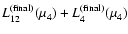 of the final values of L12 and L4 reached by the minimization of L for different values of .
At the same time, in view of the arbitrariness of the choice
L12+L4, the dependence of the final
values of the two individual subfunctionals L12 and L4 should be considered.
of the final values of L12 and L4 reached by the minimization of L for different values of .
At the same time, in view of the arbitrariness of the choice
L12+L4, the dependence of the final
values of the two individual subfunctionals L12 and L4 should be considered.
![\begin{figure}
\par\includegraphics[width=7.4cm,clip]{8454fig5.eps}\end{figure}](/articles/aa/full/2007/46/aa8454-07/Timg101.gif) |
Figure 5:
Dependence of the final values of L12, L4 and
L12+L4 on the parameter
on a doubly logarithmic scale. The values were calculated by applying the minimization procedure for L to the noisy magnetogram
(shown in middle row of Fig. 1) generated from the Lou & Lou test solution. |
| Open with DEXTER |
In Fig. 5, the dependence of the final values of L12, L4 and
L12+L4 on
is shown. The calculations were done using the
noisy magnetogram generated from the Low & Lou test solution (cf. Sect. 3.1).
One can see that
reaches a broad
minimum in the interval
 .
We have chosen ,
a value at the left border of this interval, for our
calculations (cf. Sect. 3.1), in doing this a low final value of L12 is found
and the final value of L4 has reached a saturation, decreasing only slightly for further increased values of .
.
We have chosen ,
a value at the left border of this interval, for our
calculations (cf. Sect. 3.1), in doing this a low final value of L12 is found
and the final value of L4 has reached a saturation, decreasing only slightly for further increased values of .
4 Conclusions
We have developed a new method for the preprocessing of solar photospheric vector magnetograms that
makes them more suitable for extrapolations into three-dimensional nonlinear force-free magnetic fields in the chromosphere and corona. The principle of the method is the one suggested by
Wiegelmann et al. (2006), namely, to minimize a functional, L, of the photospheric field values
whereby the total magnetic force and the total magnetic torque on the considered volume
above the photosphere, as well as a quantity measuring the degree of small-scale noise in the photospheric boundary data, are simultaneously made small.
For the minimization we use the method of simulated annealing. Compared to methods like Newton-Raphson iteration, this method has the advantage of finding not only the local minimum closest to the chosen initial field, but also of absolutely minimizing the functional L.
The smoothing of noisy magnetograph data is performed by windowed median averaging. Compared to other methods in use, this method of averaging better conserves the real structures in the measurements.
We have applied our method of preprocessing to a magnetogram derived from one of the semi-analytical
nonlinear force-free magnetic fields devised by Low & Lou (1990). The magnetogram was exposed to an artificial noise. The algorithm recovered all main structures of the magnetogram and removed small-scale noise. Even quantities that are very sensitive to noise, like the function
in the plane of the magnetogram,
could be reproduced very well. The main test of the effect of the preprocessing was to extrapolate from the noisy photospheric vector magnetogram before and after the preprocessing, and compare the
results with those of extrapolations starting from the exact photospheric values of the Low & Lou test solution, as well as with the exact field values of this solution itself. To assess
the quality of the extrapolations, the figures of merit developed by Schrijver et al. (2006) were used.
The preprocessing was found to significantly improve the agreement of the extrapolated field with the exact field.
The method of minimization by simulated annealing is easy to adjust to special requirements,
such as changed or new minimization objectives, since the functional L is treated directly, i.e., only the values of the functional itself have to be calculated. In contrast with, e.g., Newton-Raphson iteration, derivatives of L are not needed.
Our minimization functional contains a free weighting parameter, ,
that controls the relative influence of the requirements of force-freeness and torque-freeness on the one hand, and smoothness of the photospheric field on the other hand. We have outlined a way to find an optimal value of .
The original motivation for the preprocessing was to make vector magnetograph data more suitable for extrapolation methods that prescribe the full magnetic vector on the whole closed boundary of the considered volume, such as the relaxation and optimization methods, since prescribing the full vector overdetermines the force-free field. Making the the magnetograms more compatible with the condition of force-freeness can also be useful for extrapolations with Grad-Rubin methods since, e.g., the values of the function
,
which are determined from the magnetogram on a part of the photospheric boundary,
must be identical at the photospheric end points of a field line. Moreover, the determination
of
is very sensitive to noise, so that a smoothing of the data, as done by our
method, also appears advisable. Finally, smoothing of the magnetograms is an indispensable part of extrapolations by direct
vertical integration, since small-scale errors can grow exponentially with height. Thus, our method
of smoothing could also be useful for this kind of extrapolation.
Acknowledgements
This work was supported by the Deutsche Forschungsgemeinschaft (DFG)
through grants HO 1424/9-1 and SE 662/11-1.
- Alissandrakis, C. E.
1981, A&A, 100, 197 [NASA ADS]
(In the text)
- Altschuler,
M. D., & Newkirk, Jr., G. 1969, Sol. Phys., 9,
131 [NASA ADS] [CrossRef]
- Aly, J. J. 1984,
ApJ, 238, 349 [NASA ADS] [CrossRef]
- Aly, J. J. 1989,
Sol. Phys., 120, 19 [NASA ADS] [CrossRef]
(In the text)
- Aly, J. J.,
& Seehafer, N. 1993, Sol. Phys., 144, 243 [NASA ADS] [CrossRef]
(In the text)
- Amari, T., Aly,
J. J., Luciani, J. F., Boulmezaoud, T. Z., &
Mikic, Z. 1997, Sol. Phys., 174, 129 [NASA ADS] [CrossRef]
- Amari, T.,
Boulmezaoud, T. Z., & Maday, Y. 1998, A&A, 339,
252 [NASA ADS]
- Amari, T.,
Boulmezaoud, T. Z., & Mikic, Z. 1999, A&A, 350,
1051 [NASA ADS]
- Amari, T.,
Boulmezaoud, T. Z., & Aly, J. J. 2006, A&A, 446,
691 [NASA ADS] [CrossRef] [EDP Sciences]
- Bineau, M. 1972, Comm.
Pure Appl. Math., 25, 77
- Boulmezaoud,
T. Z., & Amari, T. 2000, Z. angew. Math. Phys., 51,
942 [CrossRef]
- Bungey,
T. N., Titov, V. S., & Priest, E. R. 1996,
A&A, 308, 233 [NASA ADS]
- Chiu, Y. T.,
& Hilton, H. H. 1977, ApJ, 212, 873 [NASA ADS] [CrossRef]
(In the text)
- Corana, A.,
Marchesi, M., Martini, C., & Ridella, S. 1987, ACM Transactions
on Mathematical Software (TOMS), 13, 262
- Cuperman, S.,
Ofman, L., & Semel, M. 1990, A&A, 230, 193 [NASA ADS]
-
Démoulin, P., Cuperman, S., & Semel, M. 1992, A&A,
263, 351 [NASA ADS]
- Gary, G. A. 1989,
ApJS, 69, 323 [NASA ADS] [CrossRef]
(In the text)
- Gary, G. A. 2001,
Sol. Phys., 203, 71 [NASA ADS] [CrossRef]
(In the text)
- Grad, H., &
Rubin, H. 1958, in Proc. 2nd Int. Conf. Peaceful Uses of Atomic
Energy (Geneva: United Nations), 31, 190
- He, H., & Wang,
H. 2006, MNRAS, 369, 207 [NASA ADS]
- Kaiser, R.,
Neudert, M., & von Wahl, W. 2000, Commun. Math. Phys., 211,
111 [NASA ADS] [CrossRef]
- Low, B. C. 1985, in
Measurements of Solar Vector Magnetic Fields, ed. M. J.
Hagyard, NASA Conf. Publ., 2374, 49
- Low, B. C.,
& Lou, Y. Q. 1990, ApJ, 352, 343 [NASA ADS] [CrossRef]
(In the text)
- McClymont,
A. N., Jiao, L., & Mikic, Z. 1997, Sol. Phys., 174,
191 [NASA ADS] [CrossRef]
(In the text)
- Mikic, Z., &
McClymont, A. N. 1994, in Solar Active Region Evolution:
Comparing Models with Observations, ed. K. S.
Balasubramaniam, & G. W. Simon (San Francisco: ASP),
ASP Conf. Ser., 68, 225
- Molodenskii, M. M.
1969, Soviet Ast., 12, 585 [NASA ADS]
- Nakagawa, Y., &
Raadu, M. A. 1972, Sol. Phys., 25, 127 [NASA ADS] [CrossRef]
(In the text)
- Press, W. H.,
Flannery, B. P., Teukolsky, S. A., & Vetterling,
W. T. 1989, Numerical Recipes, The Art of Scientific
Computing, FORTRAN Version (Cambridge, England: Cambridge
University Press)
(In the text)
- Roumeliotis, G. 1996,
ApJ, 473, 1095 [NASA ADS] [CrossRef]
- Rutenbar, R. A.
1989, Circuits and Devices Magazine, IEEE, 5, 19
- Sakurai, T. 1981,
Sol. Phys., 69, 343 [NASA ADS] [CrossRef]
- Sakurai, T. 1989, Space
Sci. Rev., 51, 11 [NASA ADS]
(In the text)
- Schatten,
K. H., Wilcox, J. M., & Ness, N. F. 1969,
Sol. Phys., 6, 442 [NASA ADS] [CrossRef]
- Schmidt, H. U. 1964,
in AAS/NASA Symposium on the Physics of Solar Flares,
ed. W. N. Hess, NASA SP-50 (Washington, D.C.: NASA),
107
- Schrijver,
C. J., DeRosa, M. L., Metcalf, T. R., et al.
2006, Sol. Phys., 235, 161 [NASA ADS] [CrossRef]
(In the text)
- Seehafer, N. 1978,
Sol. Phys., 58, 215 [NASA ADS] [CrossRef]
(In the text)
- Seehafer, N. 1986,
Sol. Phys., 105, 223 [NASA ADS] [CrossRef]
(In the text)
- Seehafer, N. 1990,
Sol. Phys., 125, 219 [NASA ADS] [CrossRef]
(In the text)
- Seehafer, N., &
Staude, J. 1983, Phys. Solariterr., 22, 5
(In the text)
- Semel, M. 1988, A&A,
198, 293 [NASA ADS]
(In the text)
- Siarry, P.,
Berthiau, G., Durdin, F., & Haussy, J. 1997, ACM Transactions
on Mathematical Software (TOMS), 23, 209
- Song, M. T.,
Fang, C., Tang, Y. H., Wu, S. T., & Zhang, Y. A.
2006, ApJ, 649, 1084 [NASA ADS] [CrossRef]
- Teuber, D.,
Tandberg-Hanssen, E., & Hagyard, M. J. 1977,
Sol. Phys., 53, 97 [NASA ADS] [CrossRef]
- Titov, V. S.,
& Démoulin, P. 1999, A&A, 351, 707 [NASA ADS]
- Titov,
V. S., Priest, E. R., & Démoulin, P. 1993,
A&A, 276, 564 [NASA ADS]
- Valori, G.,
Kliem, B., & Fuhrmann, M. 2007, Sol. Phys.,
in press
- Valori, G.,
Kliem, B., & Keppens, R. 2005, A&A, 433, 335 [NASA ADS] [CrossRef] [EDP Sciences]
- Wheatland, M. S.
2004, Sol. Phys., 222, 247 [NASA ADS] [CrossRef]
- Wheatland, M. S.
2006, Sol. Phys., 238, 29 [NASA ADS] [CrossRef]
- Wheatland,
M. S., Sturrock, P. A., & Roumeliotis, G. 2000, ApJ,
540, 1150 [NASA ADS] [CrossRef]
- Wiegelmann, T. 2004,
Sol. Phys., 219, 87 [NASA ADS] [CrossRef]
- Wiegelmann, T. 2007,
Sol. Phys., 240, 227 [NASA ADS] [CrossRef]
(In the text)
- Wiegelmann, T.,
& Inhester, B. 2003, Sol. Phys., 214, 287 [NASA ADS] [CrossRef]
(In the text)
- Wiegelmann, T.,
& Neukirch, T. 2006, A&A, 457, 1053 [NASA ADS] [CrossRef] [EDP Sciences]
(In the text)
- Wiegelmann,
T., Inhester, B., & Sakurai, T. 2006, Sol. Phys., 233,
215 [NASA ADS] [CrossRef]
(In the text)
- Wu, S. T.,
Chang, H. M., & Hagyard, M. J. 1985, in Measurements
of Solar Vector Magnetic Fields, ed. M. J. Hagyard, NASA
Conf. Publ., 2374, 17
- Wu, S. T.,
Sun, M. T., Chang, H. M., Hagyard, M. J., &
Gary, G. A. 1990, ApJ, 362, 698 [NASA ADS] [CrossRef]
- Yan, Y. 2003, Space Sci.
Rev., 107, 119 [NASA ADS] [CrossRef]
- Yan, Y., & Li, Z.
2006, ApJ, 638, 1162 [NASA ADS] [CrossRef]
- Yan, Y., &
Sakurai, T. 1997, Sol. Phys., 174, 65 [NASA ADS] [CrossRef]
- Yan, Y., &
Sakurai, T. 2000, Sol. Phys., 195, 89 [NASA ADS] [CrossRef]
- Yang,
W. H., Sturrock, P. A., & Antiochos, S. K. 1986,
ApJ, 309, 383 [NASA ADS] [CrossRef]
Copyright ESO 2007










![\begin{figure}
\includegraphics[width=6cm,height=6cm]{8454fg1a.eps}\includegrap...
...454fg1h.eps}\includegraphics[width=6cm,height=6cm]{8454fg1i.eps}\\
\end{figure}](/articles/aa/full/2007/46/aa8454-07/img78.gif)
![\begin{figure}
\par\includegraphics[width=6cm,height=6cm]{8454fg2a.eps}\includeg...
...m]{8454fg2b.eps}\includegraphics[width=6cm,height=6cm]{8454fg2c.eps}\end{figure}](/articles/aa/full/2007/46/aa8454-07/img83.gif)
![\begin{figure}
\par\includegraphics[width=6cm,height=6cm]{8454fg3a.eps}\includeg...
...m]{8454fg3b.eps}\includegraphics[width=6cm,height=6cm]{8454fg3c.eps}\end{figure}](/articles/aa/full/2007/46/aa8454-07/img84.gif)

![\begin{figure}
\par\includegraphics[width=7.1cm,clip]{8454fig4.eps}\end{figure}](/articles/aa/full/2007/46/aa8454-07/img97.gif)
![\begin{figure}
\par\includegraphics[width=7.4cm,clip]{8454fig5.eps}\end{figure}](/articles/aa/full/2007/46/aa8454-07/img101.gif)