 ,
where a is the isothermal speed of sound. Left in abeyance,
therefore,
was the question of matching to solutions
describing the highly supersonic, spherically-symmetric winds where P Cygni
lines are formed.
,
where a is the isothermal speed of sound. Left in abeyance,
therefore,
was the question of matching to solutions
describing the highly supersonic, spherically-symmetric winds where P Cygni
lines are formed.
A&A 474, 701-706 (2007)
DOI: 10.1051/0004-6361:20078236
L. B. Lucy
Astrophysics Group, Blackett Laboratory, Imperial College London, Prince Consort Road, London SW7 2AZ, UK
Received 6 July 2007 / Accepted 11 September 2007
Abstract
Following procedures pioneered by Castor et al.
(1975, ApJ, 195, 157, [CAK]), spherically-symmetric supersonic winds for O stars are computed
for matching to plane-parallel moving reversing layers (RL's) from
Paper I (Lucy 2007, A&A, 468, 649).
In contrast to a CAK wind, each of these solutions is singularity-free, thus
allowing its mass-loss rate to be fixed by the regularity condition at
the sonic point within the RL. Moreover,
information propagation in these winds by radiative-acoustic waves is
everywhere outwardly-directed, justifying the implicit assumption in Paper I that
transonic flows are unaffected by inwardly-directed wave motions.
Key words: stars: early-type - stars: mass-loss - stars: winds, outflows
In a recent paper (Lucy 2007, [Paper I]), models of moving reversing layers (RL's) for O stars were used to investigate the role of photospheric turbulence in regulating the mass flux J that can be accelerated to supersonic velocities. According to the underlying theory, the integro- differental equations describing stationary plane-parallel outflow have J as an eigenvalue, and this is determined by demanding regularity at the sonic point (Lucy & Solomon 1970).
The solutions in Paper I were followed to velocities
,
where a is the isothermal speed of sound. Left in abeyance,
therefore,
was the question of matching to solutions
describing the highly supersonic, spherically-symmetric winds where P Cygni
lines are formed.
Many investigators of line-driven winds follow Castor et al.
(1975, [CAK]) in using the Sobolev approximation to compute  ,
the radiation force per gm due to lines. Since this approximation is valid
at the highest velocites reached by the solutions in Paper I,
continuation to
,
the radiation force per gm due to lines. Since this approximation is valid
at the highest velocites reached by the solutions in Paper I,
continuation to
 with a CAK solution would seem to be
appropriate. But matching a CAK wind to a moving-RL is in general impossible.
Given a star's basic parameters,
namely composition, mass
with a CAK solution would seem to be
appropriate. But matching a CAK wind to a moving-RL is in general impossible.
Given a star's basic parameters,
namely composition, mass  ,
radius R and luminosity L, the
regularity condition at the CAK critical point
admits only one solution, with mass-loss rate
,
radius R and luminosity L, the
regularity condition at the CAK critical point
admits only one solution, with mass-loss rate
 as its
eigenvalue. Since the moving-RL already specifies that
as its
eigenvalue. Since the moving-RL already specifies that
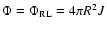 ,
we will in general find that
,
we will in general find that
 .
.
This matching problem is the topic of this paper. At first sight, there are
two approaches. If the moving-RL is the accepted starting point,
then continuation to higher
velocities requires solution of the basic integro-differential system
since a CAK singularity then no longer exists (Lucy 1975) and so
 is not constrained by a regularity condition at supersonic velocity.
On the other hand, if the unique CAK solution is the accepted
starting point, then some mechanism must be identified that can force a
structural adjustment of the RL so that
is not constrained by a regularity condition at supersonic velocity.
On the other hand, if the unique CAK solution is the accepted
starting point, then some mechanism must be identified that can force a
structural adjustment of the RL so that
 .
.
This paper's basic premise is that the critical point that determines the
eigenvalue
of a stationary line-driven wind is the sonic point and not
the CAK critical point. In this section, therefore, a model of the
spherically-symmetric supersonic zone is developed for matching to the
plane-parallel sub- and transonic models of Paper I.
Given that the aim is to resolve the paradox of two distict procedures for
predicting ,
a fairly simple model is adopted: numerical
precision is surely not needed to settle a question of principle. Accordingly,
the supersonic wind is assumed to be isothermal with
 and H and
  are assumed to be full ionized.
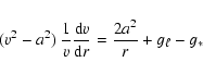
With sphericity now included, the equation of continuity has the integral
 |
(1) |
 |
(2) |
 .
.
In Sect. 1, a plausible argument was given that the calculation of
must be based
on non-Sobolev transfer since otherwise a CAK singularity will be
encountered in the supersonic flow.
Notwithstanding this argument,
is now derived using the Sobolev
approximation. The assumptions are as follows:
by means of an analytic force multiplier function M(t) is
not followed. This approximation has the merit of computational
economy and, more importantly, allows a fairly straightforward analysis of
solution
domains and singular points. But this analysis becomes significantly
more complicated when CF is included, and yet further complicated when the
M(t) parameters vary with radius as in WM-basic models
(Pauldrach et al. 2001). Accordingly, the force multiplier approach
is dropped and replaced by direct summation.
 |
(3) |
 |
(4) |
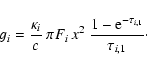
 is the flux emitted at the line's
rest frequency
is the flux emitted at the line's
rest frequency  by the photosphere located at
x = R/r = 1.
Line formation
is accounted for through the factor containing the Sobolev optical depth
given by
by the photosphere located at
x = R/r = 1.
Line formation
is accounted for through the factor containing the Sobolev optical depth
given by
![\begin{displaymath}\tau_{i,1} = \frac{\kappa_{i} \rho c}{\nu_{i}} \:/
\left[\mu...
...frac{{\rm d}v}{{\rm d}r} + (1-\mu_{1}^{2}) \frac{v}{r} \right]
\end{displaymath}](/articles/aa/full/2007/42/aa8236-07/img24.gif) |
(5) |
 .
The properties
of the transition
.
The properties
of the transition
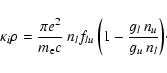
 enter through
 ,
given in
standard notation by
,
given in
standard notation by
 |
(6) |
 using the beam that leaves the photosphere with
 and assuming no limb-darkening.
As in Paper I, the data for the  105 lines contributing to are from Kurucz & Bell (1995). The fluxes are derived from the emergent fluxes of TLUSTY
models (Lanz & Hubeny 2003) by smoothing with a box filter of width
1000 km s-1. Photospheric line-blanketing is therefore included but
wind-blanketing is neglected.
105 lines contributing to are from Kurucz & Bell (1995). The fluxes are derived from the emergent fluxes of TLUSTY
models (Lanz & Hubeny 2003) by smoothing with a box filter of width
1000 km s-1. Photospheric line-blanketing is therefore included but
wind-blanketing is neglected.
The treatment of ionization and excitation is basically that of Abbott & Lucy (1985) as updated in Lucy (1999), with dilution as the dominant NLTE effect. Chemical composition is as stated in Sect. 2.1 of Paper I.
When derived as above,
 depends
only on the local properties of the wind at r, including the derivative
depends
only on the local properties of the wind at r, including the derivative
 .
But line formation is non-local, occurring over a
finite velocity interval corresponding to a few times the mean
thermal speed of the absorbing ions.
Accordingly,
.
But line formation is non-local, occurring over a
finite velocity interval corresponding to a few times the mean
thermal speed of the absorbing ions.
Accordingly,
 in Eq. (5) - the Sobolev
derivative - represents an average over this interval. As such, it does not
have the same standing as
in Eq. (2) - the Newtonian derivative.
in Eq. (5) - the Sobolev
derivative - represents an average over this interval. As such, it does not
have the same standing as
in Eq. (2) - the Newtonian derivative.
Though doubtless aware of this distinction, CAK nevertheless took the bold step
of assigning equal status to these two derivatives. In consequence,
the right-hand
side of Eq. (2) is a function of
,
which cannot then be
extracted algebraically.
When making an approximation, even if apparently well justified, we should be concerned whenever the mathematical nature of the problem changes, resulting in the addition or removal of crucial aspects of the solutions. The Sobolev approximation is certainly plausible for high velocity outflows and has been widely and usefully employed for transfer problems in stellar winds and supernovae. But when incorporated into the dynamical theory of winds via the CAK ansatz, a system of integro-differental equations is replaced by an ordinary differential equation (ODE). This results in the following changes to the solutions: 1) the sonic point is no longer a critical point; and 2) a new (CAK) critical point appears at supersonic velocities. Since critical points are certainly crucial, these changes should alert us to the possibility that the CAK solution may not be a good approximation to the corresponding solution of the basic integro-differential system. Despite this reservation, the above modified CAK theory is used in Sect. 3 to investgate supersonic winds.
Given the CAK ansatz, Eq. (2) reduces to a non-linear first order ODE with dependent variable v. Since the Sobolev approximation is not well justified in the sub- and transonic flow, an initial condition v = v1 at x = x1 is imposed at a point P1where the bulk motion is already highly supersonic. This point is selected from the appropriate RL of Paper I.
By thus choosing a supersonic matching point, we also avoid CAK theory's elimination of the sonic point as a critical point. Its correct role appears here implicitly via the initial condition derived from the RL, where regularity at the critical point v = a has already been imposed to determine J.
The mass-loss rate
is left as a free parameter
except when set
 ,
the rate predicted by the moving-RL.
,
the rate predicted by the moving-RL.
In this section, the topology of the solutions of the nonlinear ODE defined
in Sect. 2 is investigated. A general analytic discussion such as that of CAK
is not
possible because of the dropping of their simplifying assumptions.
Instead, the topology is investigated numerically but only along and
in the neighbourhood of the trajectories
 for specific models.
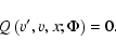
Following CAK, we write Eq. (2) formally as
 |
(7) |
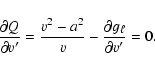 |
(8) |
For graphical presentation, it is convenient to make Q and
dimensionless by dividing by g*(r) and
 ,
respectively.
In addition, since
is constrained to be >0by the assumption of a monotonic velocity law (Sect. 2.2), we define
z to be the logarithm of the dimensionless
.
,
respectively.
In addition, since
is constrained to be >0by the assumption of a monotonic velocity law (Sect. 2.2), we define
z to be the logarithm of the dimensionless
.
Model S-30 of Pauldrach et al. (2001) is selected for detailed discussion.
The parameters are
 K,
K,
 ,
and
,
and
 ,
giving
,
giving
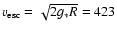 km s-1.
According to Paper I, for microturbulent velocity
 km s-1,
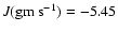 dex, corresponding to
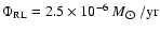 .
The initial condition
for the integration of Eq. (2) is obtained from the RL
at the point P1 where v = 3a. Thus
v1 = 52.5 km s-1and this occurs at
x1 = 0.950.
.
The initial condition
for the integration of Eq. (2) is obtained from the RL
at the point P1 where v = 3a. Thus
v1 = 52.5 km s-1and this occurs at
x1 = 0.950.
Because of the dependence of
on
,
specifying P1
does not uniquely determine the trajectory
for
x < x1 - i.e., the wind's velocity law.
This is illustrated in Fig. 1, which
plots the function Q1(z) obtained from Eq. (7) by setting
 .
We see that the equation Q1 = 0has two roots,
.
We see that the equation Q1 = 0has two roots,
 and
and
 ,
corresponding to rapid
and slow initial accelerations, respectively.
,
corresponding to rapid
and slow initial accelerations, respectively.
![\begin{figure}
\par\includegraphics[width=8cm]{8236fig1.ps}\par\end{figure}](/articles/aa/full/2007/42/aa8236-07/img50.gif) |
Figure 1:
Search for velocity gradient at P1 for model S-30
when
 .
The asterisks indicate the two roots of the equation Q1 = 0.
The open circle is the prediction
of the moving-RL from Paper I. .
The asterisks indicate the two roots of the equation Q1 = 0.
The open circle is the prediction
of the moving-RL from Paper I. |
| Open with DEXTER | |
Figure 2 shows how  and
and  vary with .
The roots
coalesce in a double root at
z*=0.78 when
vary with .
The roots
coalesce in a double root at
z*=0.78 when
 .
For
.
For
 ,
there is no root and so a matching supersonic solution does not then exist.
On the other hand, for
,
there is no root and so a matching supersonic solution does not then exist.
On the other hand, for
 ,
there are two
solutions given by the R- and S-branches. The appropriate continuation is
the one already
selected by the RL solution as it enters the Sobolev
regime. For the S-30 model in Paper I, the velocity derivative at
v = 3a gives
z1 = 1.42 for
,
there are two
solutions given by the R- and S-branches. The appropriate continuation is
the one already
selected by the RL solution as it enters the Sobolev
regime. For the S-30 model in Paper I, the velocity derivative at
v = 3a gives
z1 = 1.42 for
 dex, and this point is
plotted in Figs. 1 and 2. Clearly, the point on the R-branch is the
appropriate continuation.
dex, and this point is
plotted in Figs. 1 and 2. Clearly, the point on the R-branch is the
appropriate continuation.
![\begin{figure}
\par\includegraphics[width=8cm]{8236fig2.ps}\end{figure}](/articles/aa/full/2007/42/aa8236-07/img56.gif) |
Figure 2:
Velocity gradients satisfying the equation Q1 = 0 at P1as functions of .
The R- and S-branches are
indicated. The asterisks and the open circle are for
,
as in Fig. 1. The star on the S-branch is
the CAK solution. Points on the R-branch below the filled circle give
singularity-free winds extending to
. |
| Open with DEXTER | |
With the R-branch thus selected, Eq. (2) is integrated outwards from
P1 in order to determine
 .
As at P1, Eq. (7) continues to have two roots
and
until
.
As at P1, Eq. (7) continues to have two roots
and
until
 km s-1, at which point
 .
The steeper of the two possible velocity gradients is selected as the natural
continuation of the intial choice of .
The integration is continued to
.
The steeper of the two possible velocity gradients is selected as the natural
continuation of the intial choice of .
The integration is continued to
 ,
giving
a terminal velocity
,
giving
a terminal velocity
 km s-1. If the velocity law is
then fitted to the standard form
km s-1. If the velocity law is
then fitted to the standard form
 at
at
 ,
we obtain
,
we obtain
 .
These results are
unexceptional.
.
These results are
unexceptional.
But of exceptional interest is the integration's successful
continuation to
,
apparently without encountering a
singularity.
Because the root-finding uses Newton-Raphson (N-R)
iterations, a convergence failure would occur at a singularity, thus
terminating the integration at finite r.
In order to confirm that
does not cross
a locus of singular points, the nearest such points are now found.
When the integration reaches the point
 ,
the equation
,
the equation
 is solved for zi, thus determining
for the next
integration
step. But now z is varied away from zi in order to explore the solution
topology along the line
is solved for zi, thus determining
for the next
integration
step. But now z is varied away from zi in order to explore the solution
topology along the line
 in
in
 -space.
Thus we define a sequence of functions
-space.
Thus we define a sequence of functions
 of the single variable z, the first of which Q1(z) is already
plotted in Fig. 1.
of the single variable z, the first of which Q1(z) is already
plotted in Fig. 1.
In Fig. 3, this Qi-sequence is plotted for a dense set of points Pithrough the wind, and the stationary points zsi of the Qi are
marked. Since the curve defined by the zsi does not intersect the
line Q = 0, these calculations show that nowhere along the supersonic
wind is
 ,
thus confirming the absence of a
singularity and explaining the success of N-R iterations in
extracting
.
,
thus confirming the absence of a
singularity and explaining the success of N-R iterations in
extracting
.
![\begin{figure}
\par\includegraphics[width=8cm]{8236fig3.ps}\end{figure}](/articles/aa/full/2007/42/aa8236-07/img71.gif) |
Figure 3:
Functions Qi(z) for points
(vi, xi) throughout the
supersonic wind of model S-30. The asterisk is the initial gradient and the corresponding Q1(z) is labelled - see also Fig. 1. The arrows
indicate the direction of increasing v along the line Q = 0 and the filled
circles locate the stationary points zsi of the Qi(z). |
| Open with DEXTER | |
Sections 3.3 and 3.4 show that the moving-RL for S-30
can be matched to a singularity-free
wind extending to
.To explore how special such a continuation
is, a sequence of outward integrations from P1 is carried out with
as parameter. For each integration, the starting derivative
is the R-root from Fig. 2, and the integration continues with this root
as in Sect. 3.3. From this sequence, the singularity-free domain
is found to be
 .
This upper limit is indicated on the R-branch in Fig. 2. The corresponding
terminal velocity is
.
This upper limit is indicated on the R-branch in Fig. 2. The corresponding
terminal velocity is
 km s-1.
An integration with
increased to
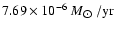 encounters a singularity when
v = 102.5 km s-1, at which point the N-R iterations fail
to converge. Interestingly, the proximity of a singularity is evident in the
successful integration for
encounters a singularity when
v = 102.5 km s-1, at which point the N-R iterations fail
to converge. Interestingly, the proximity of a singularity is evident in the
successful integration for
 in the form of a sharp decrease
in
in the form of a sharp decrease
in
 at
at
 km s-1.
Clearly,
km s-1.
Clearly,  is the value of
such that the
outward integration just grazes the locus of singular points. The velocity
of this tangent point for S-30 is
is the value of
such that the
outward integration just grazes the locus of singular points. The velocity
of this tangent point for S-30 is
 km s-1.
Because
comfortably exceeds
 ,
the successful continuation
of the RL is not fortuitous. Such continuations can
therefore be anticipated for RL's covering a wide range
of vt.
,
the successful continuation
of the RL is not fortuitous. Such continuations can
therefore be anticipated for RL's covering a wide range
of vt.
With radiative transfer treated using the Sobolev approximation, Abbott (1980)
studied the propagation of density fluctuations in line-driven winds. He
demonstrated that spherically-symmetric radiative-acoustic waves are non-
dispersive and propagate in the local matter frame with velocities
C+ and -C-, given by
 |
(9) |
 .
Transforming
to the star's frame, we see that information can propagate inwards towards
the star if u < 0, where
.
Transforming
to the star's frame, we see that information can propagate inwards towards
the star if u < 0, where
| u = v - C- . | (10) |
.
He thereby demonstated that
the CAK critical point is the furthest point downstream that can communicate
with and therefore influence every other point in the wind. This physical
interpretation of what had hitherto only had a mathematical justification
is undoubtedly a major reason for the almost universal acceptance of CAK
theory as
the correct theoretical foundation for line-driven winds and, in particular, of
the CAK critical point's role in determining .
Abbott's analysis can be applied to study information flow
in the singularity-free supersonic wind of S-30. Points in
the wind where u > 0 cannot communicate with the upstream flow.
From Eqs. (8)-(10), we find that
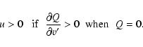 |
(11) |
 .
Thus no point in this solution can
influence the upstream structure by means of Abbott waves. In particular,
no information propagates back into the RL across the
boundary at x1.
.
Thus no point in this solution can
influence the upstream structure by means of Abbott waves. In particular,
no information propagates back into the RL across the
boundary at x1.
Figure 3 suffices for these qualitative remarks. The actual propagation speeds
are as follows: u=17.4 km s-1 at P1,
increases to a maximum of 705.2 km s-1 when
v = 1644 km s-1, then decreases to 620 km s-1 in the
terminal flow.
The propagation speeds are also of interest for the limiting singularity-free
solution with
(Sect. 3.5). Initially, u = 11.4 km s-1at P1, drops to a minimum of 0.8 km s-1at v = 104.5 km s-1, then rises monotonically to 217 km s-1in the terminal flow. This near approach to u = 0 reflects this solution's
close proximity to the singular locus when
km s-1.
The propagation criterion can also be applied to Figs. 1 and 2. The S-roots
of the equations
 are such that
 ,
so u < 0and information
can propagate back into the RL. The opposite holds for the R-roots.
When the roots coalesce, the double root is such that
,
so u < 0and information
can propagate back into the RL. The opposite holds for the R-roots.
When the roots coalesce, the double root is such that
 ,
whence
u = 0 and P1 is a singularity.
,
whence
u = 0 and P1 is a singularity.
As noted above, Abbott demonstrated that u changes sign at
 ,
the
velocity of the CAK critical
point, from being < 0 when
,
the
velocity of the CAK critical
point, from being < 0 when
 - i.e., in the upstream sub-critical
flow, to being
>0 when
- i.e., in the upstream sub-critical
flow, to being
>0 when
 - i.e., in the downstream super-critical flow.
Thus, the CAK solution constrained to pass through P1 must correspond to
a point on the S-branch of Fig. 2. Accordingly,
shooting integrations starting at P1 with the S-root
- i.e., in the downstream super-critical flow.
Thus, the CAK solution constrained to pass through P1 must correspond to
a point on the S-branch of Fig. 2. Accordingly,
shooting integrations starting at P1 with the S-root
 are used
as shown in Fig. 4 to
bracket the value of
are used
as shown in Fig. 4 to
bracket the value of
 .
To sufficient accuracy,
.
To sufficient accuracy,
 ,
and this is plotted on
the S-branch in Fig. 2.
,
and this is plotted on
the S-branch in Fig. 2.
This calculation shows that a CAK-continuation of the moving-RL fails on
two counts. Not only is
 as anticipated
in Sect. 1, but the respective solution branches also differ: the sub-critical
zones of CAK winds are on the S-branch, whereas the RL enters the
Sobolev regime on the R-branch.
as anticipated
in Sect. 1, but the respective solution branches also differ: the sub-critical
zones of CAK winds are on the S-branch, whereas the RL enters the
Sobolev regime on the R-branch.
![\begin{figure}
\par\includegraphics[width=8cm]{8236fig4.ps}\end{figure}](/articles/aa/full/2007/42/aa8236-07/img95.gif) |
Figure 4:
Shooting integrations to determine
,
all starting
at P1. The curves are labelled with
in units of
 . . |
| Open with DEXTER | |
The investigation of S-30 in Sect. 3 provides strong support for the approach
in Paper I - i.e, determining
J as an eigenvalue of the equations governing the structure of the
moving-RL, assuming no influence from the highly supersonic
exterior flow.
First, a singularity-free supersonic solution extending to
exists with
.
Second, this solution is everywhere super-critical in regard to Abbott waves,
which therefore carry no information back into the RL.
In order to demonstrate that this support is not restricted to S-30, identical
calculations are reported for the two other Pauldrach et al.
models considered in Paper I, namely D-40 and D-50. Numerical details for
all three models are given in Table 1. Velocities are in km s-1,
mass fluxes in gm s-1 and mass-loss rates in
 .
.
Table 1: O-star winds.
Some noteworthy aspects of Table 1 are as follows:
 for D-40 suggests that
is too low, but may also be a consequence of the no attenuation
assumption (Sect. 2.2) retained from CAK.
for D-40 suggests that
is too low, but may also be a consequence of the no attenuation
assumption (Sect. 2.2) retained from CAK.
 so that matching
singularity-free exterior solutions exist. Moreover, we can anticipate that
this remains true for the reduced
's corresponding to higher
so that matching
singularity-free exterior solutions exist. Moreover, we can anticipate that
this remains true for the reduced
's corresponding to higher
 's (see Table 1, Paper I).
and ,
we see that in each case the RL selects the R-root as the
appropriate continuation to highly supersonic velocities. The existence of
two barriers to matching onto a CAK exterior solution is therefore
further supported.
 .
This contrasts
dramatically with CAK's O5f model (similar to D-50) where the corresponding
last point
.
This contrasts
dramatically with CAK's O5f model (similar to D-50) where the corresponding
last point
 is at
is at
 km s-1, a velocity well
in excess of
km s-1, a velocity well
in excess of
 .
Accordingly, no matter moving with
.
Accordingly, no matter moving with
 is out of contact with
the upstream flow, suggesting perhaps a mechanism that adjusts the
wind's base structure to ensure eventual escape.
But this possibly appealing aspect of the original CAK theory
does not survive subsequent modifications, especially those of Pauldrach et al.
(1986) - see their Table 1 and Fig. 2a.
is out of contact with
the upstream flow, suggesting perhaps a mechanism that adjusts the
wind's base structure to ensure eventual escape.
But this possibly appealing aspect of the original CAK theory
does not survive subsequent modifications, especially those of Pauldrach et al.
(1986) - see their Table 1 and Fig. 2a.
 ,
the ratio of dilution
factor to electron density, the ionization balance throughout these winds
is such that matter remains an efficient scatterer of
UV radiation, and Doppler shifts continually irradiate lines with fresh
unattenuated continuum.
,
the ratio of dilution
factor to electron density, the ionization balance throughout these winds
is such that matter remains an efficient scatterer of
UV radiation, and Doppler shifts continually irradiate lines with fresh
unattenuated continuum.
The aim of this paper has been to investigate the problem of matching
the moving-RL's of Paper I to supersonic winds extending to
.
Perhaps surprisingly, matching exterior solutions have been obtained with a
modified CAK procedure using
the Sobolev approximation. But in contrast to standard CAK theory,
the entire solution thus constructed has the same critical-point
structure as the basic integro-differential system. Thus the sonic point
retains its role as a critical point (Paper I), and a CAK critical point no
longer
appears in the supersonic flow (Sect. 3.5). In consequence, there is a
reasonable
expectation that such solutions will be good approximations to solutions
obtained with non-Sobolev transfer (Sect. 2.3).
Use of a modified CAK procedure
for the exterior solutions has allowed comparisons
with CAK solution topology and, crucially, with Abbott's discussion of
information propagation by radiative-acoustic waves. With these issues now
clarified, future calculations should re-introduce multi-line scattering.
This can be done by extending the Monte Carlo procedures of Paper I to
- see also Abbott & Lucy (1985) and Vink et al. (2000). Another
attractive possibility is to revive the comoving frame approach
(Mihalas et al. 1975;
Weber 1981; Pauldrach et al. 1986). In either case,
is determined
by the constraint of regularity at the sonic point and not at the CAK
critical point, which no longer exists.
Accordingly, scaling relations for
need to be re-investigated
since the basis is undermined for those obtained from the CAK critical point.
Acknowledgements
The referee, S.P. Owocki, is thanked for his comments and suggestions. This investigation also benefited from points raised by J. Puls in his report on Paper I.