A&A 471, 993-997 (2007)
DOI: 10.1051/0004-6361:20066809
C. Dauphin
LUTh, Observatoire de Paris, 92195 Meudon Cedex, France
Received 24 November 2006 / Accepted 21 May 2007
Abstract
Context. Particles accelerated in solar flares draw their energy from the magnetic field. The dissipative scale of the magnetic energy in the solar corona implies that the magnetic energy is transmitted to the particles through a large number of dissipative regions (DR).
Aims. To finally compute the particle energy distribution, we present an approach to linking the magnetic energy release to the acceleration process that occurs in each DR .
Methods. Although not directly observed, the magnetic energy release process is assumed to evolve in an SOC state that leads to the power-law behaviour of the probability distribution function for the energy released in each DR. We consider that most of the accelerated particles leave the acceleration region after one interaction, but we introduce a distribution of the particle acceleration lengths inside each acceleration region.
Results. We calculate the kinetic energy distribution of the accelerated particles. Our model allows us to identify the physical process that determines each part of the particle energy distribution.
Conclusions. As a conclusion, we discuss the limitations of the approach presented in this paper.
Key words: Sun: flares - acceleration of particles
A solar flare is defined as a sudden transfer of magnetic energy to the ambient coronal plasma that leads to heating, flows, and particle acceleration. Observations and analyses of hard X-ray emissions are the most direct diagnostic of these non thermal particles. The last decades of observations have shown that a large number of particles are accelerated (![]() 1038 electrons s-1) to energy going up to several MeV, which implies a high efficiency for the acceleration mechanism.
1038 electrons s-1) to energy going up to several MeV, which implies a high efficiency for the acceleration mechanism.
One of the most relevant pieces of information that allows us to constrain the physical process that occurs during particle acceleration is certainly provided by the particle energy spectrum. Generally, hard X-ray spectra are reproduced by a simple or a double power-law electron spectrum (Holman et al. 2003; Conway et al. 2003; Piana et al. 2003). These electron spectra show a steep break generally between 10 keV and 100 keV, and the spectral index below the break is usually lower than the spectral index at higher energy (Lin et al. 1982).
In this paper, an attempt is made to identify the physical processes that determines each part of the particle energy distribution. The basic idea is to take the particle acceleration process and the magnetic energy release process into account.
Particle acceleration mechanisms can be divided into three different classes: shock acceleration, turbulent acceleration, and direct electric field (further discussion can be found in the review of Miller et al. 1997). The energy of all aspects of the flare process, including particle acceleration, must ultimately come from the release of the stored magnetic energy. One possible way to release the magnetic energy stored in the corona is the formation of small-scale magnetic discontinuities where the frozen-in law is violated and where instabilities and anomalous resistivity can easily rise. Here, we consider that the particles are accelerated by the direct electric field that appears in such a region.
A large number of works have been devoted to analytical and numerical analyses of particle acceleration by a direct electric field in X-point (e.g. Hamilton et al. 2005), by a reconnecting current sheet (Litvinenko 1996; Zharkova & Gordovskyy 2004; Wood & Neukirch 2005), and in a spin and fan geometry (Litvinenko 2006; Dalla & Browning 2005, 2006). These different studies usually found a power-law particle-energy distribution due to the configuration of the magnetic field that generates a chaotic behaviour of the particle trajectories.
The complex magnetic environment of an active region (Arzner & Vlahos 2006), as well as the turbulent nature of photospheric motions that externally and continuously drives the system, will add new stresses to the existing large-scale topologies and lead to the formation of short-lived, small-scale magnetic discontinuities (see e.g., Vlahos et al. 2004; Fragos et al. 2004). Moreover, the properties of coronal turbulence implies that the magnetic energy is dissipated and transmitted to the particles on very small lengthscales (Einaudi & Velli 1994). Thus, every model of particle acceleration during a solar flare has to take into account the large-scale physical process that leads to the appearance of several dissipative regions where the particle acceleration process can takes place.
The idea of multiple dissipation sites in flares has been modelled by Lu & Hamilton (1991) by using the self-organised criticality (SOC) concept. Evolution of this model followed by satisfying the Maxwell's equations (e.g. Vlahos et al. 1995; Vassiliadis et al. 1998; Isliker et al. 2000). These SOC and associated cellular automata models identify dissipation occurring in many spatially separated regions. Several authors have investigated the problem of particle acceleration by using a model in which the accelerated particles move between the dissipation regions (Vlahos et al. 2004; Anastasiadis et al. 2004; Dauphin et al. 2007). Particles gain or lose energy in each dissipative region. The rate of energy change is proportional to the electric field, which is a function of the magnetic energy.
Another approach is to calculate the acceleration of particles in an electromagnetic field taken from MHD simulation or random-phase turbulence proxies or p-model (Decamp & Malara 2006). To study particle acceleration, the electromagnetic field is frozen in time, and test particles are injected into the simulation box. The energy gain of the test particles is calculated by solving the relativistic equations of motion. Such an approach has been used by Dmitruk et al. (2004, 2005) in direct simulations of homogeneous 3D MHD turbulence and by Arzner & Vlahos (2004) and Arzner et al. (2006), who have worked with random-phase turbulence proxies. Recently Onofri et al. (2006) addressed the problem of stochastic acceleration in turbulent electric field generated by 3D reconnection and Turkmani et al. (2005, 2006) addressed the issue of particle acceleration in a 3D coronal MHD model. Some particles undergo rapid and systematic energy gain and leave the computational box with relastivistic energy, whereas other particles do not intereact with the current sheets and gain no energy or little.
These different studies cannot simultaneously take into account the process that leads to the appearance of the acceleration regions and the particle acceleration process inside each of these regions. In this paper, we consider these processes by introducing two probability distribution functions that represent the spatial distribution of acceleration regions and the distribution of the particle acceleration lengths inside each acceleration region.
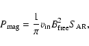
![\begin{figure}
\includegraphics[width=11.5cm,height=8cm]{6809fig1.eps}\end{figure}](/articles/aa/full/2007/33/aa6809-06/img6.gif) |
Figure 1: Schematic view of a global acceleration region composed of multiple acceleration regions. The size of one AR is proportional to the value of the magnetic energy coming into the acceleration region. The small grey arrows represent the direction of accelerated electrons in each AR. The grey and white arrows outside the global acceleration region represent, respectively, the accelerated electrons and ions. |
| Open with DEXTER | |
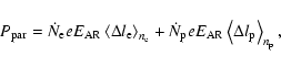
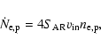
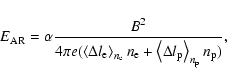
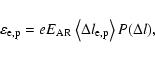
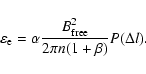
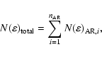
We consider an isolated acceleration region (AR). Particles are accelerated by the electric field into the AR and gain energy from the magnetic energy. We equate the magnetic energy flux to the particle energy flux in order to determine the electric field into the acceleration region.
The magnetic energy flux is given by the equation:
 |
(1) |
 |
(2) |
 |
(3) |
 |
(4) |
 |
(5) |
 |
(6) |
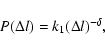
We assume that the probability distribution function of the acceleration length is given by
 |
(7) |
 |
(8) |
 |
(9) |
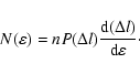
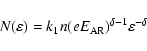
We now consider several DR leading to a "gas'' of acceleration regions with different values of magnetic energy incoming into each AR. Figure 1 shows a schematic view of a global acceleration region (GAR) composed of multiple acceleration regions. Particles (electrons and ions) are accelerated in a different direction into each AR. Thus, electrons and ions are accelerated in the same direction outside of the global acceleration region. The total particle energy distribution outside of the global acceleration region corresponds to the sum of the particle energy distribution in each AR. In other words, every particle interacts only with one acceleration region.
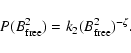
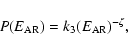
We consider that the probability distribution function of the magnetic energy entering into the different AR is given by a power law (Vlahos et al. 2004, and references therein):
 |
(10) |
 |
(11) |
 |
(12) |
We compute the total particle energy distribution given by Eq. (12) for different values of
![]() .
For each AR, we randomly select
.
For each AR, we randomly select ![]() between 0 and 1. Particles are injected into the acceleration volume with an initial Maxwellian distribution with a temperature of 106 K and with initial velocities in the range
between 0 and 1. Particles are injected into the acceleration volume with an initial Maxwellian distribution with a temperature of 106 K and with initial velocities in the range
![]() where
where
![]() is the thermal velocity. The particle energy distribution for electrons and ions is calculated with a density of
is the thermal velocity. The particle energy distribution for electrons and ions is calculated with a density of
![]() .
We consider only super Dreicer events, thereby normalizing the minimal value of the electric field distribution to the Driecer electric field equal to
.
We consider only super Dreicer events, thereby normalizing the minimal value of the electric field distribution to the Driecer electric field equal to
![]() .
.
We consider an example of particle acceleration from 10 000 AR. The electric field value of each AR is simulated between ED and 105 ED with a spectral index equal to 1.6 (Vlahos et al. 1995). As an example, the particle's acceleration length values are included between ![]() 0.5 km and
0.5 km and ![]() 16 km with a spectral index equal to 3.
16 km with a spectral index equal to 3.
![\begin{figure}
\par\includegraphics[width=7cm,height=6.5cm]{6809fig2.eps}\end{figure}](/articles/aa/full/2007/33/aa6809-06/img43.gif) |
Figure 2:
Kinetic particle energy distribution obtained for
|
| Open with DEXTER | |
![\begin{figure}
\par\includegraphics[width=14cm,height=7cm]{6809fig3.eps}\end{figure}](/articles/aa/full/2007/33/aa6809-06/img44.gif) |
Figure 3:
Kinetic particle energy distributions obtained for
|
| Open with DEXTER | |
Figure 2 shows the particle energy distribution obtained from these 10 000 AR. Several results can be drawn from this figure:
| (13) |
Finally, we have to underline, in the case of one interaction for each particle, that the values of the spectral index below and above the break corresponds, respectively, to the spectral index value chosen for the probability distribution of the magnetic energy release and particle acceleration length.
The parameters ![]() and
and
![]() determine the acceleration process of electrons and ions inside each acceleration region. Thus, the total ion energy distribution depends on the values of the two parameters. Although the exact determination of
determine the acceleration process of electrons and ions inside each acceleration region. Thus, the total ion energy distribution depends on the values of the two parameters. Although the exact determination of ![]() and
and
![]() for electrons and ions is beyond the scope of this paper, we can discuss the effect of these two parameters on the ion energy distribution. The parameter
for electrons and ions is beyond the scope of this paper, we can discuss the effect of these two parameters on the ion energy distribution. The parameter ![]() models the possibility that electrons and ions are accelerated at different energies inside each acceleration region. Compared to the kinetic energy distribution of electrons, this parameter changes the value of the maximum energy gained by the ions and changes the value of the break in the ion energy distribution. The probability distribution function
models the possibility that electrons and ions are accelerated at different energies inside each acceleration region. Compared to the kinetic energy distribution of electrons, this parameter changes the value of the maximum energy gained by the ions and changes the value of the break in the ion energy distribution. The probability distribution function
![]() changes the particle energy distribution above the break.
changes the particle energy distribution above the break.
We now consider that some of the accelerated particles undergo multiple interactions. Moreover, we consider that the interaction of an accelerated particle with an acceleration region leads to a loss or a gain in energy for the particle. Thus, the amount of energy transmitted to a given accelerated particle during its interaction with an acceleration region is given by
 |
(14) |
Figure 3 shows the particle energy distribution obtained with 10% of the total number of particles that undergo several interactions. The distribution of the particle energy gain can be divided into four parts. The first one is the thermal plasma. The second part of the spectrum is due to the magnetic energy release process. The third part of the spectrum is due to the particle acceleration process in each acceleration region. The last part of the spectrum is created by the particles that undergo several interactions.Two comments can be drawn from this figure:
We have presented an acceleration model that assumes the acceleration of particles drawing their energy from the magnetic energy release in several dissipative regions. We consider that each dissipative region transmits a different amount of magnetic energy to the particles. Into each dissipative region, each particle has a different acceleration length that leads to a different energy gain. Thus, the small-scale physical processes that occur in acceleration regions are taken into account by introducing a distribution of the particles acceleration length inside each acceleration region.
In this model, the probability distribution function of the magnetic energy release is modelled by a power law. Furthermore, numerous acceleration models with various acceleration mechanisms (direct electric field in different magnetic field configurations) simulate the particle acceleration process in a single acceleration region (Dalla & Browning 2005; Wood & Neukirch 2004, 2005; Zharkova & Gordovskyy 2004, 2005a). The results of these models support our assumption of a probability distribution function of the particle acceleration length given by a power law. Moreover, we consider that the probability function of the particle acceleration length and of the magnetic energy release are independent (i.e. the particle acceleraton length is independent of the magnitude of the electric field).
One of the new assumptions introduced in this paper is that most of the particles are accelerated one time. We use this model to compute the total particle energy distribution. Several results can be drawn from this distribution:
In conclusion, we note that this model allows us to identify the physical processes that lead to the formation of the different parts of the particle energy distribution deduced from the observations. Such a particle acceleration mechanism can explain the main part of the energy distribution of the accelerated particles. However, other particle acceleration mechanisms, as acceleration by waves (Miller & Roberts 1995), are certainly acting during a solar flare. The relative importance of each mechanism as a function of the particle energy has to be investigated further.
Acknowledgements
The author would like to thank L. Vlahos for helpful comments.