A&A 471, 687-694 (2007)
DOI: 10.1051/0004-6361:20066491

Tracking granules on the Sun's surface and reconstructing velocity fields

I. The CST algorithm

M. Rieutord¹ - T. Roudier² - S. Roques¹ - C. Ducottet³

1 - Laboratoire d'Astrophysique de Toulouse et Tarbes, UMR 5572, CNRS et Université Paul Sabatier, 14 avenue E. Belin, 31400 Toulouse, France
2 - Laboratoire d'Astrophysique de Toulouse et Tarbes, UMR 5572, CNRS et Université Paul Sabatier, 57 avenue d'Azereix, BP 826, 65008 Tarbes Cedex, France
3 - aboratoire Hubert Curien, UMR5516, CNRS et Université Jean Monnet, 18 rue du Prof. B. Lauras, 42000 Saint-Étienne, France

Received 2 October 2006 / Accepted 12 April 2007

Abstract
Aims. Determination of horizontal velocity fields on the solar surface is crucial for understanding the dynamics of structures like mesogranulation or supergranulation or simply the distribution of magnetic fields.
Methods. We pursue here the development of a method called CST for coherent structure tracking, which determines the horizontal motion of granules in the field of view.
Results. We first devise a generalization of Strous method for the segmentation of images and show that when segmentation follows the shape of granules more closely, granule tracking is less effective for large granules because of increased sensitivity to granule fragmentation. We then introduce the multi-resolution analysis on the velocity field, based on Daubechies wavelets, which provides a view of this field on different scales. An algorithm for computing the field derivatives, like the horizontal divergence and the vertical vorticity, is also devised. The effects from the lack of data or from terrestrial atmospheric distortion of the images are also briefly discussed.

Key words: convection - turbulence - Sun: granulation - Sun: photosphere

1 Introduction

Determining the flows on the surface of the Sun has triggered many efforts over the last decade. Of special concern was determination of granules motions that can reveal horizontal flows on scales larger than, typically, twice their horizontal size $\sim$2000 km. This scale is small enough to provide observers of the Sun's surface with a detailed sampling of the large-scale flows, such as supergranulation, and therefore makes it very interesting to determine granule motions.

However, from the viewpoint of fluid mechanics, granules are not passive scalars whose motions trace that of the fluid; rather, they are structures in intensity or, assuming perfect correlation with temperature, coherent structures of temperature. But the evolution of the temperature field is the result of radiative, as well as advective, processes. It is only in case that the latter dominates that the motions of granule can be associated with horizontal flows. Using numerical simulations in a large horizontal box, we have shown that granule motions are highly correlated with horizontal flows when the scale is larger than $\sim$2500 km (Rieutord et al. 2001); below this scale, granule motions should be considered as (solar) turbulent noise.

Once the equivalence of plasma motion and granule motion is assumed, one is left with the problem of measuring the latter motion. This is not an easy task owing to the small angular size ($\sim$1.3 $^{\prime\prime}$) of the structures. Ground-based observations are sensitive to atmospheric turbulence, while space observations are expensive owing to the (relatively) large aperture needed for resolving granules.

Basically, two techniques have been used to measure horizontal velocity fields: either the tracking of individual granules (Strous 1995) or local correlation tracking (November & Simon 1988). The results of these two techniques have been compared (Roudier et al. 1999; Simon et al. 1995) and found to broadly agree; in the test using numerical simulations (Rieutord et al. 2001), they show the same degree of correlation with the actual plasma flows. However, detailed examinations (Roudier et al. 1999; Simon et al. 1995) have demonstrated worrying differences, especially when field derivatives like vertical vorticity and divergence are computed.

In fact from the point of view of signal processing, these two methods differ fundamentally. On the one hand, granule tracking emphasises the importance of the granule, gives no signal in between granules, and yields a velocity field that is sampled randomly following the distribution of granules. On the other hand, local correlation tracking (LCT hereafter) treats granules and intergranules on an equal footing and yields a velocity field on a regular grid. Broadly speaking, the two methods differ in the interpolation process, which unfortunately influences the final result.

In this paper we present and analyse in some detail an algorithm based on granule tracking which is able to give a reconstruction of the velocity field at all scales larger than the sampling scale. This algorithm has already been introduced in Roudier et al. (1999) in a preliminary version. We call it CST for coherent structure tracking to underline its relation with the physics lying behind it. Such an algorithm is close in its principles to particle-imaging velocimetry (PIV), as used in experimental fluid mechanics (e.g. Adrian 2005).

We developed this algorithm for three reasons: the first is obviously because it gives a different view of the data than does the LCT algorithm, since many interpolation problems may influence the final results (see the discussion in Potts et al. 2003). The second one is that it may be used on raw data and gives an estimate of the error introduced by atmospheric distortion (see the companion paper, Tkaczuk et al. 2007, in which this point is developed). Finally, it offers the possibility of selecting specific structures according to their nature, size, lifetime, etc. and of studying their motion.

In the next section we discuss the different steps of the algorithm, especially the segmentation and interpolation processes, and also point out the effects of regions lacking data. Discussion and conclusions follow.

2 The CST algorithm

Before describing the different steps in some detail, let us recall the five main steps of this algorithm:

• segmentation of the image and granule identification;
• measurement of velocities at granule locations;
• reconstruction of the velocity field;
• calculation of field derivatives (like the z-component of the vorticity and divergence);
• estimation of the noise.

We now go into detail for each one in turn.

2.1 Segmentation and granule identification

To identify a granule one needs a criterion with which to decide whether a given pixel belongs to a given structure or not. This criterion needs to be local in order to avoid threshold effects due to large-scale variations in intensity, which either come from terrestrial atmospheric effects, solar acoustic waves, or even magnetic fields.

A classical criterion is based on detecting local maxima of the intensity through the curvature C=I_i+1-I_i-(I_i-I_i-1)(Roudier et al. 1999; Strous 1995). This criterion has the advantage of being simple, robust, and therefore quite efficient. However, comparing the detected patterns with the original image shows that this criterion underestimates the size of the granules. It is therefore interesting to know whether this criterion can be improved. An objective test of this improvement will be that the lifetime of the granules is increased.

	Figure 1: Comparison of the result of different segmentations on the same test image. From top to bottom and left to right we have : the original image, the result of Strous's method, the result of the BW method, the result of the proposed method. Note that BW leaves some granules undetected.
Open with DEXTER

Another method has been proposed by Bovelet & Wiehr (2001, hereafter referred to as BW), with a multiple-level tracking algorithm. It is based on the use of multiple-threshold levels applied to the intensity image. The granules detected at a high level are gradually extended to adjacent pixels whose intensity exceeds the lower level, while keeping a minimum distance with respect to other granules. This approach, which is very similar to a watershed-based segmentation (Soille 1999; Vincent & Soille 1991), yields sizes and shapes of granules that conform more to direct observation of the image. Nevertheless, the number of detected granules is less compared to the Strous algorithm because this method is based on the intensity.

The Strous-curvature criterion is more efficient at separating the granules. It consists in selecting the pixels whose local minimal curvature is not negative. This curvature is calculated in the four directions defined by the 8 neighbours of the considered pixel. The underestimation of the granule size stems from real granule's extension being greater than the positive curvature region. We thus propose a new segmentation algorithm (hereafter termed CD) that combines both ideas of BW and the Strous algorithm. It consists in the following steps:

• Calculation of the "minimal curvature image'' : for each pixel, the minimal curvature among the four directions is computed.
• Detection of the granules as non negative curvature pixels in the minimal curvature image.
• Extension of the detected granules with points whose minimal curvature value is greater than a given (negative) threshold $t_{\rm ext}$, while keeping a minimal distance of one pixel between each pair of granules.

The last step can be reached using the watershed algorithm on the minimal curvature image, with an additional condition requiring that the curvature remains above $t_{\rm ext}$.

	Figure 2: Comparison of the effect of different segmentations on lifetimes of granules. BW refers to the Bovelet and Wiehr method while CD refers to our method (see text); the associated number is the extension threshold parameter $t_{\rm ext}$.
Open with DEXTER

This new approach leads to a segmentation with the same granules as Strous's approach, but with a controllable size. Strous's segmentation is obtained with $t_{\rm ext}=0$. Decreasing the value of $t_{\rm ext}$ extends the granules. In Fig. 1 we illustrate the discussed segmentation method using Pic-du-Midi data. This figure illustrates the way our segmentation extends that of Strous and closely follows the shape of granules.

To study the influence of the segmentation on the lifetime of granules, we plotted the statistic of the lifetime for the three methods : the Strous method, BW method, and our proposed method. For our method, we took three different threshold values: $t_{\rm ext}=0$, $t_{\rm ext}=-0.1$, and $t_{\rm ext}=-0.3$ (Fig. 2).

This figure shows that, broadly speaking, the segmentation does not influence the statistics of lifetimes very strongly. However, some differences can be noticed in the detail. The BW algorithm, by detecting less granules, shows a deficit of short-lived and long-lived granules; on the other hand, our algorithm eliminates long-lived structures when used with too low a threshold. We understand this behaviour as the result of enhanced splitting of larger structures.

In conclusion, Strous's algorithm seems the most efficient for our purpose, and it can be improved in the way we described, but at the price of increasing the computation effort a lot.

Once the image has been segmented, each granule needs to be identified. This operation, although very simple, can be quite time-consuming since all pixels should be tested at least once. The most efficient way we have found to deal with this operation is to use a recursive algorithm, letting granules grow from a single pixel. A pixel belongs to a granule if it shares at least one side with another pixel of the granule.

	Figure 3: Trajectories of granules in a five-minute time sequence. Top: Granule displacements in a small subfield. Bottom: enlarged view of a granule trajectory. Data are from the 1988 Pic-du-Midi series (e.g. Muller et al. 1992).
Open with DEXTER

  
2.2 Measuring the velocities

Once the granules have been identified, the (x,y) coordinates of their barycentre are computed. Hence, each image is converted into a set of points $\vX_{i,n}$ describing the position of the granules at time t_n. These data may be completed by the set of granules surfaces, shapes, etc.

The set of points $\{\vX_{i,n}\}$ is then divided into trajectories

$$\left\{ \vX_{i(k),n}\right\}_{n_i \leq n\leq n_\ell}.$$

This notation means that granules of index i(k) are in fact the same granule as the one that follows the kth trajectory; it appears at time t(n_i) and disappears at time $t(n_\ell)$.

Trajectories are identified by comparing each position $\vX_i$ on two consecutive images and putting nearest neighbours together provided their position does not differ more than a given threshold that is determined by an upper bound on the velocity. Typically, we reject velocities higher than 5 km s^-1.

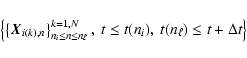
If one disposes of a long time series of images, it may be useful to determine the time evolution of the velocity field. For this purpose a time window of width $\Delta t$ needs to be used and trajectories are restricted to time windows. Hence, for a given time window, one derives a set of N trajectories:

$$\left\{ \left\{ \vX_{i(k),n}\right\}_{n_i \leq n\leq n_\ell}^{k=1,N}, ~ t\leq t(n_i),~ t(n_\ell)\leq t+\Delta t\right\}$$

existing in the field during the time $[t,t+\Delta t]$. We show an example of such a set of trajectories in Fig. 3. We clearly see from the enlarged view that granule motion is dominated by an erratic motion that mixes (Earth) atmospheric noise with the turbulent random flow of solar convection.

From this set we derive a mean velocity associated with each trajectory; the kth trajectory gives the velocity

$$\left\langle \vec{V}_k\right\rangle = \frac{\vX_{i(k),n_2} - \vX_{i(k),n_1}}{t(n_2)-t(n_1)},$$

which we associate with the mean position of the trajectory

$$\vX_k = \frac{1}{n_2-n_1+1}\sum_{n=n_1}^{n_2}\vX_{i(k),n}.$$

Hence we end up with the set

$$\left\{\vec{V}_k, \vX_k\right\}_{k=1,N}$$

which describes the velocity field during the time interval $[t,t+\Delta t]$.

The values of the velocities are of course not uniformly distributed in the field of view and we need to know how they constrain the velocity field at a given resolution: small-scale components are weakly constrained, while large-scale ones are highly constrained. The maximum resolution for the velocity field is given by the density of trajectories and can be estimated by the mean distance $\langle d\rangle$ between the $\vX_k$. As the time window $\Delta t$ is increased, the maximum resolution increases according to the law $\langle d\rangle \propto 1/\!\sqrt{\Delta t}$ as clearly shown by Fig. 4. This law arises because granules cover the Sun's surface permanently. From it, we can derive the maximal spatial resolution for a given time resolution. Indeed, from Fig. 4, it turns out that the mean volume of space-time occupied by one granule is $\sim$1200 Mm² s.

	Figure 4: Mean distance between velocity vectors as a function of the time window used for the measurement. The line shows the law $\langle d\rangle \propto 1/\!\sqrt{\Delta t}$.
Open with DEXTER

This value is useful for determining the highest time resolution that can be allowed for the large-scale velocity fields. Indeed, as pointed out in Rieutord et al. (2001), granules cannot be used to trace plasma flow under a scale of 2.5 Mm (except in the case of very rapid flows like "explosion'' of granules); thus the determination of a large-scale flow needs a mesh size not smaller than 1.25 Mm. This means that each grid point will have a have a trajectory only if $\Delta t \geq 768$ s. Conservatively, we estimate that the time resolution cannot be higher than 15 min.

Often time resolution is not needed and therefore $\Delta t$ is much larger than 15 min. In such a case, several velocities may be given by granules appearing at a given place on the grid. We then use the average velocity of the granules as the measure of the local velocity. This introduces another quantity, namely the rms fluctuation around this mean. This rms velocity is a measure of the proper velocity of granules and therefore a proxy of the local strength of turbulent convection.

2.3 Derivation of the velocity field by MRA

Figure 5: Isoline plot for the z-component of the curl of the velocity field vx=-y, vy=x with some values of $\vec{v}$ randomly set to zero (black dots in the field). To the left, the scaling function $_4\phi$ of Daubechies wavelet is used; to the right we use $_8\phi$. The main difference between these two wavelets is the width of their support, twice larger on the right. Note the border effects in both figures as well as the patterns introduced by the absence of data and their dependence on the support of the wavelet. The large blank areas are at the constant value of 2, as expected; solid lines represent isolines of a value different from 2 and dotted lines show negative value isolines. X and Y units are grid points.

Open with DEXTER

	Figure 6: To the left, the velocity field with a small mesh size (713 km) is complete with 83% of data, while on the right, using a larger mesh size of 1223 km, the velocity field is complete to 99%. Patterns of velocities are easily identified between the two. We used a time interval of 15 min.
Open with DEXTER

Once the velocities in the field of view are determined, we need to know what kind of flow they represent: for instance, vortices, shear layers, diverging sources, etc. For this purpose we need to determine the best continuous differentiable field that approximates the data. The determination of such a field can be done in various ways, but we wish to introduce no information or a minimum of into this process. We also wish to avoid the propagation of errors and noise in the field of view.

We have found that wavelet multi-resolution analysis (MRA) is an interesting tool for this purpose, because it gives a decomposition of the signal at all the scales allowed by the size of the box and therefore gives a good view of all the components of the signal (Meyer 1987; Mallat 1989).

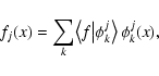
The basic idea of a "multi-resolution representation'' of  $L^2({\rm I\!R})$is to project a signal f on a "wavelet orthonormal basis'' of $L^2({\rm I\!R})$, at which point it is possible to extract the "difference in information'' between two successive approximations of the signal (approximations at the resolution 2^j and 2^j+1). The wavelet orthonormal basis is a family of functions $\sqrt{2^j}\psi(2^jx-k)_{j,k\in {{\mathchoice {\hbox{$\sf\textstyle Z\kern-0.4em... ...ptstyle Z\kern-0.3em Z$ }} {\hbox{$\sf\scriptscriptstyle Z\kern-0.2em Z$ }}}}}$ built by dilations and translations of a unique function $\psi(x)$: the analysing wavelet. The decomposition thus obtained is this MRA. The signal can be reconstructed from this representation without any difficulty. We give a minimal background to this technique in appendix A.

Figure 7: Divergence of the velocity field shown in Fig. 6. As in Fig. 6, on the left we have the more resolved, but less complete, sample and on the right the less-resolved, but more complete, sample. In the first row the data have been only slightly filtered (they are projected on the space j=1), and one can hardly identify any common structure in the two plots. However, we clearly see some common features between the two plots when considering the low frequency j=3-component.

Open with DEXTER

Now we need to specify the choice of the analysing wavelet. As in many problems of image processing, we choose the Daubechies wavelet because of its compact support. This property is important since it minimizes border effects and interactions between patterns of the signal during the filtering process. Moreover, using these wavelets also preserves the location of zero-crossing and maxima of the signal during the analysis, a property that results in mutual suppressive interactions across its different scale representations and superior robustness in noisy environments (Sahiner & Yagle 1993). Thus, the contours of the image can be determined efficiently. We understand that this property is important in image processing since the features of the image are preserved after filtering. For the velocity fields we are dealing with, this is also an interesting point, because we wish to identify flow structures like divergences and vortices.

Finally, wavelet analysis also allows us to determine the relevance (or the reality) of flow structures on different scales. One may indeed apply the MRA to the velocity field and the noise field. Then, for each scale of the flow, we can compare the details and the amount of noise to see whether the details are relevant or are simply noise structures.

2.4 Curl and divergence fields

Once an approximation of the velocity field is known, it is useful to detect flow patterns that may be important for the dynamics of the fluid. As the (measured) velocity field is purely two-dimensional, two quantities are relevant for enhancing flow structures: the divergence $D=\partial_xv_x+\partial_yv_y$ and the z-component of the vorticity $\zeta=\partial_xv_y-\partial_yv_x$.

The way derivatives can be computed can be explained with a one-dimensional example. Let us consider the approximation on scale jof the signal f

$$f_j(x) = \sum_k \bigl\langle f\bigr\vert \phi_k^j \bigr\rangle\, \phi_k^j(x),$$ (1)

where k represents the position of the wavelet. Differentiating this expression yields

$$\frac{{\rm d} f_j}{{\rm d}x} = \sum_k \bigl\langle f\bigr\vert \phi_k^j \bigr\rangle\, \frac{{\rm d} \phi_k^j}{{\rm d}x}\cdot$$

In the Galerkin method, this formula would be sufficient; however, in MRA the derivative of a function approximated with some resolution has meaning only in the same functional space, that is, with the same resolution. Therefore, ${\rm d}f_j/{\rm d}x$ also needs to be projected onto that space. Thus we are interested in

$$\Bigl\langle \phi_n^j\Bigr\vert \frac{{\rm d} \phi_k^j}{{\rm d}x} \Bigr\rangle\,\cdot$$

It therefore turns out that the discrete approximation of the derivatives can be easily derived from that of the original functions by a simple matrix multiplication. If $S_k^j=\bigl\langle f\bigr\vert \phi_k^j \bigr\rangle\,$ is the discrete approximation of f on scale j and S'^j_k the discrete approximation of ${\rm d}f/{\rm d}x$ on the same scale, then it follows that

$$S'^j_k = 2^{-j}\sum_l r_{k-l} S^j_l,$$ (2)

where

$$r_l = \int_{-\infty}^{+\infty} \phi(x-l)\frac{{\rm d} \phi}{{\rm d}x}{\rm d}x .$$

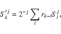These numbers can be computed through an algorithm described in Beylkin (1992).

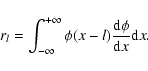
We show the computations of the curl field on a simple given velocity field in Fig. 5, namely v_x=-y, v_y=x. We see that, except for the border effects due to the finite size of the filter, value 2 is correctly restored.

2.5 The role of "holes''

One of the problems arising when reconstructing the velocity field comes from the presence of bins without data. Such bins produce structures in the divergence and curl fields. A simple illustration of the effect is given in Fig. 5 where the curl of a solid rotation velocity field is plotted. This figure shows the importance of the compact support of the wavelet in limiting the propagation of errors.

Let us now consider some real data taken from the Pic du Midi data set (see Roudier et al. 1999, for details). Considering the velocity field first, the effects of empty bins is not dramatic as may be seen in Fig. 6; velocity patterns are indeed not affected much by holes. This is not the case for the divergence where we see, in Fig. 7, that when the number of empty bins is increased, the patterns hardly remain identifiable. Only after a strong filtering can one recover similar patterns.

The foregoing example illustrates what may be at the origin of the worrying differences found by Simon et al. (1995) between feature tracking and LCT, namely an interpolation problem emphasised by considering differentiated fields. The two methods will converge to similar results only when these effects are overcome, which means that time or space-averaging is large enough. Indeed, empty bins disappear either when the sampling grid is coarse enough or when the time resolution is low enough (see end of Sect. 2.2).

3 Discussion and conclusions

In this paper we have presented the coherent structure tracking algorithm aimed at reconstructing the horizontal velocity field on the solar surface from the granule motions.

We first discussed the role of segmentation and described a way to generalise Strous algorithm. We have shown that a segmentation that follows the shape of granules more closely is more sensitive to the splitting of large granules and that, as far as velocity measurements are concerned, the Strous criterion remains the most efficient. We then showed that the reconstruction of the velocity field is a delicate process because it is subject to many constraints. Indeed, granules do not sample the field of view uniformly, and reconstruction of the velocity field, along with its derivatives like divergence or curl, requires some interpolation. There are many ways of performing such an operation; however, classical methods, like polynomial interpolation, would propagate errors and noise everywhere. We thus selected a method based on MRA which projects data onto Daubechies wavelets. The finite support of these functions limits the effects of noise and error propagation: sides and regions lacking in data have a limited influence. Moreover, the signal is decomposed at different scales through a filtering process. At each step the filtered field and the remaining details can be viewed and compared.This representation is particularly relevant for turbulent flows, since the relation between amplitude and scale is of crucial importance for constraining models of these flows.

We also related the minimum size of the velocity mesh grid to the time resolution. We thus found that, typically, one granule trajectory occupies a "volume'' of 1200 Mm² s. When the "space-time'' resolution does not reach this limit, many granules contribute to the velocity in one mesh point. Their mean velocity is considered as the true local velocity, but local fluctuations around this mean gives some information on the local strength of convection.

We did not discuss here the influence of the Earth's atmospheric turbulence on the determination of the velocity fields and derivatives. Surely this is an important point: typical atmospheric distortion of images induces, in good seeing conditions, feature motions of 0 $.\!\!^{\prime\prime}$13. For a long-lived structure, say 10 min, this means an uncertainty of the velocity as high as 220 m/s. This is quite large compared to a typical velocity of 600 m/s. Hence, atmospheric noise is a non negligible part of the data and a careful determination of its influence is needed. This is the subject of the companion paper to which we refer the reader (see Tkaczuk et al. 2007).

Finally, although this has not been tested yet, we think that the CST algorithm can be fruitfully used to track the magnetic features of the photosphere, like network bright points or even determine velocities of features in the solar atmosphere.

  
Appendix A: Fundamentals of multi-resolution analysis

We give in this appendix the basic background of MRA and refer the reader to textbooks for a more complete presentation (e.g. Daubechies 1992; Mallat 1999). An MRA is a sequence ${\lbrace V_j \rbrace}_{j \in {\bf {\mathchoice {\hbox{$\sf\textstyle Z\kern-0.... ...ptstyle Z\kern-0.3em Z$ }} {\hbox{$\sf\scriptscriptstyle Z\kern-0.2em Z$ }}}}}$ of closed subspaces of square-integrable functions, $L^2({\rm I\!R})$, such that the five following properties are satisfied, $\forall j \in {{\mathchoice {\hbox{$\sf\textstyle Z\kern-0.4em Z$ }} {\hbox{$\... ...iptstyle Z\kern-0.3em Z$ }} {\hbox{$\sf\scriptscriptstyle Z\kern-0.2em Z$ }}}}$:

1.

$V_j \subset V_{j+1}$.

V_j can be interpreted as the set of all possible signal approximations at the resolution 2^j (a resolution r is defined by the size 1 / r of the smallest detail). Thus, if the smallest detail in V₀ has size 1, it is possible to read on V_j details of size 2^-j.

It follows from this property that the approximation of the signal at resolution 2^j+1 contains all the necessary information for determining the same signal at a lower resolution 2^j (plus additional details).

2.

$${\bigcup _{j \in {{\mathchoice {\hbox{$\sf\textstyle Z\kern-0.4em... ...le Z\kern-0.3em Z$ }} {\hbox{$\sf\scriptscriptstyle Z\kern-0.2em Z$ }}}} }}V_j$$is dense in $L^2({\rm I\!R})$     and      $${\bigcap _{j \in {\bf {\mathchoice {\hbox{$\sf\textstyle Z\kern... ... {\hbox{$\sf\scriptscriptstyle Z\kern-0.2em Z$ }}}} } }V_j = \lbrace 0 \rbrace$$.

In other words, when j increases, the approximated signal converges to the original signal. Conversely, if j (the resolution) decreases, the approximated signal converges to zero (it contains less and less information).

3.

$f(x) \in V_j \Rightarrow f(2x) \in V_{j+1}$.

This property defines 2 as the rate of scaling change (the ratio of two successive resolution values).

4.

$f(x) \in V_j \Rightarrow f(x-2^{-j}k) \in V_j,\quad \forall k \in {{\mathchoi... ...iptstyle Z\kern-0.3em Z$ }} {\hbox{$\sf\scriptscriptstyle Z\kern-0.2em Z$ }}}}$.

This property characterizes the invariance under discrete translations: when the signal is translated by a length proportional to 2^-j, the approximations are translated by the same amount and no information is lost in the translation.

5.

A function $\phi$ exists in V₀ such that ${\lbrace \phi(x-k) \rbrace} _{k \in {{\mathchoice {\hbox{$\sf\textstyle Z\kern... ...ptstyle Z\kern-0.3em Z$ }} {\hbox{$\sf\scriptscriptstyle Z\kern-0.2em Z$ }}}}}$is an orthonormal basis of V₀. Hence, the family ${ \lbrace 2^{j /2} \phi (2^j x-k) \rbrace}_{k \in {{\mathchoice {\hbox{$\sf\tex... ...ptstyle Z\kern-0.3em Z$ }} {\hbox{$\sf\scriptscriptstyle Z\kern-0.2em Z$ }}}}}$ is an orthonormal basis of V_j. Function $\phi$ is called the scaling function of the multi-resolution representation.

Now, let us define W_j as the orthogonal complement of V_jin V_j+1 (it contains the additional details that are in V_j+1 and not in V_j). There exists a function $\psi$(the wavelet) such that $\lbrace \psi(x-k) \rbrace _{k \in {{\mathchoice {\hbox{$\sf\textstyle Z\kern-0... ...ptstyle Z\kern-0.3em Z$ }} {\hbox{$\sf\scriptscriptstyle Z\kern-0.2em Z$ }}}}}$is an orthonormal basis of W₀ and $\lbrace 2^{j/2}\psi(2^j x -k) \rbrace _{j,k \in {{\mathchoice {\hbox{$\sf\text... ...ptstyle Z\kern-0.3em Z$ }} {\hbox{$\sf\scriptscriptstyle Z\kern-0.2em Z$ }}}}}$is an orthonormal basis of $L^2({\rm I\!R})$.

One studies a signal f of $L^2({\rm I\!R})$ by projecting it orthogonally on the collection of V_j and W_j. This procedure can be carried out according to the pyramidal algorithm presented below.

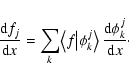
First, let us define the two filters hand g that can be deduced from the MRA. This analysis allows us to determine a function h, which is the impulse response of some $2\pi$-periodic low-pass filter H defined with the scaling function: $H(\omega)=\widehat{\phi}(2\omega)/\widehat{\phi}(\omega)$. On the other hand, one defines function gby $G(\omega)=\widehat{\psi}(2\omega)/\widehat{\phi}(\omega)$, g being the impulse response of the $2\pi$-periodic high-pass filter G. The filters H and G are quadratic mirror filters and are linked by the relation $G(\omega)={\rm e}^{-{\rm i}\omega}\overline{H(\omega+\pi)}$, giving g(n) = (-1)^1-nh(1-n) for the impulse responses. Then, the pyramidal architecture for computing the wavelet representation can be easily written as:

• suppose that f(x_i) belongs to the V₀ ( f(x_i)=f₀(x_i)approximation of the signal at resolution 1) and decompose f(x_i) onto V_-1and W_-1;

• the decomposition onto V_-1 consists in a convolution by the filter $\widetilde h,$ such that $\widetilde h(n) = h(-n)$, and a decimation (i.e. only one out of every two sample is retained); we obtain the N/2-sampled so-called approximation at resolution 1/2equal to
  
  $$f_{-1}(n)=\sum_{n=1}^N \widetilde h(2k-n)f_0(n) \in V_{-1}.$$
  
  

• the decomposition onto W_-1 consists in a convolution by filter $\widetilde g$ (such that $\widetilde g(n)=g(-n)$) and a decimation; we obtain in the same way
  
  $$d_{-1}(n)= \sum_{n=1}^N \widetilde g(2k-n) f_0(n) \in W_{-1};$$
  
  
  this is the detail at resolution 1/2, that is to say the "difference in information'' between f₀(n) and f_-1(n); it also has N/2 samples.

By repeating the same sequence, we obtain the approximation and the detail at resolution 1/2²:

$$f_{-2}(n)= \sum_{n=1}^{N/2} \widetilde h(2k-n) f_{-1}(n) \in V_{-2}$$

and

$$d_{-2}(n)= \sum_{n=1}^{N/2} \widetilde g(2k-n) f_{-1}(n) \in W_{-2} ,$$

and so on.

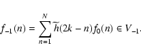
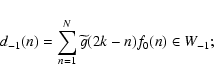
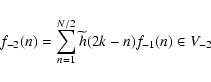
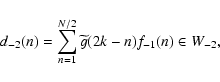
After a number J of iterations to be defined by the problem, we have decomposed f₀ into $d_{-1},\ d_{-2},\ldots,d_J$, and f_J.

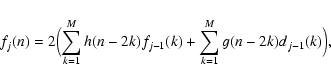
Let us finally mention that reconstruction of f₀(n) from the details and the last approximation is just as easy and has appreciable quality. One has to iterate (starting from j=J):

$$f_j(n)=2\Bigl( \sum_{k=1}^M h(n-2k) f_{j-1}(k) \allowbreak + \sum_{k=1}^M g(n-2k) d_{j-1}(k) \Bigr),$$

f_j-1 and d_j-1 being sampled in M points.

The MRA can be generalised to two dimensions for image-processing applications. We can define a sequence of multi-resolution vector spaces and the approximations of a signal $f(x,y) \in L^2({\rm I\!R}^2)$(Mallat 1989). Since the image under study is bounded, we choose $\phi$with a compact support (i.e. vanishes outside a finite region). In that case, filters h and g have only finitely many coefficients that satisfy the MRA conditions (Daubechies 1992). Functions $\phi$ and $\psi$ become more regular as the number of coefficients n increases (the case of n=1 corresponds to the discontinuous Haar basis). It has been proved (Daubechies 1992) that the regularity of $\phi$ and $\psi$ increases linearly with n. By choosing n=8, we obtain a good compromise between regularity and support width.

References

• Adrian, R. J. 2005, Experiments in Fluids, 39, 159 [NASA ADS] [CrossRef] (In the text)
• Beylkin, G. 1992, SIAM J. Numer. Anal., 6, 1716 [NASA ADS] [CrossRef]
• Bovelet, B., & Wiehr, E. 2001, Solar Phys., 201, 13 [NASA ADS] [CrossRef] (In the text)
• Daubechies, I. 1992, Ten lectures on wavelets (SIAM)
• Mallat, S. 1989, IEEE Trans. on Pat. An. and Mach. Int., 11, 674 [NASA ADS]
• Mallat, S. 1999, A guided tour of signal processing (Academic Press)
• Meyer, Y. 1987, in wavelets, time-frequency methods and phase space, ed. J. M. Combes, A. Grossmann, & P. Tchamitchian (Springer Verlag), 21
• Muller, R., Auffret, H., Roudier, T., et al. 1992, Nature, 356, 322 [NASA ADS] [CrossRef] (In the text)
• November, L. J., & Simon, G. W. 1988, ApJ, 333, 427 [NASA ADS] [CrossRef] (In the text)
• Potts, H. E., Barrett, R. K., & Diver, D. A. 2003, Sol. Phys., 217, 69 [NASA ADS] [CrossRef] (In the text)
• Rieutord, M., Roudier, T., Ludwig, H.-G., Nordlund, Å., & Stein, R. 2001, A&A, 377, L14 [NASA ADS] [CrossRef] [EDP Sciences] (In the text)
• Roudier, T., Rieutord, M., Malherbe, J., & Vigneau, J. 1999, A&A, 349, 301 [NASA ADS]
• Sahiner, B., & Yagle, A. E. 1993, IEEE Trans. on Signal Proc., 41, 3579 (In the text)
• Simon, G. W., Brandt, P. N., November, L., Shine, R., & Strous, L. 1995, in Proc. of 4th SOHO Workshop: Helioseismology (ESA SP-376), 223
• Soille, P. 1999, Morphological Image Analysis (Berlin: Springer)
• Strous, L. 1995, in Proc. of 4th SOHO Workshop: Helioseismology (ESA SP-376), 213 (In the text)
• Tkaczuk, R., Rieutord, M., Meunier, N., & Roudier, T. 2007, A&A, 471, 695 [NASA ADS] [CrossRef] [EDP Sciences] (In the text)
• Vincent, L., & Soille, P. 1991, IEEE Transactions on Pattern Analysis and Machine intelligence, 13, 583 [CrossRef]