A&A 471, 7-15 (2007)
DOI: 10.1051/0004-6361:20077413

Full Boltzmann-kinetical treatment of an ion plasma crossing an MHD shock: parallel and non-parallel cases

M. Siewert - H.-J. Fahr

Argelander Institut für Astronomie der Universität Bonn, Abteilung f. Astrophysik und Extraterrestrische Forschung, Auf dem Huegel 71, 53121 Bonn, Germany

Received 5 March 2007 / Accepted 24 May 2007

Abstract
Aims. We attempt to describe kinetic properties of the solar wind termination shock (and similar MHD shocks in general) using the appropriate form of the kinetic Boltzmann equation, for arbitrary inclinations $\Theta_{Bn}$ between the magnetic field and the shock normal.
Methods. In order to understand the deviations from the perpendicular shock, for which we have already derived an exact solution in an earlier publication, we first prove that our current Boltzmann equation is unable to describe a stationary quasiparallel shock. To ease and open up further research, we derive conditions for the specific form of the relevant Boltzmann equation.
Results. We demonstrate that the simplest Boltzmann equation aiming to describe a parallel MHD shock is in conflict with the predictions from pure MHD. We identify several possible reasons for this, and likewise derive conditions based on the mass flow conservation which must be fulfilled for the shock to be stationary. Assuming that a model for (quasi-)stationary shocks does exist, we are able to explain the unchanged power law index at the passage of the solar wind termination shock observed by the Voyager 1 spacecraft in 2004. We also show that different dissipation mechanisms lead to different transition scales for perpendicular and parallel MHD shocks, and that these differences in the dissipation process also need to be included in the case-competent Boltzmann equation.

Key words: plasmas - shock waves - magnetohydrodynamics (MHD) - solar wind

1 Introduction

Magnetohydrodynamics (MHD) is the most successful theory so far capable of describing astrophysical shocks, such as the solar wind termination shock, planetary bowshocks, or supernova shock waves. The shocks are usually described in the form of jump conditions, which are based on the conservation of certain flows of physical quantities, such as the mass flow, the momentum, and the energy flows (for more recent different model approaches concerning the multifluid properties of the solar wind termination shock see Zank et al. 1993; Chalov & Fahr 1995; Fahr & Scherer 2005; Chalov & Fahr 1994; Zank 1999; Chalov & Fahr 1996). For a magnetized plasma, the jump conditions are usually used in the form given by Serrin (1959), Zel'dovich & Raizer (1966), Landau & Lifshitz (1977) or Diver (2001). However, there are several problems with the MHD treatment of the shock. First and foremost, this approach only works for collision-dominated shocks, guaranteeing an effective equilibrium of the distribution functions. But there are many kind of shocks where this condition is not fulfilled, such as solar wind bowshocks found near astrophysical objects (comets or planets), shocks forming in corotating interaction regions, traveling interplanetary shocks, or the heliospheric termination shock.

Another, less popular problem related to the MHD treatment of astrophysical shocks is the fact that the jump conditions for the lower moments of the distribution function are underdetermined, which means that there remains one variable that cannot be determined by the set of jump conditions alone. Usually, this variable is selected to be the downstream pressure anisotropy, $\lambda=p_\perp/p_\parallel$, since in most physical situations, the dependence of the system on this parameter is very weak (see, e.g. Erkaev et al. 2000). Nevertheless, the MHD description of a shock transition is not complete; in particular the dissipation mechanisms producing entropy are not specified. Even without going into too much detail, it is well known that a full understanding of such processes requires the knowledge of the full upstream and downstream distribution functions, including its dependence upon time and position, which is clearly not provided by a simple set of MHD jump conditions (or, for that part, MHD itself, where the distribution function is reduced to a few low-order velocity moments, while only the knowledge of all these moments is equivalent to a distribution function.

In addition, recently, several spacecraft missions have provided us with directly measured data of the immediate upstream and downstream distribution functions around several astrophysical shocks. The Voyager 1 spacecraft took data on the solar wind termination shock (Stone et al. 2005; Burlaga et al. 2005; Gurnett & Kurth 2005; Decker et al. 2005), observing power law spectra with identical power law indices on both sides of the transition region (Cummings et al. 2006). The Cluster mission consists of four identical spacecrafts able to observe the dynamics of the terrestrial bowshock on a much larger scale (Escoubet et al. 1997); observations from these satellites hint that the shock is highly nonstationary (see e.g. Lobzin et al. 2007).

While numerical simulations are, in principle, able to model such systems with rather high accuracy using shock simulation calculations within hybrid or full particle codes (e.g., see Hada et al. 2003; Scholer et al. 2003), these simulations are, nevertheless, numerical, which makes understanding the physics beyond the results somewhat difficult. In many situations, these simulations, especially in case of quasiparallel shocks, do not show a regular shock shape, but a highly irregular profile. This is, in principle, in good agreement with Cluster observations; however, there are no theoretical, physical explanations for these results yet (Lobzin et al. 2007).

Recently Krasnoselskikh et al. (2002) have investigated the non-stationarity of strong collisionless quasiperpendicular shocks and thereby have compared available theoretical results with full particle numerical simulations. They have proposed an analysis of the shock stationarity based on the theory of nonlinear waves. As it turns out, for those shocks with supercritical Mach numbers the region, where an abrupt increase of the magnetic field occurs, can be treated as a nonlinear whistler wave of large amplitude. They show that beyond some linear whistler Mach number M_A,w no stationary linear wave trains can survive in the shock precursor, i.e. stand still ahead of the field ramp, but are swept into the ramp and pile up there to form a strongly nonlinear whistler wave. This critical Mach number is found by the expression

$$M_{A,w}=\frac{1}{2}\sqrt{\frac{m_{\rm i}}{m_{\rm e}}}\cos\Theta_{B,n}%$$ (1)

and shows that oblique shocks can still appear as stationary even for large Mach numbers of the order of M_A,w $\geq21$. At even larger Mach numbers, however, i.e. beyond the so-called nonlinear whistler Mach number $\breve{M}_{A,w},$ even the nonlinear whistler wave structure cannot be balanced anymore by the effects of dispersion and dissipation. This is the case when the scale of the ramp structure becomes shorter than the dispersion length or the ion inertial length $\lambda_{\rm i}=(c/\omega_{\rm i})\left\vert \cos\Theta_{B,n}\right\vert$. Under these conditions two-fluid MHD approaches are needed in which, depending on the value of $\lambda_{\rm i}$, electron inertia can either be neglected or needs to be taken into account. Above critical Mach numbers of $\breve{M}_{A,w}$ the ramp structure becomes unstable itself, i.e. decays into a time-dependent multi-ramp system. This supercritical Mach number according to Krasnoselskikh et al. (2002) is given by $\breve{M}_{A,w}% =\sqrt{2}M_{A,w}$.

In face of these difficulties, we have recently developed a completely different approach, based on kinetic equations (Fahr & Siewert 2006), aiming to describe the solar wind termination shock, although our results should offer considerably more application opportunities. Especially, our approach should be able to cross the gap between a numerical treatment of many particles in a box, where one is always in danger of overemphasizing numerics over physics, and the MHD treatment, which may be insufficient in face of highly nonstationary processes, as hinted in numerical simulations (Hada et al. 2003; Scholer et al. 2003).

So far, we have successfully applied our model to close the set of anisotropic jump conditions for the purely perpendicular shock, suggesting that our approach leads to physical results. In addition, our approach should prove useful as a test case for numerical codes aiming to simulate the creation and behavior of astrophysical shocks. (Of course, these simulations do likewise present a possibility to test our kinetic approaches.)

While the perpendicular shock leads to a simple and analytic relation between the upstream plasma and the downstream plasma (see Eq. (6)), up to now, for an arbitrary inclination between the magnetic field and the plasma flow, we were unable to arrive at a physical downstream distribution function. In this paper, we greatly expand our previous analysis of the parallel shock, and obtain an improved description of the physics which one has to respect when aiming to understand quasiparallel shocks in astrophysical plasmas.

2 The Boltzmann equation for the shock

2.1 Recent work

In a recent paper (Fahr & Siewert 2006) we have derived the Boltzmann equation for the distribution function $f(w_\parallel,w_\perp,s)$ of a collisionless magnetized plasma crossing an MHD shock, where $w_{\parallel,\perp}$ are the velocity components of the individual plasma particles parallel and perpendicular to the magnetic field. The equation is written in the accelerated reference frame co-moving with the bulk velocity $\vec{U}$, and s is the streamline coordinate in the direction of the shock normal. In the most simple configuration, when only the deceleration of the ions across the shock is considered, the Boltzmann equation takes the form

$$\frac{\rm d}{{\rm d}s} f(w_\parallel,w_\perp,s) = A_\parallel... ... A_\perp \frac{\rm d}{{\rm d}w_\perp} f(w_\parallel,w_\perp,s)$$ (2)

with

  

$$A_\parallel = -\displaystyle \frac{U_n}{U_n + w_\parallel \cos\Th... ...n}\frac{{\rm d}U_n}{{\rm d}s} + w \frac{\rm d}{{\rm d}s} \cos\Theta_{Bn}\right)$$ (3)

$$A_\perp = -\frac{U_n}{U_n + w_\parallel \cos\Theta_{Bn}} \left(\f... ...2B} \frac{{\rm d}B}{{\rm d}s} + w \frac{\rm d}{{\rm d}s} \sin\Theta_{Bn}\right)$$ (4)

where $\Theta_{Bn}$ is the angle between the magnetic field B and the shock normal and U_n is the normal bulk velocity of the plasma. We note that these quantities are usually not constant, but are functions of s in the transition region of the shock. For general cases, this equation needs to be solved numerically, which introduces additional complications in terms of boundary conditions to be imposed on the numerical method. In addition, however, many numerical methods used to solve partial differential equations require the addition of further, "stability''-generating terms, which may be interpreted as the presence of additional terms in the initial equation (see Press 1987-2002, Chap. 19).

An alternate approach is to multiply this equation by parallel and perpendicular velocities, integrate over velocity space, and obtain differential equations for the change of a few selected velocity moments, which corresponds to the pure MHD treatment. However, in this situation, as in common MHD, one is again faced with a hierarchy of momentum equations which need to be closed. In addition, nonlinear terms such as $(U_n + w_\parallel \cos\Theta_{Bn})^{-1}$ introduce terms which may no longer be identified with the usual MHD moments, complicating the situation even further. For these reasons, we now attempt to solve this equation analytically.

 

For a purely perpendicular shock ( $\Theta_{Bn,1,2} = \pi/2$), where the subscripts 1 and 2 denote the upstream and downstream sides of the shock, the Boltzmann equation reduces to

$$\frac{\rm d}{{\rm d}s} f(w_\parallel,w_\perp,s) = -\frac{w_\p... ...m d}s} \frac{\rm d}{{\rm d}w_\perp} f(w_\parallel,w_\perp,s).$$ (5)

In Fahr & Siewert (2006) and Siewert & Fahr (2007), we have demonstrated that practically all MHD properties of the plasma do not depend on the fine structure (i.e. the transition scale) itself. This includes the velocity distribution function,

$$f_2(w_\parallel,w_\perp,s) = f_1 \left(w_\parallel,\frac{w_\perp}{\sqrt{x}} \right),$$ (6)

and the velocity moments,

a_ij,2 = x^(1+i/2) a_ij,1, (7)

which are defined as

$$a_{ij} = \left\langle w_\parallel^i w_\perp^j f(w_\parallel,w... ...nt {\rm d}^3w w_\parallel^i w_\perp^j f(w_\parallel, w_\perp).$$ (8)

These relations have been derived using a separation ansatz (Siewert & Fahr 2007) and are not an approximation, but an exact result. This result allows to describe what happens with a specific upstream distribution function at the crossing of a perpendicular shock. One especially interesting result is that power law spectra, as they have been predicted and observed widely in astrophysics (see e.g. Fisk & Gloeckler 2006; Schlickeiser 2002), are preserved with respect to their power law index when crossing a shock; should a similar result also hold for arbitrary inclinations of the magnetic field, we might have the explanation for the Voyager 1 data (Cummings et al. 2006)

Unfortunately, for the purely parallel shock, we encountered several technical problems (Fahr & Siewert 2006), mainly related to a singularity at $w_\parallel = -U_n$ in Eqs. (3) and (4), which need to be interpreted and treated in a physical way. For a purely parallel shock, the Boltzmann equation reduces to

$$\frac{\rm d}{{\rm d}s} f(w_\parallel,w_\perp,s) = -\frac{U_n... ...}s} \frac{\rm d}{{\rm d}w_\parallel} f(w_\parallel,w_\perp,s).$$ (9)

This expression is not solvable using a separation ansatz, since the term proportional to $\frac{w_\parallel}{U_n + w_\parallel}$, which appears in Eq. (4), excludes such an approach.

2.2 The almost perpendicular shock

Aiming to understand the parallel shock better, we now estimate whether this configuration is the exception where our equation fails, or if, perhaps, the perpendicular shock is the only configuration where our equation works. In order to do this, we investigate the quasi-perpendicular shock ( $\Theta_{Bn}= \pi/2 - \Delta \alpha$), and develop the Boltzmann equation around $\pi/2$, leading to

$$\left. \frac{\rm d}{{\rm d}s} f \right\vert _{\pi/2 - \Delta ... ...ft(\frac{{\rm d}f}{{\rm d}s} \right) \right\vert _{\pi/2}\cdot$$ (10)

In this equation the first term on the right hand side (RHS) represents the regular term in the perpendicular equation (Eq. (5)), which adequately describes the purely perpendicular shock (Siewert & Fahr 2007), while the other term is the first-order (linear) correction for an angle $\alpha = \pi/2 - \Delta\alpha$.

The second term on the RHS of Eq. (10) may be evaluated starting from the general form of the Boltzmann equation (Eq. (2)), leading to

 

$$\displaystyle\frac{\rm d}{{\rm d}\alpha} \left( \frac{{\rm d}f}{{... ...} + A_\perp \displaystyle\frac{{\rm d}^2f}{{\rm d}\alpha \ {\rm d}w_\perp}\cdot$$ (11)

The partial derivatives with respect to $\alpha$ may be evaluated to

$$\displaystyle\frac{{\rm d}A_\parallel}{{\rm d}\alpha}-\displaysty... ...alpha \frac{{\rm d}U_n}{{\rm d}s} + w \frac{\rm d}{{\rm d}s} \sin\alpha \right)$$ (12)

$$\displaystyle\frac{{\rm d}A_\perp}{{\rm d}\alpha} = -\displaystyl... ...+ w_\parallel \cos\alpha} w \displaystyle\frac{\rm d}{{\rm d}s} \cos\alpha\cdot$$ (13)

Taking $\alpha(s) \equiv \pi/2$, most of the above terms vanish, and we obtain

$$\left. \displaystyle\frac{{\rm d}A_\parallel}{{\rm d}\alpha} \right\vert _{\alpha = \pi/2} =- \displaystyle\frac{{\rm d}U_n}{{\rm d}s}$$ (14)

$$\left. \displaystyle\frac{{\rm d}A_\perp}{{\rm d}\alpha} \right\v... ...\frac{w_\perp}{2} \frac{\rm d}{{\rm d}s} \ln B \frac{{\rm d}U_n}{{\rm d}s}\cdot$$ (15)

Since, per definition, f does not depend upon $\alpha$, but only on s, we may rewrite the second order-derivatives as

$$\frac{{\rm d}^2f}{{\rm d}\alpha \ {\rm d}w_i} = \frac{{\rm d}... ...m d}s \ {\rm d}w_i} \cdot \frac{{\rm d}s}{{\rm d}\alpha}\cdot$$ (16)

Since we only need to evaluate this expression for $\alpha = \pi/2$, where, in this special configuration, there is no functional connection between the two quantities s and $\alpha$, we automatically see that the second-order derivatives identically vanish. In the more general case, the expression d$\alpha/$ds is given by

$$\frac{{\rm d}\alpha}{{\rm d}s} = \frac{\rm d}{{\rm d}s} \hbox... ... \frac{B_n B_{n1}}{B_t^2 B_{t1}} \frac{{\rm d}U_n}{{\rm d}s},$$ (17)

which is zero for the perfectly perpendicular shock. We would like to emphasize that this is only one of several possible representations of d$\alpha$/ds; especially for $\alpha=0$, there is no divergence.

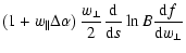
Taking these results together, we may write Eq. (10) in the form

 

$$\frac{\rm d}{{\rm d}s} f \simeq \Delta\alpha \frac{{\rm d}U_n}{{\rm d}s} \frac{{\rm d}f}{{\rm d}w_\parallel}$$ -

$$\left( 1 + w_\parallel \Delta\alpha \right) \frac{w_\perp}{2} \frac{\rm d}{{\rm d}s} \ln B \frac{{\rm d}f}{{\rm d}w_\perp}$$ -

$$A_{\parallel,\Delta\alpha} \frac{{\rm d}f}{{\rm d}w_\parallel} + A_{\perp,\Delta\alpha} \frac{{\rm d}f}{{\rm d}w_\perp},$$ = (18)

where

 

$$A_{\parallel,\Delta\alpha} = - \Delta\alpha \frac{{\rm d}U_n}{{\rm d}s}$$ (19)

$$A_{\perp,\Delta\alpha} = - \left(1 + w_\parallel \Delta\alpha \right) \frac{w_\perp}{2} \frac{\rm d}{{\rm d}s} \ln B.$$ (20)

2.3 The Boltzmann equation in the rest frame of the parallel shock

In this analysis, we now also consider the Boltzmann equation in the non-accelerated rest frame of the standing transition region, which we derive now. This approach may be useful to estimate which terms in Eq. (2) are more "problematic'' than others. We would also like to note that, as we are working in the non-relativistic limit, the Boltzmann equation derived in the co-moving accelerated rest frame of the plasma stream should be qualitatively identical with the equation one would derive in the inertial rest frame of the shock transition region. In fact, most of the terms in the Boltzmann equation may be derived exactly in the same way as in Fahr & Siewert (2006), which means we only need to emphasize the changes.

In a more general form, the Boltzmann equation is written as

$$(\vec{w} \cdot \nabla_x)f(w,x) + (\vec{F} \cdot \nabla_w)f(w,x) = 0,$$ (21)

where $(F\cdot \nabla_w)$ is the force term, and $(w \cdot \nabla_x)$ is the drift term, describing changes in velocity and configuration space, respectively. Following the transformation into an inertial reference frame, we must remove the convective term and the pseudo forces, and replace these terms with the (now physical, i.e. Newtonian) force responsible for the deceleration. Usually, it is assumed that a local electric potential wall develops as consequence of the electric charge concentrations on both sides of the transition region, which in turn create electric fields and decelerates the upstream ions. For this reason, we now derive the MHD prediction of this additional, Newtonian force term in the case of the purely parallel shock. Assuming that the shock transition region is only a function of the streamline coordinate s, we may write the force term in the form

$$F_s \frac{\rm d}{{\rm d}w_\parallel} f = -\frac{e}{m} E(s) \frac{\rm d}{{\rm d}w_\parallel} f.$$ (22)

For simplicity, we will omit the f in the following steps, reducing the equation to an operator. In addition, we define the charge-to-mass ratio $e/m \equiv \mu$. Finally, we restrict ourselves to the parallel shock.

The electric field E(s) may be derived from the MHD equation of ion motion, which is given for a one-dimensional system in the form

$$\rho U \frac{{\rm d}U}{{\rm d}s} = - \frac{{\rm d}P}{{\rm d}s} + \mu \rho E,$$ (23)

where P is the local pressure. Solving this equation for the electric fields E then yields

$$E = (\mu \rho)^{-1} \left( \rho U \frac{{\rm d}U}{{\rm d}s} + \frac{{\rm d}P}{{\rm d}s} \right).$$ (24)

Using the polytropic relation $C = P/\rho^\gamma$ (with the polytropic index $\gamma$), we obtain

$$E = (\mu \rho)^{-1} \left( \rho U \frac{{\rm d}U}{{\rm d}s} +... ...mma \rho^{\gamma - 2} \frac{{\rm d}\rho}{{\rm d}s}\right)\cdot$$ (25)

Introducing the constant mass flow $F = \rho U$, we may furthermore write

$$E = (\mu \rho)^{-1} U \frac{{\rm d}U}{{\rm d}s} \left( 1 - \f... ...ho_1 U_1^2} \left( \frac{U_{1}}{U} \right)^{\gamma+1}\right),$$ (26)

and finally, using $c_{s1}^2 = \gamma P_1/\rho_1$ and M₁ = U₁/c_s1,

$$E = (\mu \rho)^{-1} U \frac{{\rm d}U}{{\rm d}s} \left( 1 - \frac{1}{M_1^2} \left( \frac{U_{1}}{U} \right)^{\gamma+1} \right).$$ (27)

Inserting this into Eq. (22), we obtain the following force term to our Boltzmann equation:

$$U \frac{{\rm d}U}{{\rm d}s} \left( 1 - \frac{1}{M_1^2} \left... ...ght)^{\gamma+1} \right) \frac{\rm d}{{\rm d}w_\parallel} \cdot$$ (28)

Obviously, the first term in this equation exactly yields the pseudo force term responsible for the bulk deceleration of the system. If we want that this equation is identical to the Boltzmann equation derived in the accelerated reference frame, we obtain the condition

$$U \frac{{\rm d}U}{{\rm d}s} \frac{1}{M_1^2} \left( \frac{U_{1... ...d}{{\rm d}w_\parallel} \stackrel{!}{=} \frac{\rm d}{{\rm d}t},$$ (29)

i.e. we (should) have derived an expression for the convective change of the distribution function in the solar wind rest frame. However, on a closer look, this analogy does not hold perfectly, as the distribution function is different in both reference frames, too.

   
3 Solving the Boltzmann equation

To solve the Boltzmann equation for an arbitrary angle $\Theta_{Bn}$, we use the representation

$$f(w_\parallel,w_\perp,s) = f_1(\bar{w}_\parallel(w,s), \bar{w}_\perp(w,s)),$$ (30)

which means that on the downstream side of the shock, the ions are expected to be distributed, essentially, conformally invariant, however with new, s-dependent variables, where the modified variables $\bar{w}_\parallel$ and $\bar{w}_\perp$describe the distortion. Taking the derivative with respect to s, and assuming that there is no explicit time-dependence, we obtain

$$\frac{{\rm d}f}{{\rm d}s} = \frac{{\rm d}f}{{\rm d} \bar{w}_\... ... d} \bar{w}_\perp} \frac{{\rm d} \bar{w}_\perp}{{\rm d}s}\cdot$$ (31)

Using the method of comparing coefficients, and a Boltzmann equation of the form given in Eq. (2), we then obtain the relations

  

$$\frac{\rm d}{{\rm d}s} \bar{w}_\parallel = A_\parallel(\bar{w},s)$$ (32)

$$\frac{\rm d}{{\rm d}s} \bar{w}_\perp = A_\perp(\bar{w},s).$$ (33)

These expressions represent two differential equations which, applying the parameters for our Boltzmann equation (Eqs. (3) and (4)), are of the first order and coupled (because of the terms proportional to $w = \sqrt{w_\parallel^2+w_\perp^2}$). Usually, solving these equations for $\bar{w}_\parallel$ and $\bar{w}_\perp$ requires a numerical procedure, using the initial conditions

$$\bar{w}_\parallel(s_1) = w_\parallel \bar{w}_\perp(s_1) = w_\perp.$$ (34)

Thus we have reduced the initial partial differential equation (PDE) to two ordinary differential equations (2ODE), which is an improvement from a numerical point of view.

3.1 The perpendicular shock revisited

To verify that the ansatz presented in Eq. (30) does not contradict earlier results, we first demonstrate that the exact solution for the perpendicular shock (Siewert & Fahr 2007),

$$f_2(w_\parallel,w_\perp) = f_1 \left(w_\parallel, \frac{w_\perp}{\sqrt{x}} \right),$$ (35)

is reproduced, where x is the MHD compression ratio. The Boltzmann equation for the purely perpendicular shock is

$$\frac{{\rm d}f}{{\rm d}s} = - \frac{w_\perp}{2} \frac{\rm d}{{\rm d}s} (\ln B) \frac{{\rm d}f}{{\rm d}w_\perp}\cdot$$ (36)

Solving the differential Eqs. (32) and (33) trivially leads to $\bar{w}_\parallel = w_\parallel$ and to

$$\bar{w}_\perp = w_\perp \exp \left( - \frac{1}{2} \int_{s_1}^s \ln B(s) \ {\rm d}s \right) = \frac{w_\perp}{x(s)}\cdot$$ (37)

Thus we can already conclude that this result supports the representation (30), where the Boltzmann equation is reduced to two ODEs.

   
3.2 The parallel shock

Next, we investigate the purely parallel shock ( $\Theta_{Bn}= 0$), where the Boltzmann equation reduces to Eq. (9), which automatically leads to

$$\bar{w}_\perp \equiv w_\perp,$$ (38)

while $\bar{w}_\parallel$ is the solution of the differential equation

$$\frac{\rm d}{{\rm d}s} \bar{w}_\parallel = -\frac{U_n}{U_n + \bar{w}_\parallel} \frac{{\rm d}U_n}{{\rm d}s}\cdot$$ (39)

This is a nonlinear (and therefore nontrivial) problem, although it is possible to verify numerically that this relation automatically leads to an additional deceleration of the system. However, since numerical methods are, in principle, prone to errors, we now present an analytical proof for this.

Since our Boltzmann equation has been explicitly derived in the co-moving accelerated MHD reference frame, the parallel velocity moment,

$$U_{\parallel,2} = \langle w_\parallel \rangle _2 = \int {\rm d}^3w \ w_\parallel \ f_2(w),$$ (40)

should always be zero. This condition may be verified by taking the differential Eq. (9), multiplying it with $w_\parallel$ and integrating over d³w, leading to

$$\int {\rm d}^3w \ w_\parallel \frac{\rm d}{{\rm d}s} f \frac{\rm d}{{\rm d}s} U_\parallel$$ =

$$-\int {\rm d}^3w \frac{U_n w_\parallel}{U_n + w_\parallel} \frac{{\rm d}U_n}{{\rm d}s} \frac{\rm d}{{\rm d}w_\parallel} f.$$ = (41)

Clearly, this is a differential equation for the change of the parallel velocity moment across the shock. Because of our choice of the reference frame, it should be equal to zero for all s. Applying the substitution

$$U_n(s) + w_\parallel = x,$$ (42)

we obtain

$$0 \stackrel{!}{=} -2\pi U_n \frac{{\rm d}U_n}{{\rm d}s} \int_... ...ty {\rm d}x \ \frac{x - U_n}{x} \frac{{\rm d}f}{{\rm d}x}\cdot$$ (43)

Since we are only considering nontrivial configurations, we get $U_n(s) \neq 0$, and since we are attempting to model a shock, where a deceleration does exist, we obtain dU_n/d$s \neq 0$ as well, and our condition reduces to

 

$$\stackrel{!}{=} -\int_0^\infty {\rm d}w_\perp \int_{-\infty}^\infty {\rm d}x \frac{x - U_n}{x} \frac{{\rm d}f}{{\rm d}x}$$                          0

$$-\int_0^\infty {\rm d}w_\perp \int_{-\infty}^\infty {\rm d}x \left( 1 - \frac{U_n}{x} \right) \frac{{\rm d}f}{{\rm d}x}$$ =

$$U_n \int_0^\infty {\rm d}w_\perp \int_{-\infty}^\infty {\rm d}x \frac{1}{x} \frac{{\rm d}f}{{\rm d}x}\cdot$$ = (44)

Assuming that a physical, non-trivial distribution function f exists, we partially integrate it, leading to

 

$$\stackrel{!}{=} U_n \int_0^\infty {\rm d}w_\perp \left( \left[ \frac{f(x)}{x} \right]_{-\infty}^\infty + \int_{-\infty}^\infty f(x) \frac{1}{x^2} {\rm d}x \right)$$                          0

$$\int_0^\infty {\rm d}w_\perp \int_{-\infty}^\infty f(x) \frac{1}{x^2} {\rm d}x.$$ = (45)

For a physical distribution function (i.e. $f(w) \geq 0$), the integrand is always larger than zero, which means that, as long as $U_n \neq 0$, the only way to obtain a vanishing kinetic parallel velocity in the co-moving accelerated MHD reference frame is to set $f(x) \equiv 0$, i.e. working in a vacuum. This result clearly proves that our Boltzmann equation is inherently unable to describe the parallel MHD shock, as there is always a finite difference between the MHD and the kinetic co-moving reference frames.

3.3 The almost perpendicular shock

Finally, we consider the almost perpendicular shock, i.e. just an infinitesimal step from the situation where our approach works. In this case, it automatically follows from Eqs. (19) and (32) that this Boltzmann coefficient describes a systematic deceleration of the upstream velocity distribution function away from the co-moving reference frame, on top of the implicit MHD deceleration at the shock.

To improve our analysis, we now repeat the arguments presented in Sect. 3.2, taking the parallel Boltzmann equation in the rest frame of the shock,

$$w_\parallel \frac{\partial}{\partial s} f = -U_n \frac{{\rm d}U_n}{{\rm d}s} \frac{\partial}{\partial w_\parallel} f,$$ (46)

and integrating it over d³w, leading to

$$\frac{\partial}{\partial s} U_\parallel = - U_n \frac{{\rm d}... ...s} \int {\rm d}^3w \ \frac{\partial}{\partial w_\parallel} f.$$ (47)

For a physical distribution function, the integral is proportional to

$$\int_{-\infty}^\infty {\rm d}w_\parallel \frac{{\rm d}f}{{\rm d}w_\parallel} \equiv 0,$$ (48)

suggesting that an upstream parallel plasma should not be affected by this equation at all, while a deceleration should occur in this reference frame. Taken together with the earlier result for the accelerated reference frame, both results hint that the only solution to a parallel shock may be the trivial $x_{\rm MHD}=1$ situation, i.e. the distribution function is not affected by the shock at all. From these results we automatically see that the systematic deceleration of the upstream plasma flow may not be attributed to the electric field gradient of the single-ion plasma in the transition region, leading us to the conclusion that a simple kinetic description is inherently unable to describe an MHD shock in a single-fluid plasma.

4 Necessary properties for physical downstream distribution functions

4.1 The MHD mass flow

Is it at all possible, for a solution of an equation of the form (2), to find a combination of functions $A_\parallel$ and $A_\perp$ which is not in conflict with MHD? We now attempt to answer this question by going deeper into the underlying mathematical structures.

We begin with the most simple MHD jump condition, the mass flow conservation,

$$\rho_1 U_{n1} = \rho_2 U_{n2},$$ (49)

which must always be valid for a source-free fluid system. (If this were not the case, particles would be stopped inside or reflected from the transition region, leading to two-stream instabilities and accumulation of local space charges, requiring additional, carefully balanced terms both on the MHD and the kinetic sides of our problem.) From this condition, it follows that the kinetically devised MHD moments, which are given by Eq. (8), must fulfill the relations

  

$$\rho_2 = x \rho_1$$ (50)

$$U_{\parallel,2} = \langle w_\parallel \rangle _2 = 0,$$ (51)

where the second relation must hold only in the accelerated co-moving reference frame.

Making the ansatz given by Eq. (30), we may write Eq. (50) in integral form,

$$\int {\rm d}^3w \ f_1(\bar{w}_\parallel(w), \bar{w}_\perp(w)) = x \int {\rm d}^3w \ f_1(w_\parallel, w_\perp).$$ (52)

Transforming the LHS of this equation into the new coordinates $\bar{w}(w)$ leads to

$$\int {\rm d}^3w \ f_1(\bar{w}_\parallel(w), \bar{w}_\perp(w))... ... {\rm d}^3\bar{w} \ D \ f_1(\bar{w}_\parallel, \bar{w}_\perp),$$ (53)

where D is the Jacobi determinant associated with the variable transformation.

4.2 Transformation equations for the variables

We now need to estimate which coordinate transformations $w(\bar{w})$are compatible with these relations. Considering that only the upstream parallel velocity moment, $\langle w_\parallel \rangle_1$, identically vanishes on account of the initial assumptions, we require a linear relation between the parallel components,

$$w_\parallel = C_\parallel \bar{w}_\parallel.$$ (54)

If there were any nonlinear terms involved in this relation, the downstream velocity moment would be nonzero in any reference frame because of an admixture of higher-order moments. Similarly, there must be no perpendicular velocity contributions to this relation, which would otherwise lead to an admixture as well. Applying the "natural'' coordinates for this problem, i.e. cylinder coordinates, averaging over the azimuthal angle, and applying Eq. (54), the Jacobi determinant is given by

$$D = \frac{{\rm d}w_\parallel}{{\rm d}\bar{w}_\parallel} \fra... ...perp}{{\rm d}\bar{w}_\perp} \frac{w_\perp}{\bar{w}_\perp}\cdot$$ (55)

This allows us, by applying Eq. (55) to Eq. (52) and Eq. (53), to obtain the relation

$$C_\parallel \frac{{\rm d}w_\perp}{{\rm d}\bar{w}_\perp} \frac{w_\perp}{\bar{w}_\perp} = x.$$ (56)

This is an exact differential equation, which is trivially solved by

 

$$w_\perp = \sqrt{ \frac{x}{C_\parallel} } \bar{w}_\perp = C_\perp \bar{w}_\perp \quad C_\perp = \sqrt{ \frac{x}{C_\parallel} },$$ (57)

demonstrating that the perpendicular coordinates must be connected by a linear relation as well.

This result already allows us to write the most general, particle number conserving downstream ion distribution function as

$$f_2(w_\parallel,w_\perp) = f_1\left( \frac{w_\parallel}{C_\parallel}, \frac{w_\perp}{C_\perp} \right),$$ (58)

where the coefficients $C_\parallel$ and $C_\perp$ must not depend upon w. In addition, the condition

$$C_\parallel \cdot C_\perp^2 = x$$ (59)

must also be fulfilled. This result is in agreement with the perpendicular solution, where $C_\parallel = 1$ and $C_\perp = \sqrt{x}$.

4.3 The functions $A_\parallel$ and $A_\perp$ for our Boltzmann equation

Using the formalism developed in the previous sections, we may now explain why our Boltzmann equations seemingly conflicts with basic MHD. Inserting Eq. (58) into Eq. (2), we obtain

$$\frac{{\rm d}f}{{\rm d}s} \frac{{\rm d}f}{{\rm d}\bar{w}_\parallel} \frac{{\rm d}\bar{w}_\p... ...} + \frac{{\rm d}f}{{\rm d}\bar{w}_\perp} \frac{{\rm d}\bar{w}_\perp}{{\rm d}s}$$ =

$$A_\parallel(w) \frac{{\rm d}f}{{\rm d}w_\parallel} + A_\perp(w) \frac{{\rm d}f}{{\rm d}w_\perp}$$ =

$$A_\parallel(w) \frac{{\rm d}\bar{w}_\parallel}{{\rm d}w_\parallel... ...rac{{\rm d}\bar{w}_\perp}{{\rm d}w_\perp} \frac{{\rm d}f}{{\rm d}\bar{w}_\perp}$$ =

$$\frac{A_\parallel(w)}{C_\parallel} \frac{{\rm d}f}{{\rm d}\bar{w}... ...rallel} + \frac{A_\perp(w)}{C_\perp} \frac{{\rm d}f}{{\rm d}\bar{w}_\perp}\cdot$$ = (60)

Then, by comparing coefficients, we obtain

$$A_\parallel(\bar{w}) \ C_\parallel^{-1} =-\bar{w}_\parallel \displaystyle\frac{ \frac{{\rm d}C_\parallel}{{\rm d}s} }{C_\parallel^2}$$ (61)

$$A_\perp(\bar{w}) \ C_\perp^{-1} = -\bar{w}_\perp \displaystyle\frac{ \frac{{\rm d}C_\perp}{{\rm d}s} }{C_\perp^2}\cdot$$ (62)

These two differential equations for $C_\parallel$and $C_\perp$ may be brought into the standard form

  

$$\frac{\rm d}{{\rm d}s} C_\parallel = -\displaystyle\frac{A_\parallel(w)}{w_\parallel} \cdot C_\parallel = -a_\parallel C_\parallel$$ (63)

$$\displaystyle\frac{\rm d}{{\rm d}s} C_\perp = -\displaystyle\frac{A_\perp(w)}{w_\perp} \cdot C_\perp = -a_\perp C_\perp,$$ (64)

where a_i=A_i/w_i must not depend upon w. If this were not the case, then the resulting C_iwould posses a similar dependence, which in turn would break the mass flow conservation. These equations are formally solved by

$$C_{\parallel,\perp}(s) = \exp \int_{s_1}^s -a_{\parallel,\perp}(s) {\rm d}s,$$ (65)

and Eq. (59) may be written as

$$\ln x(s) = -\int_{s_1}^s (a_\parallel(s) + 2 a_\perp(s)) {\rm d}s,$$ (66)

which allows us to test any pair of Boltzmann coefficients A_i using a simple integration.

Since $a_\parallel$ and $a_\perp$ must not depend on $w_{\parallel,\perp}$, we automatically see that our Boltzmann coefficients given by Eqs. (54) and (57) are only able to describe a simple (i.e. not explicitly time-dependent, not turbulent, etc.) MHD shock for $\Theta_{Bn}\equiv \pi/2$, when the derived coefficients a_i do not depend upon w. For all other magnetic field orientations, the singular factor clearly rules out the required w-dependence.

5 Applications of our formalism

5.1 Relations between the upstream and downstream moments

Using the requirements derived in Sect. 3 for a stationary MHD shock, we may now derive relations between the upstream and downstrem MHD moments; repeating the calculations done by Siewert & Fahr (2007), we obtain

$$a_{ij,2} = C_\parallel^{i+1} C_\perp^{j+2} a_{ij,1},$$ (67)

and, for the downstream pressure anisotropy,

$$\lambda_2 = \frac{p_{\perp,2}}{p_{\parallel,2}} = \frac{C_\perp^2}{C_\parallel^2} \lambda_1\cdot$$ (68)

Using Eq. (59), this expression may be rewritten as

$$\lambda_2 = \frac{x}{C_\parallel^3} \lambda_1 = \frac{C_\perp^6}{x^2} \lambda_1\cdot$$ (69)

According to Erkaev et al. (2000), the jump conditions of the system may be expressed as the solution of two nonlinear polynomial equations for the three unknown variables $\epsilon$, x, and $\lambda_2$, where usually $\lambda_2$ is taken as the undetermined parameter. Now, however, using the additional Eq. (69), it is possible to close the system of jump conditions, as long as the underlying kinetic equation fulfills Eq. (59). This result also proves that, at least in principle, it is possible to arrive at a kinetic description of a stationary MHD shock with arbitrary inclination. Finally, assuming that such a description does exist, it is then trivial to close the MHD jump conditions at a stationary boundary layer; instead, the nontrivial problem is finding the correct kinetic description.

5.2 Power law spectra passing an arbitrarily oriented shock

Next, we would like to point out an interesting fact. Taking Eq. (58), and applying this to a power law distribution function,

$$f_{k,1} \propto w^k \propto w_\perp^k,$$ (70)

we may write for the downstream site

$$f_{k,2} \propto C_\perp^{-k} w_\perp^k,$$ (71)

using precisely the same power k as on the upstream side, as the coefficients C_i do not depend upon w. This result explains the observations made by Voyager 1, where it was, surprisingly, found that the observed solar wind power law index did not change during the event interpreted as the passage over the solar wind termination shock (Cummings et al. 2006). It also gives the theoretical explanation of a result derived by Fisk & Gloeckler (2006), however not based on the assumption of pitch angle isotropic distribution functions.

6 Outlook

6.1 The physics behind the singular factor

In the last sections, we have demonstrated that two simple physical principles, stationarity and mass flow conservation, strongly restrict the Boltzmann coefficients in Eq. (2). We now attempt to understand what kind of physical processes might be compatible with these conditions. In order to do this, we first note that, during the initial derivation of our Boltzmann equation (Fahr & Siewert 2006), we obtained an equation of the form

$$B_t \frac{\partial}{\partial t} f + B_s \frac{\partial}{\part... ...w_\parallel} f + B_\perp \frac{\partial}{\partial w_\perp} f,$$ (72)

where the coefficients B_i are simple, non-singular functions of w and s. Then, using the implicit stationarity, the substitution $\frac{\partial}{\partial t} \rightarrow U_n \frac{\partial}{\partial s}$ was made, followed by a division so that this equation reduced to

$$(U_n B_t + B_s) \frac{\partial}{\partial s} f = B_\parallel ... ...w_\parallel} f + B_\perp \frac{\partial}{\partial w_\perp} f,$$ (73)

where the left handed side (LHS) is equivalent to $(U_n + w_\parallel \cos\Theta_{Bn})$, which is then divided out, giving rise to the global singularity in our A_i.

Obviously, we need to understand the physical meaning behind the LHS. Considering that U_n is the normal bulk velocity of the plasma flow, it is straightforward to interpret the entire term as a differential bulk velocity, i.e. the entire "slice'' of individual particles moving at identical $w_\parallel$ (and arbitrary $w_\perp$) is crossing the shock with a differential velocity of

$$U_n' = U_n + w_\parallel \cos\Theta_{Bn}.$$ (74)

This leads to many differential streams, which in turn leads to many two-stream instabilities, a situation which, to our knowledge, has not been considered theoretically yet. However, this result also hints that, in principle, additional nonlinear processes, such as turbulence and wave-particle interactions, must necessarily appear in a kinetic shock theory.

6.2 The problem of charge neutrality

Furthermore, this analysis points towards another problem, namely the question of charge-neutrality. In MHD, this assumption is usually a requirement, although in many situations, electrons are left out of the analysis because of their small rest masses. This hints that the remedy for that situation must be to include electrons as a separate dynamical population. This is because only in case of the perpendicular MHD shock the system of the plasma bulk velocity is a preferred system, since here the perpendicular magnetic field controlling both the bulk motion of the ions and the electrons is just convected with this bulk velocity system. This causes bulk velocities of ions to be identical with that of electrons, which is no longer the case for non-perpendicular shocks. In the latter case, electrons react completely differently compared to ions to the electric fields inside the transition region. While these fields do decelerate the ions, leading to a very similar term in the Boltzmann equation than the pseudo forces appearing in the co-moving accelerated reference frame, electrons will be accelerated instead; considering the much smaller electron mass compared to the heavier ions, this acceleration should be much larger than the proton deceleration, perhaps even leading into the relativistic regime. This, however, enforces the need to also consider an independent Boltzmann equation for the electrons and, in addition, to couple the two Boltzmann equations for ions and electrons, by addition of adequate friction force terms.

Some general control on this two-population system for the parallel shock (z-direction parallel to $\vec{B}$) is given by standard electrodynamic requirements for this shock. From Maxwells equation $\hbox{rot}\vec{B}=4\pi\vec{j}$, we may conclude for the 1-dimensional shock that

$$\left[ \hbox{rot}\vec{B} \right]_{x} =-\frac{{\rm d}B_{y}}{{\rm d}z}=0$$

$$\left[ \hbox{rot}\vec{B} \right]_{y} =-\frac{{\rm d}B_{x}}{{\rm d}z}=0$$

$$\left[ \hbox{rot}\vec{B} \right]_{z} =4\pi j_{z} \stackrel{!}{=} 0,$$ (75)

which means that the electric current in the transition region always has to vanish, i.e.

j_z=e(n_eU_e-n_pU_p)=0, (76)

and that the electric space charge density $\eta$ is given by

$$\eta=e(n_{p}-n_{e})=en_{p}(1-U_{p}/U_{e}).$$ (77)

6.3 The thickness of the transition region

So far, we have made no specific assumptions on the fine structure of the shock transition region, partially on account of the fact that we have never truly required such assumptions yet. However, the nonstationarity of the shock clearly suggests that this simplification is no longer valid, and that we need to allow for an explicitly extended shock. In this section, as a preparation for further work, we present estimations on how thick the shock might be in the perpendicular and parallel situations.

Roughly spoken the extent of the collision-less shock transition is defined by the length needed in a shock-generated gradient structure to create enough entropy, and dissipate enough kinetic energy of the upstream flow into thermal energy of the downstream flow. The rate of entropy generation, however, strongly depends on the available mechanisms which can effectively work for such dissipations, with the available mechanisms in turn depending on the distribution function of the plasma.

Lee et al. (1986) have considered single ion trajectories through a planar MHD structure in a test particle approach, by parameterizing the planar perpendicular MHD shock by a shock scale $\lambda$ measured in natural ion length units $x_{0}=U_{1}/\Omega_{\rm i}$ (where U₁ is the upstream plasma bulk velocity, and $\Omega_{\rm i}=eB_{t1}/m_{\rm i}c$ is the ion gyrofrequency related to the upstream tangential field component B_t1). They have found that, for a strong shock (i.e. $B_{t2}/B_{t1}\simeq4$), the gyrophase average of the downstream gyrational ion energy first increases with increase of $\lambda$ up to a maximum value $\left\langle E_{g2}\right\rangle \simeq0.35\cdot (m_{\rm i}U_{1}^{2}/2)$ at $\lambda_{\max}=0.25$ and then decreases at further increase of $\lambda$. This downstream gyrational energy $\left\langle E_{g2}\right\rangle$, however, is in a low-entropic form and by no means fulfills the dissipation requirements of Rankine-Hugoniot relations with a conversion rate $\left\langle E_{g2}\right\rangle /(m_{\rm i}U_{1}^{2}/2)=0.75$ of upstream kinetic into downstream thermal energy. Nevertheless from their study it becomes evident that the parameter $\lambda$ can be optimized such that the resulting dissipation attains a maximum. For very small values of $\lambda$, pure ion overshoot will happen, while for large $\lambda$, pure conservation of the magnetic ion moment will occur. Maximum dissipation, however, appears to be in between these two extreme cases. This intermediate case is perhaps realized when an unstationary shock structure eventually becomes stationary just when meeting the right steepness conditions. Though not based on a rigorous theoretical treatment, one may nevertheless draw the qualitative conclusion from it, that the strong perpendicular MHD shock may have a transition scale of $\lambda_{\perp}\simeq0.25\cdot(U_{1}/\Omega_{\rm i})$.

In contrast to the above, a corresponding scale estimate $\lambda_{\parallel}$for the parallel shock has to be elaborated on completely different physical grounds. In this particular case, where B_n1=B_n2 is valid, no dissipation can be achieved by conversion into gyrational energy modes. The only way to realize dissipation is through dynamical coupling between ions and overshooting electrons either by electrostatic or by Whistler wave turbulences which culminates in the requirement (see Quest 1986) that the upstream electron resistive diffusion length $D_{\rm diff}$ be of the order of the ion inertial length $D_{\rm i}\simeq c/\omega_{p,{\rm i}}$ (where $\omega_{p,{\rm i}}=\sqrt{4\pi ne^{2}/m_{\rm i}}$ is the ion plasma frequency). This criterion has been proven to be fairly correctly fulfilled based on corresponding investigations of data obtained with ISEE at several Earth bowshock crossings (Scudder et al. 1986). More recently it has been shown in measurements of the Cluster satellites (Lobzin et al. 2007) that the required anomalous electron resistivity most probably in case of the Earth`s bowshock is enforced by large amplitude Whistler waves which are driven unstable towards some saturation level in the bowshock transition region. These authors are also able to demonstrate that the bowshock structure is unstationary, as long as Whistler wave turbulence amplitudes stay low, and only becomes stationary, if the turbulence amplitudes have reached a supercritical level.

We thus can estimate the transition scale $\lambda_{\parallel}$ of the parallel MHD shock looking for the dimension over which overshooting electrons can couple their kinetic energy via Whistler waves to the shocked ions. Whistler waves in the electron frame have frequencies $\omega$ which in the ion bulk frame are seen with a frequency $\acute{\omega}$ with the following relation valid

$$\acute{\omega}=\omega-k\Delta U$$ (78)

where k is the wave vector of the Whistler wave and $\Delta U$ is the difference in the bulk velocities of protons and electrons. The latter can easily be estimated by the expression

$$\Delta U\simeq U_{{\rm i}2}-U_{e2}\simeq-\sqrt{\frac{m_{\rm i}}{m_{\rm e}}}U_{1}.$$ (79)

Only the left-handed Whistler wave can be absorbed by ions when the Whistler wave frequency is seen in the ion frame as ion cyclotron frequency $\Omega_{\rm i}$, thus requiring as resonance condition a Whistler frequency of

$$\omega_{{\rm i},r}=\Omega_{\rm i}-k_{\rm i}\sqrt{\frac{m_{\rm i}}{m_{\rm e}}}U_{1}%$$ (80)

which can be expressed as a pure function of frequency when using the Whistler wave dispersion relation $k=k(\omega)$ and thus yields

$$\omega_{{\rm i},r}=\frac{\Omega_{\rm i}}{1+\sqrt{\frac{m_{\rm i}}{m_{\rm e}}}(U_{1}% /V_{\varphi,{\rm i}})}%$$ (81)

where $V_{\varphi,{\rm i}}=\Omega_{\rm i}/k_{\rm i}$ is the phase velocity of the resonant Whistler wave. When entering with the above frequency $\omega_{{\rm i},r}$ into the Whistler wave dispersion relation one finds with $c\gg U_{1}\gg V_{A,1}$ for the absorption of the resonant Whistler wave a typical extinction length of

$$\lambda_{\parallel}\simeq\lambda_{\rm i}\simeq2\pi \left(1+\s... ...}}{V_{\varphi,{\rm i}}}\right) \frac{V_{A,1}}{\Omega_{\rm i}}%$$ (82)

is then obtained.

Reminding now that the following relation is valid

$$\frac{V_{A,1}}{\Omega_{\rm i}}=c\sqrt{\frac{m_{\rm i}}{4\pi ne^{2}}}=\frac{c}% {\omega_{p,{\rm i}}},$$ (83)

we finally find

$$\lambda_{\parallel}\simeq2\pi\left(1+\sqrt{\frac{m_{\rm i}}{m... ...m e}}}\frac{U_{1}}{V_{\varphi,{\rm i}}}\right)\lambda_{\perp}%$$ (84)

demonstrating that, depending on the specific shock conditions, the transition scale of the parallel shock is larger than that of the associated perpendicular shock by about

$$\lambda_{\parallel}\geq10\cdot\lambda_{\perp}.$$ (85)

To summarize, the different transition scales at different magnetic field orientations supports our initial idea that the parallel and perpendicular shocks require a significant amount of additional physical processes included into our model.

7 Conclusions

We have analyzed the simplest form of the Boltzmann equation for an ion-only MHD plasma crossing a shock, where no additional physical processes besides the deceleration itself are present. Our results clearly prove that this equation is unable to describe the situation, since both the plasma is decelerated more strongly than predicted by the MHD jump conditions, and the mass flow is not conserved either. We have clearly identified one point where our current approach may be oversimplified, an inadequate (or even missing) treatment of electrons, and it is highly possible that even more such points do emerge in a more in-depth analysis, which is currently in progress.

However, despite all complications, we are already able to give one interesting result. Assuming that a Boltzmann equation compatible with stationary shock conditions does exist (which may be valid, perhaps, after sufficient time-averaging), we are able to explain the observations of the passage of the Voyager 1 spacecraft across the solar wind termination shock in 2004 (Stone et al. 2005; Burlaga et al. 2005; Gurnett & Kurth 2005; Decker et al. 2005), where the power law index of the solar wind does not seem to change (Cummings et al. 2006). This connection supports our results and encourages further research, including, but not limited to modeling of situations where even, after averaging over time, the shock front is not stationary, as found e.g. in supernova shock waves.

Acknowledgements

We are grateful for financial support to the DFG within the frame of the DFG-Project Fa 97/31-1.

References

• Burlaga, L. F., Ness, N. F., Acuna, M. H., et al. 2005, Science, 309, 2027 [NASA ADS] [CrossRef]
• Chalov, S. V., & Fahr, H.-J. 1994, A&A, 288, 973 [NASA ADS]
• Chalov, S. V., & Fahr, H.-J. 1995, Planet. Space Sci., 43, 1035 [NASA ADS] [CrossRef]
• Chalov, S. V., & Fahr, H.-J. 1996, A&A, 311, 317 [NASA ADS]
• Cummings, A. C., et al. 2006, in Physics of the inner Heliosheath, AIP Conf. Proc., 858, 86 (In the text)
• Decker, R. B., Krimigis, S. M., Roelof, E. C., et al. 2005, Science, 309, 2020 [NASA ADS] [CrossRef]
• Diver, D. A. 2001, A Plasma Formulary for Physics, Technology and Astrophysics (Hoboken, New Jersey: John Wiley) (In the text)
• Erkaev, N. V., Vogl, D. F., & Biernat, H. K. 2000, J. Plasma Phys., 64, 561 [CrossRef] (In the text)
• Escoubet, C. P., Schmidt, R., & Goldstein, M. L. 1997, Space Sci. Rev., 79, 11 [NASA ADS] [CrossRef] (In the text)
• Fahr, H.-J., & Scherer, K. 2005, J. Geophys. Res., 110, A02103 [CrossRef]
• Fahr, H.-J., & Siewert, M. 2006, A&A, 458, 13 [NASA ADS] [CrossRef] [EDP Sciences] (In the text)
• Fisk, L. A., & Gloeckler, G. 2006, ApJ, 640, L79 [NASA ADS] [CrossRef]
• Gurnett, D. A., & Kurth, W. S. 2005, Science, 309, 2025 [NASA ADS] [CrossRef]
• Hada, T., Onishi, M., Lembege, B., & Savoinin, P. 2003, J. Geophys. Res., 108, 1233 [CrossRef]
• Krasnoselskikh, V. V., Lemberge, B., Savoni, P., & Lobzin, V. V. 2002, Phys. Plasmas, 9, 1192 [NASA ADS] [CrossRef] (In the text)
• Landau, L. D., & Lifshitz, E. M. 1977, Lehrbuch der theoretischen Physik (Berlin: Akademiker-Verlag) (In the text)
• Lee, L. C., Wu, C. S., & Hu, X. W. 1986, Geophys. Res. Lett., 13, 209 [NASA ADS] (In the text)
• Lobzin, V. V., Krasnoselskikh, V. V., Josqued, J.-M., et al. 2007, Geophys. Res. Lett., 34, L05107 [CrossRef] (In the text)
• Press, W. H. 1987-2002, Numerical recipes (New York: Cambridge University Press) (In the text)
• Quest, K. B. 1986, J. Geophys. Res., 91, 8805 [NASA ADS] (In the text)
• Schlickeiser, R. 2002, Cosmic Ray Astrophysics (Berlin: Springer Verlag)
• Scholer, M., Shinohara, I., & Matsukiyo, S. 2003, J. Geophys. Res., 108, 1014 [CrossRef]
• Scudder, J. D., Aggson, T. L., MAngeney, A., LAcombe, C., & Harvey, C. C. 1986, J. Geophys. Res., 91, 11019 [NASA ADS] (In the text)
• Serrin, J. 1959, Handbuch der Physik, Vol. VIII, Mathematical principles of classical fluid mechanics (Berlin: Springer Verlag) (In the text)
• Siewert, M., & Fahr, H.-J. 2007, A&A, 463, 799 [NASA ADS] [CrossRef] [EDP Sciences] (In the text)
• Stone, E. C., Cummings, A. C., McDonald, F. B., et al. 2005, Science, 309, 2017 [NASA ADS] [CrossRef]
• Zank, G. P. 1999, Space Sci. Rev., 89, 413 [NASA ADS] [CrossRef]
• Zank, G. P., Webb, G. M., & Donohue, D. J. 1993, ApJ, 406, 97 [NASA ADS] [CrossRef]
• Zel'dovich, Y. B. & Raizer, Y. P. 1966, Physics of shock waves and high-temperature hydrodynamic phenomena (New York: Academic Press), 75 (In the text)