![\begin{figure}
\par\includegraphics[width=7.2cm,clip]{7157fig1.eps}\hspace*{4mm}
\includegraphics[width=7cm,clip]{7157fig2.eps}
\end{figure}](/articles/aa/full/2007/29/aa7157-07/img9.gif) |
Figure 1: Redshift distribution ( left panel) and cumulative redshift distributions of Swift (solid line) and BeppoSAX+HETE2 (dashed line) GRBs. |
| Open with DEXTER | |
In the text
![\begin{figure}
\par\includegraphics[width=7cm,clip]{7157fig3.eps}\hspace*{3mm}
\includegraphics[width=7.2cm,clip]{7157fig4.eps}
\end{figure}](/articles/aa/full/2007/29/aa7157-07/img13.gif) |
Figure 2: peak flux cumulative distributions of the Swift (solid line) and BeppoSAX+HETE2 (dashed line) GRBs. a), left panel, 15-150 keV band; b), right panel, 2-26 keV band. |
| Open with DEXTER | |
In the text
![\begin{figure}
\par\includegraphics[width=7.3cm,clip]{7157fig5.eps}\hspace*{3mm}
\includegraphics[width=7cm,clip]{7157fig6.eps}
\end{figure}](/articles/aa/full/2007/29/aa7157-07/img17.gif) |
Figure 3:
a), left panel,  cumulative distributions of the Swift
(solid line) and BeppoSAX (dashed lines) GRBs. The leftmost BeppoSAX
curve assumes
cumulative distributions of the Swift
(solid line) and BeppoSAX (dashed lines) GRBs. The leftmost BeppoSAX
curve assumes
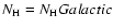 for the GRBs with a best-fit
intrinsic
consistent with zero. The rightmost BeppoSAX curve
assumes for these GRBs the 90% upper limit. b), right panel, histograms of the Swift GRB with (shadow histogram) and without
redshift (black histogram).
for the GRBs with a best-fit
intrinsic
consistent with zero. The rightmost BeppoSAX curve
assumes for these GRBs the 90% upper limit. b), right panel, histograms of the Swift GRB with (shadow histogram) and without
redshift (black histogram). |
| Open with DEXTER | |
In the text
![\begin{figure}
\par\includegraphics[width=6.8cm,clip]{7157fig7.eps}
\end{figure}](/articles/aa/full/2007/29/aa7157-07/img23.gif) |
Figure 4: The R magnitude of the optical afterglow at the time of its discovery as a function of this time. Filled symbols are GRBs with reliable redshift determination. The size of the symbol is proportional to the redshift (the larger the symbol, the higher the redshift). Circles = Swift GRBs; squares = BeppoSAX GRBs; triangles = HETE2 GRBs. |
| Open with DEXTER | |
In the text
![\begin{figure}
\par\includegraphics[width=6.5cm,clip]{7157fig8.eps}\hspace*{3mm}
\includegraphics[width=6.5cm,clip]{7157fig9.eps}
\end{figure}](/articles/aa/full/2007/29/aa7157-07/img24.gif) |
Figure 5:
a), left panel, the distribution of the R magnitude 10ks
after the GRB events for the Swift (solid histogram) and the
BeppoSAX+HETE2 (dashed histogram) GRB samples. b), right panel, the
distribution of the  -ray (15-150 keV) to optical (R band) flux
ratio for the Swift (solid histogram), and BeppoSAX+HETE2 (red
histogram) GRB samples. -ray (15-150 keV) to optical (R band) flux
ratio for the Swift (solid histogram), and BeppoSAX+HETE2 (red
histogram) GRB samples. |
| Open with DEXTER | |
In the text
![\begin{figure}
\par\includegraphics[width=7.4cm,clip]{7157fig10.eps}\hspace*{4mm}
\includegraphics[width=7cm,clip]{7157fig11.eps}
\end{figure}](/articles/aa/full/2007/29/aa7157-07/img28.gif) |
Figure 6:
The redshift as a function of the 15-150 keV peak flux a),
left panel, and of the observer frame
b),
right panel, for the
Swift (circles), BeppoSAX (triangles) and HETE2 (squares) GRBs. GRB
without a measured redshift are plotted at a constant z as empty
symbols. The left dashed line in Fig. 6b is the
expectation for a constant, rest-frame column density of
 ,
and the right dashed line is the expectation for ,
and the right dashed line is the expectation for
 . . |
| Open with DEXTER | |
In the text
![\begin{figure}
\par\includegraphics[width=7cm,clip]{7157fig12.eps}
\end{figure}](/articles/aa/full/2007/29/aa7157-07/img47.gif) |
Figure 7:
The average cumulative redshift distribution of a subsample
of Swift GRBs having the same peak flux,
and R mag (at 10 ks)
distributions of the joined BeppoSAX+HETE2 samples (thin solid line)
compared with the Swift (thick solid line) and BeppoSAX+HETE2 (dashed
line) total redshift distributions. The thin dotted lines mark the
redshift range covered by 100 random extractions and give an idea
of the statistical uncertainty associated to a single extraction of a
redshift distribution of 26 GRBs from a parent population. |
| Open with DEXTER | |
In the text