A&A 470, 39-51 (2007)
DOI: 10.1051/0004-6361:20077245

Substructures in WINGS clusters

M. Ramella¹ - A. Biviano¹ - A. Pisani² - J. Varela^3,8 - D. Bettoni³ - W. J. Couch⁴ - M. D'Onofrio⁵ - A. Dressler⁶ - G. Fasano³ - P. Kjærgaard⁷ - M. Moles⁸ - E. Pignatelli³ - B. M. Poggianti³

1 - INAF/Osservatorio Astronomico di Trieste, via G. B. Tiepolo 11, 34143 Trieste, Italy
2 - Istituto di Istruzione Statale Classico Dante Alighieri, Scientifico Duca degli Abruzzi, Magistrale S. Slataper, viale XX settembre 11, 34170 Gorizia, Italy
3 - INAF/Osservatorio Astronomico di Padova, vicolo Osservatorio 5, 35122 Padova, Italy
4 - School of Physics, University of New South Wales, Sydney 2052, Australia
5 - Dipartimento di Astronomia, Università di Padova, vicolo Osservatorio 2, 35122 Padova, Italy
6 - Observatories of the Carnegie Institution of Washington, Pasadena, CA 91101, USA
7 - Copenhagen University Observatory. The Niels Bohr Institute for Astronomy Physics and Geophysics, Juliane Maries Vej 30, 2100 Copenhagen, Denmark
8 - Instituto de Astrofísica de Andalucía (C.S.I.C.) Apartado 3004, 18080 Granada, Spain

Received 6 February 2007 / Accepted 3 April 2007

Abstract
Aims. We search for and characterize substructures in the projected distribution of galaxies observed in the wide field CCD images of the 77 nearby clusters of the WIde-field Nearby Galaxy-cluster Survey (WINGS). This sample is complete in X-ray flux in the redshift range 0.04<z<0.07.
Methods. We search for substructures in WINGS clusters with DEDICA, an adaptive-kernel procedure. We test the procedure on Monte-Carlo simulations of the observed frames and determine the reliability for the detected structures.
Results. DEDICA identifies at least one reliable structure in the field of 55 clusters. 40 of these clusters have a total of 69 substructures at the same redshift of the cluster (redshift estimates of substructures are from color-magnitude diagrams). The fraction of clusters with subclusters (73%) is higher than in most studies. The presence of subclusters affects the relative luminosities of the brightest cluster galaxies (BCGs). Down to $L \sim 10^{11.2}~L_{\odot}$, our observed differential distribution of subcluster luminosities is consistent with the theoretical prediction of the differential mass function of substructures in cosmological simulations.

Key words: galaxies: clusters: general - galaxies: elliptical and lenticular, cD

1 Introduction

According to the current cosmological paradigm, large structures in the Universe form hierarchically. Clusters of galaxies are the largest structures that have grown through mergers of smaller units and have achieved near dynamical equilibrium. In the hierarchical scenario, clusters are a rather young population, and we should be able to observe their formation process even at rather low redshifts. A signature of such process is the presence of cluster substructures. A cluster is said to contain substructures (or subclusters) when its surface density is characterized by multiple, statistically significant peaks on scales larger than the typical galaxy size, with "surface density'' being referred to the cluster galaxies, the intra-cluster (IC) gas or the dark matter (DM hereafter; Buote 2002).

Studying cluster substructure therefore allows us to investigate the process by which clusters form, constrain the cosmological model of structure formation, and ultimately test the hierarchical paradigm itself (e.g. Thomas et al. 1998; Richstone et al. 1992; Mohr et al. 1995). In addition, it also allows us to better understand the mechanisms affecting galaxy evolution in clusters, which can be accelerated by the perturbative effects of a cluster-subcluster collision and of the tidal field experienced by a group accreting onto a cluster (Dubinski 1999; Bekki 1999; Gnedin 1999). If clusters are to be used as cosmological tools, it is important to calibrate the effects substructures have on the estimate of their internal properties (e.g. Roettiger et al. 1998; Lopes et al. 2006; Schindler & Müller 1993; Biviano et al. 2006; Pinkney et al. 1996). Finally, detailed analyses of cluster substructures can be used to constrain the nature of DM (Markevitch et al. 2004; Clowe et al. 2006).

The analysis of cluster substructures can be performed using the projected phase-space distribution of cluster galaxies (e.g. Geller & Beers 1982), the surface-brightness distribution and temperature of the X-ray emitting IC gas (e.g. Briel et al. 1992), or the shear pattern in the background galaxy distribution induced by gravitational lensing, that directly samples substructure in the DM component (e.g. Abdelsalam et al. 1998). None of these tracers of cluster substructure (cluster galaxies, IC gas, background galaxies) can be considered optimal. The identification of substructures is in fact subject to different biases depending on the tracer used. In X-rays projection effects are less important than in the optical, but the identification of substructures is more subject to a z-dependent bias, arising from the point spread function of the X-ray telescope and detector (e.g. Böhringer & Schuecker 2002). Moreover, the different cluster components respond in a different way to a cluster-subcluster collision. The subcluster IC gas can be ram-pressure braked and stripped from the colliding subcluster and lags behind the subcluster galaxies and DM along the direction of collision (e.g. Clowe et al. 2006; Barrena et al. 2002; Roettiger et al. 1997). Hence, it is equally useful to address cluster substructure analysis in the X-ray and in the optical.

Traditionally, the first detections of cluster substructures were obtained from the projected spatial distributions of galaxies (e.g. Shane & Wirtanen 1954; Abell et al. 1964), in combination, when possible, with the distribution of galaxy velocities (e.g. van den Bergh 1960; de Vaucouleurs 1961; van den Bergh 1961). Increasingly sophisticated techniques for the detection and characterization of cluster substructures have been developed over the years (see Girardi & Biviano 2002; Perea et al. 1986b; Moles et al. 1986; Perea et al. 1986a; Buote 2002, and references therein). In many of these techniques substructures are identified as deviations from symmetry in the spatial and/or velocity distribution of galaxies and in the X-ray surface-brightness (e.g. Mohr et al. 1993; Fitchett & Merritt 1988; Schuecker et al. 2001; West et al. 1988). In other techniques substructures are identified as significant peaks in the surface density distribution of galaxies or in the X-ray surface brightness, either as residuals left after the subtraction of a smooth, regular model representation of the cluster (e.g. Ettori et al. 1998; Neumann & Böhringer 1997), or in a non-parametric way, e.g. by the technique of wavelets (e.g. Biviano et al. 1996; Slezak et al. 1994; Escalera et al. 1994) and by adaptive-kernel techniques (e.g. Bardelli et al. 2001,1998a; Kriessler & Beers 1997).

The performances of several different methods have been evaluated both using numerical simulations (e.g. Crone et al. 1996; Cen 1997; Valdarnini et al. 1999; Knebe & Müller 2000; Biviano et al. 2006; Buote & Xu 1997; Mohr et al. 1995; Pinkney et al. 1996) and also by applying different methods to the same cluster data-sets and examine the result differences (e.g. Mohr et al. 1996; Fadda et al. 1998; Escalera et al. 1992; Lopes et al. 2006; Kriessler & Beers 1997; Escalera et al. 1994; Kolokotronis et al. 2001; Mohr et al. 1995; Schuecker et al. 2001). Generally speaking, the sensitivity of substructure detection increases with both increasing statistics (e.g. more galaxies or more X-ray photons) and increasing dimensionality of the test (e.g. using galaxy velocities in addition to their positions, or using X-ray temperature in addition to X-ray surface brightness).

Previous investigations have found very different fractions of clusters with substructure in nearby clusters, depending on the method and tracer used for substructure detection, on the cluster sample, and on the size of sampled cluster regions (e.g. Flin & Krywult 2006; Lopes et al. 2006; Girardi et al. 1997; Solanes et al. 1999; Kriessler & Beers 1997; Jones & Forman 1999; Dressler & Shectman 1988; Geller & Beers 1982; Kolokotronis et al. 2001; Mohr et al. 1995; Schuecker et al. 2001). Although the distribution of subcluster masses has not been determined observationally, it is known that subclusters of $\sim$10% the cluster mass are typical, while more massive subclusters are less frequent (Jones & Forman 1999; Girardi et al. 1997; Escalera et al. 1994). The situation is probably different for distant clusters which tend to show massive substructures more often than nearby clusters clearly suggesting hierarchical growth of clusters was more intense in the past (e.g. Gioia et al. 1999; Demarco et al. 2005; Rosati et al. 2004; Maughan et al. 2003; van Dokkum et al. 2000; Haines et al. 2001; Huo et al. 2004; Jeltema et al. 2005).

Additional evidence for the hierarchical formation of clusters is provided by the analysis of brightest cluster galaxies (BCGs hereafter) in substructured clusters. BCGs usually sit at the bottom of the potential well of their host cluster (e.g. Adami et al. 1998b). When a BCG is found to be significantly displaced from its cluster dynamical center, the cluster displays evidence of substructure (e.g. Beers et al. 1991; Ferrari et al. 2006). From the correlation between cluster and BCG luminosities, Lin & Mohr (2004) conclude that BCGs grow by merging as their host clusters grow hierarchically. The related evolution of BCGs and their host clusters is also suggested by the alignment of the main cluster and BCG axes (e.g. Binggeli 1982; Durret et al. 1998). Both the BCG and the cluster axes are aligned with the surrounding large scale structure distribution, where infalling groups come from. These infalling groups are finally identified as substructures once they enter the cluster environment (West & Blakeslee 2000; Adami et al. 2005; Ferrari et al. 2003; Durret et al. 1998; Plionis et al. 2003; Arnaud et al. 2000). Hence, substructure studies really provide direct evidence for the hierarchical formation of clusters.

Concerning the impact of subclustering on global cluster properties, it has been found that subclustering leads to over-estimating cluster velocity dispersions and virial masses (e.g. Bird 1995; Maurogordato et al. 2000; Perea et al. 1990), but not in the general case of small substructures (Xu et al. 2000; Girardi et al. 1997; Escalera et al. 1994). During the collision of a subcluster with the main cluster, both the X-ray emitting gas distribution and its temperature have been found to be significantly affected (e.g. Markevitch & Vikhlinin 2001; Clowe et al. 2006). As a consequence, it has been argued that substructure can explain at least part of the scatter in the scaling relations of optical-to-X-ray cluster properties (e.g. Girardi et al. 1996; Lopes et al. 2006; Barrena et al. 2002; Fitchett 1988).

As far as the internal properties of cluster galaxies are concerned, there is observational evidence that a higher fraction of cluster galaxies with spectral features characteristic of recent or ongoing starburst episodes is located in substructures or in the regions of cluster-subcluster interactions (Bardelli et al. 1998b; Miller 2005; Caldwell et al. 1993; Poggianti et al. 2004; Moss & Whittle 2000; Miller et al. 2004; Abraham et al. 1996; Biviano et al. 1997; Giacintucci et al. 2006; Caldwell & Rose 1997).

In this paper we search for and characterize substructures in the sample of 77 nearby clusters of the WIde-field Nearby Galaxy-cluster Survey (WINGS hereafter, Fasano et al. 2006). This sample is an almost complete sample in X-ray flux in the redshift range 0.04<z<0.07. We detect substructures from the spatial, projected distribution of galaxies in the cluster fields, using the adaptive-kernel based DEDICA algorithm (Pisani 1996,1993). In Sect. 2 we describe our data-set; in Sect. 3 we describe the procedure of substructure identification; in Sect. 4 we use Monte Carlo simulations in order to tweak our procedure; in Sect. 5 we describe the identification of substructures in our data-set; in Sect. 6 the catalog of identified substructures is provided. In Sect. 7 we investigate the properties of the identified substructures, and in Sect. 8 we consider the relation between the BCGs and the substructures. We provide a summary of our work in Sect. 9.

   
2 The data

WINGS is an all-sky, photometric (multi-band) and spectroscopic survey, whose global goal is the systematic study of the local cosmic variance of the cluster population and of the properties of cluster galaxies as a function of cluster properties and local environment.

The WINGS sample consists of 77 clusters selected from three X-ray flux limited samples compiled from ROSAT All-Sky Survey data, with constraints just on the redshift (0.04 < z < 0.07) and distance from the galactic plane ( ${\vert}b{\vert}$ $\geq$ 20 deg). The core of the project consists of wide-field optical imaging of the selected clusters in the B and V bands. The imaging data were collected using the WFC@INT (La Palma) and the WFI@MPG/ESO2.2 (La Silla) in the northern and southern hemispheres, respectively.

The observation strategy of the survey favors the uniformity of photometric depth inside the different CCDs, rather than complete coverage of the fields that would require dithering. Thus, the gaps in the WINGS optical imaging correspond to the physical gaps between the different CCDs of the mosaics.

During the data reduction process, we give particular care to sky subtraction (also in presence of crowded fields including big halo galaxies and/or very bright stars), image cleaning (spikes and bad pixels) and star/galaxy classification (obtained with both automatic and interactive tools).

According to Fasano et al. (2006) and Varela et al. (2007), the overall quality of the data reported in the WINGS photometric catalogs can be summarized as follows: (i) the astrometric errors for extended objects have ${\rm rms} \sim$ 0.2 arcsec; (ii) the average limiting magnitude is $\sim$24.0, ranging from 23.0 to 25.0; (iii) the completeness of the catalogs is achieved (on average) up to $V\sim$ 22.0; (iv) the total (systematic plus random) photometric rms errors, derived from both internal and external comparisons, vary from $\sim$0.02 mag, for bright objects, up to $\sim$0.2 mag, for objects close to the detection limit.

   
3 The DEDICA procedure

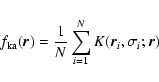
We base our search for substructures in WINGS clusters on the DEDICA procedure (Pisani 1996,1993). This procedure has the following advantages:

1.

DEDICA gives a total description of the clustering pattern, in particular the membership probability and significance of structures besides geometrical properties;

2.

DEDICA is scale invariant;

3.

DEDICA does not assume any property of the clusters, i.e. it is completely non-parametric. In particular it does not require particularly rich samples to run effectively.

The basic nature and properties of DEDICA are described in Pisani (1996, and references therein,1993). Here we summarize the main structure of the algorithm and how we apply it to our data sample. The core structure of DEDICA is based on the assumption that a structure (or a "cluster'' in the algorithm jargon) corresponds to a local maximum in the density of galaxies.

We proceed as follows. First we need to estimate the probability density function  $\Psi({\vec r}_{i})$ (with $i=1,\ldots N$) associated with the set of N galaxies with coordinates  ${\vec r}_{i}$. Second, we need to find the local maxima in our estimate of  $\Psi({\vec r}_{i})$ in order to identify clusters and also to evaluate their significance relatively to the noise. Third and finally, we need to estimate the probability that a galaxy is a member of the identified clusters.

   
3.1 The probability density

DEDICA is a non-parametric method in the sense that it does not require any assumption on the probability density function that it is aimed to estimate. The only assumptions are that  $\Psi({\vec r}_{i})$ must be continuous and at least twice differentiable.

The function $f({\vec r}_{i})$ is an estimate of $\Psi({\vec r}_{i})$ and it is built by using an adaptive kernel method given by:

$$% f_{\rm ka}({\vec r})=\frac{1}{N} \sum_{i=1}^{N} K({\vec r}_{i},\sigma_{i};{\vec r})$$ (1)

where we use the two dimensional Gaussian kernel $K({\vec r}_{i},\sigma_{i};{\vec r})$ centered in ${\vec r}_{i}$ with size $\sigma_{i}$.

The most valuable feature of DEDICA is the procedure to select the values of kernel widths  $\sigma_{i}$. It is possible to show that the optimal choice for  $\sigma_{i}$, i.e. with asymptotically minimum variance and null bias, is obtained by minimizing the distance between our estimate $f({\vec r}_{i})$ and  $\Psi({\vec r}_{i})$. This distance can be evaluated by a particular function called the integrated square error  ${\it ISE}(f)$ given by:

$$% {\it ISE}(f)=\int_{\Re} [\Psi({\vec r}) - f({\vec r})]^2 {\rm d}{\vec r}.$$ (2)

Once the minimum ${\it ISE}(f)$ is reached we have obtained the DEDICA estimate of the density as in Eq. (1).

   
3.2 Cluster identification

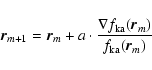
The second step of DEDICA consists in the identification of the local maxima in $f_{\rm ka}({\vec r})$. The positions of the peaks in the density function  $f_{\rm ka}({\vec r})$ are found as the solutions of the iterative equation:

$$% {\vec r}_{m+1}={\vec r}_{m} +a \cdot \frac{\nabla f_{\rm ka}({\vec r}_m)}{f_{\rm ka}({\vec r}_m)}$$ (3)

where a is a scale factor set according to optimal convergence requirements. The limit ${\vec R}$ of the sequence  ${\vec r}_m$ defined in Eq. (3) depends on the starting position ${\vec r}_{m=1}$.

$$% \lim_{m \rightarrow + \infty} {\vec r}_{m}= {{\vec R}}( {\vec r}_{m=1}) .$$ (4)

We run the sequence in Eq. (3) at each data position  ${\vec r}_{i}$. We label each data point with the limit  ${{\vec R}}_i={{\vec R}}({\vec r}_{m=1}={\vec r}_{i})$. These limits  ${\vec R}_i$ are the position of the peak to which the ith galaxy belong. In the case that all the galaxies are members of a unique cluster, all the labels  ${\vec R}_i$ are the same. At the other extreme each galaxy is a one-member cluster and all ${\vec R}_i$ have different values. All the members of a given cluster belong to the same peak in $f_{\rm ka}({\vec r})$ and have the same ${\vec R}_i$. We identify cluster members by listing galaxies having the same values of ${\vec R}$. We end up with $\nu$ different clusters each with $n_{\mu}$ ( $\mu=1, \ldots, \nu$) members.

In order to maintain a coherent notation, we identify with the label $\mu=0$the n₀ isolated galaxies considered a system of background galaxies. We have: $n_0 = N- \sum_{\mu=1}^{\nu} n_\mu$.

   
3.3 Cluster significance and membership probability

The statistical significance $S_\mu$ ( $\mu=1, \ldots, \nu$) of each cluster is based on the assumption that the presence of the $\mu$th cluster causes an increase in the local probability density as well as in the sample likelihood $L_N = \Pi_i [ f_{\rm ka}({\vec r}_i) ]$ relatively to the value $L_\mu$ that one would have if the members of the $\mu$th cluster were all isolated, i.e. belonging to the background.

A large value in the ratio $L_N / L_\mu$ characterizes the most important clusters. According to Materne (1979) it is possible to estimate the significance of each cluster by using the likelihood ratio test. In other words $2 \ln (L_N / L_\mu)$ is distributed as a $\chi^2$ variable with $\nu-1$ degrees of freedom. Therefore, once we compute the value of $\chi^2$ for each cluster ( $\chi ^2_{\rm S}$), we can also compute the significance $S_\mu$ of the cluster.

Here we assume that the contribution to the global density field  $f_{\rm ka}({\vec r}_i)$ of the $\mu$th cluster is $F_\mu({\vec r}_i)$. The ratio between the value of  $F_\mu({\vec r}_i)$ and the total local density  $f_{\rm ka}({\vec r}_i)$ can be used to estimate the membership probability of each galaxy relatively to the identified clusters. This criterion also allows us to estimate the probability that a galaxy is isolated.

At the end of the DEDICA procedure we are left with a) a catalog of galaxies each with information on position, membership, local density and size of the Gaussian kernel, b) a catalog of structures with information on position, richness, the $\chi ^2_{\rm S}$ parameter, and peak density. For each cluster we also compute from the coordinate variance matrix, the cluster major axis, ellipticity and position angle.

   
4 Tweaking the algorithm with simulations

In this section we describe our analysis of the performance of DEDICA and the guidelines we obtain for the interpretation of the clustering analysis of our observations.

We build simulated fields containing a cluster with and without subclusters. The simulated fields have the same geometry of the WFC field and are populated with the typical number of objects we will analyze. For simplicity we consider only WFC fields. Because DEDICA is scale-free, a different sampling of the same field of view has no consequence on our analysis.

In the next section we limit our analysis to $M_{V,{\rm lim}} \leq -16$. At the median redshift of the WINGS cluster, $z \simeq 0.05$, this absolute magnitude limit corresponds to an apparent magnitude $V_{\rm lim} \simeq 21$. Within this magnitude limit the representative number of galaxies in our frames is $N_{{\rm tot}}$ = 900.

We then consider $N_{{\rm tot}}$ = $N_{{\rm mem}}$ + $N_{{\rm bkg}}$, with $N_{{\rm mem}}$ the number of cluster members and  $N_{{\rm bkg}}$ the number of field - or background - galaxies. We set $N_{{\rm bkg}}$ = 670, close to the average number of background galaxies we expect in our frame based on typical observed fields counts, e.g. Berta et al. (2006) or Arnouts et al. (1997). With this choice, we have $N_{{\rm mem}}$ = 230.

We distribute uniformly at random $N_{{\rm bkg}}$ objects. We distribute at random the remaining $N_{{\rm mem}}$ = 230 objects in one or more overdensities depending on the test we perform. We populate overdensities according to a King profile (King 1962) with a core radius $R_{\rm core} = 90$ kpc, representative of our clusters. We then scale  $R_{\rm core}$ with the number of members of the substructure, $N_{\rm S}$. We use

$$\begin{eqnarray*}R_{\rm core} = 250 \sqrt{ \frac{N_{\rm S}}{N_{\rm C} + N_{\rm S}}} \end{eqnarray*}$$

where $N_{\rm C}$ is the number of objects in the cluster with $N_{{\rm mem}}$ = $N_{\rm S} + N_{\rm C}$. This scaling of  $R_{\rm core}$ with cluster richness is from Adami et al. (1998a) assuming direct proportionality between cluster richness and luminosity (e.g. Popesso et al. 2007).

As far as the relative richnesses of the cluster and subcluster are concerned, we consider the following richness ratios $r_{\rm cs} = N_{\rm C}/N_{\rm S} = 1, 2, 4, 8$. With these richness ratios, the number of objects in the cluster are $N_{\rm C} = 115, 153, 184, 204$, and those in subclusters are $N_{\rm S} = 115, 77, 46, 26$ respectively.

In a first set of simulated fields we place the substructure at 2731 pixels (15 arcmin) from the main cluster so that they do not overlap. In a second set of simulations, we place main cluster and substructure at shorter distances, 683 and 1366 pixels, in order to investigate the ability of DEDICA to resolve structures. At each of these shorter distances we build simulations with both $r_{{\rm cs}}$ = 1 and 2.

For each richness ratio and/or distance between cluster and subcluster we produce 16 simulations with different realizations of the random positions of the data points representing galaxies.

In order to minimize the effect of the borders on the detection of structures we add to the simulation a "frame'' of 1000 pixel. We fill this frame with a grid of data points at the same density as the average density of the field.

The first result we obtain from the runs of DEDICA on the simulations with varying richness ratio is the positive rate at which we detect real structures. We find that we always recover both cluster and substructure even when the substructure only contains $N_{\rm S}$ = 1/8 $N_{\rm C}$ objects, i.e. 26 objects (on top of the uniform background). In other words, if there is a real structure DEDICA finds it.

We also check how many original members the procedure assigns to structures it recovers. The results are summarized in Fig. 1. In the diagram, the fraction of recovered members of each substructure is represented by the values of its  $r_{{\rm cs}}$. The solid line connects substructures with $r_{\rm cs}=2$ and 4.

	Figure 1: Fraction of recovered members of each substructure for different  $r_{{\rm cs}}$. The solid line connects substructures with $r_{{\rm cs}}$ = 2 and 4.
Open with DEXTER

From Fig. 1 it is clear that our procedure recovers a large fraction of members, almost irrespective of the richness of the original structure. It is also interesting to note that the fluctuations identified as substructures are located very close to the center of the corresponding simulated substructures. In almost all cases the distance between original and detected substructure is significantly shorter than the mean inter-particle distance.

The second important result we obtain from the simulations is the false positive rate, i.e. the fraction of noise fluctuations that are as significant as the fluctuations corresponding to real structures.

First of all we need to define an operative measure of the reliability of the detected structures. In fact DEDICA provides a default value $S_\mu$ ( $\mu=1, \ldots, \nu$) of the significance (see Sect. 3.3). However, $S_\mu$ has a relatively small dynamical range, in particular for highly significant clusters.

Density or richness both allow a reasonable "ranking'' of structures. However, both large low-density noise fluctuations (often built up from more than one noise fluctuation) and very high density fluctuations produced by few very close data points could be mistakenly ranked as highly significant structures according to, respectively, richness and density criteria.

We therefore prefer to use the parameter $\chi ^2_{\rm S}$ which stands at the base of the estimate of $S_\mu$ and which is naturally provided by DEDICA. The main characteristic of $\chi ^2_{\rm S}$ is that it depends both on the density of a cluster relative to the background and on its richness. Using $\chi ^2_{\rm S}$ we classify correctly significantly more structures than with either density or richness alone.

	Figure 2: $\chi ^2_{\rm S}$ of simulated noise fluctuations (solid line). Labels are the $r_{{\rm cs}}$ of simulated structures at the abscissa corresponding to their $\chi ^2_{\rm S}$ and at arbitrary ordinates.
Open with DEXTER

In Fig. 2 we plot the distribution of $\chi ^2_{\rm S}$ of noise fluctuations (solid line). In the same plot we also mark the $r_{{\rm cs}}$ of real structures as detected by our procedure. We use labels indicating $r_{{\rm cs}}$ and place them at the abscissa corresponding to their $\chi ^2_{\rm S}$ and at arbitrary ordinates.

Figure 2 shows that the structures detected with $r_{{\rm cs}}$ = 1, 2 are always distinguishable from noise fluctuations. Substructures with $r_{{\rm cs}}$ = 4 or higher, although correctly detected, have $\chi ^2_{\rm S}$ values that are close to or lower than the level of noise.

With the second set of simulations, we test the minimum distance at which cluster and subcluster can still be identified as separate entities. We place cluster and substructure ( $r_{{\rm cs}}$ = 1, 2) at distances $d_{\rm cs} =$ 683 and 1366 pixel. These distances are 1/4 and 1/2 respectively of the distance between cluster and substructure in the first set of simulations. Again we produce 16 simulations for each of the 4 cases.

We find that at $d_{\rm cs} =$ 1366 pixel cluster and substructure are always correctly identified. At the shorter distance $d_{\rm cs} =$ 683 pixel, DEDICA merges cluster and substructure in 1 out of 16 cases for $r_{{\rm cs}}$ = 1 and in 8 out of 16 cases for $r_{{\rm cs}}$ = 2. With our density profile, $d_{\rm cs} =$ 683 pixel corresponds to $d_{\rm cs} \simeq R_{\rm c} + R_{\rm s}$ with $R_{\rm c}$, $R_{\rm s}$ the radii of the main cluster and of the subcluster respectively.

In order to verify the results we obtain for 900 data points we produce more simulations with $N_{{\rm tot}}$ = 450, 600 and 1200. In all these simulations $R_{\rm C}$ and $R_{\rm S}$ are the same as in the set with $N_{{\rm tot}}$ = 900. We vary $N_{{\rm bkg}}$ and $N_{{\rm mem}}$ so that $N_{{\rm mem}}$/ $N_{{\rm bkg}}$ is the same as in the case $N_{{\rm tot}}$ = 900.

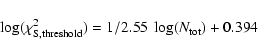
These simulations confirm the results we obtain in the case $N_{{\rm tot}}$ = 900, and allow us to set a detection threshold, $\chi ^2_{{\rm S,threshold}}$( $N_{{\rm tot}}$), for significant fluctuations in the analysis of real clusters.

We summarize the behavior of the noise fluctuations in our simulations in Fig. 3. In this figure, the small symbols correspond to $\chi ^2_{\rm S}$ as a function of the number of members of noise fluctuations. In particular, crosses, circles, dots and triangles are $\chi ^2_{\rm S}$ for the noise fluctuations of the simulations with $N_{{\rm tot}}$ = 450, 600, 900, and 1200 respectively.

The larger symbols are the $\chi ^2_{\rm S}$ of the fluctuations corresponding to simulated clusters and subclusters of equal richness ( $r_{{\rm cs}}$ = 1).

The 4 horizontal lines mark the level of $\chi ^2_{{\rm S,threshold}}$, i.e. the average $\chi ^2_{\rm S}$ of the 3 most significant noise fluctuations in each of the 4 groups of simulations with $N_{{\rm tot}}$ = 450, 600, 900, and 1200.

The expected increase of $\chi ^2_{{\rm S,threshold}}$ with $N_{{\rm tot}}$ is evident.

We note that the only significant difference with these findings we obtain from the simulations with $r_{{\rm cs}}$ = 2 is that $\chi ^2_{\rm S}$ of simulated clusters and subclusters is closer to $\chi ^2_{{\rm S,threshold}}$ (but still higher).

Figure 3: Small symbols correspond to $\chi ^2_{\rm S}$ as a function of the number of members of noise fluctuations. Crosses, circles, dots and triangles are $\chi ^2_{\rm S}$ for the noise fluctuations of the simulations with $N_{{\rm tot}}$ = 450, 600, 900, and 1200 respectively. Large symbols are $\chi ^2_{\rm S}$ of simulated clusters and subclusters with $r_{{\rm cs}}$ = 1. Horizontal lines mark the levels of $\chi ^2_{{\rm S,threshold}}$.

Open with DEXTER

We fit $\chi ^2_{{\rm S,threshold}}$ with $N_{{\rm tot}}$ and obtain

$$% \log(\chi^2_{\rm S,threshold}) = 1/2.55 ~ \log(N_{\rm tot}) + 0.394$$ (5)

in good agreement with the expected behavior of the poissonian fluctuations.

As a final test we verify that infra-chip gaps do not have a dramatic impact on the detection of structures in the cases $r_{{\rm cs}}$ = 1 and 2. We place a 50 pixel wide gap where it has the maximum impact, i.e. where the kernel size is shortest. Even if the infra-chip gap cuts through the center of the structures, DEDICA is able to identify these structures correctly.

We summarize here the main results of our tests on simulated clusters with substructures:

• DEDICA successfully detects even the poorest structures above a uniform poissonian noise background.

• DEDICA recovers a large fraction (typically >3/4) of the real members of a substructure, almost irrespective of the richness of the structure.

• DEDICA is able to distinguish between noise fluctuations and true structures only if these structures are rich enough. In the case of our simulations, structures have to be richer than 1/4th of the main structure.

• DEDICA is able to separate neighboring structures provided they do not overlap.

• infra-chip gaps do not threaten the detection of structures that are rich enough to be reliably detected.

• the $\chi ^2_{\rm S}$ threshold we use to identify significant structures is a function of the total number of points and can be scaled within the whole range of numbers of galaxies observed within our fields.

In the next section we apply these results to the real WINGS clusters.

   
5 Substructure detection in WINGS clusters

We apply our clustering procedure to the 77 clusters of the WINGS sample. The photometric catalog of each cluster is deep, reaching a completeness magnitude $V_{\rm complete} \leq 22$. The number of galaxies is correspondingly large, from $N_{\rm gal} \simeq 3000$ to $N_{\rm gal} \simeq 10~000$.

The large number of bright background galaxies (faint apparent magnitudes) dilutes the clustering signal of local WINGS clusters. We perform test runs of the procedure on several clusters with magnitude cuts brighter than  $V_{\rm complete}$. Based on these tests, we decide to cut galaxy catalogs to the absolute magnitude threshold M_V = -16.0. With this choice a) we maximize the signal-to-noise ratio of the detected subclusters and b) we still have enough galaxies for a stable identification of the system. At the median redshift of WINGS clusters, $z \simeq 0.05$, our absolute magnitude cut corresponds to an apparent magnitude $V \simeq 21$.

This apparent magnitude also approximately corresponds to the magnitude where the contrast of our typical cluster relative to the field is maximum (this estimate is based on the average cluster luminosity function of Yagi et al. (2002), De Propris et al. (2003) and on the galaxy counts of Berta et al. (2006)).

The number of galaxies that are brighter than the threshold M_V = -16.0 is in the range $600 < N_{\rm tot} < 1200$ for a large fraction of clusters observed with either WFC@INT or with WFI@MPG/ESO2.2.

In order to proceed with the identification of significant structures within WINGS clusters, we need to verify that our simulations are sufficiently representative of the real cases. In practice we need to compare the observed distributions of $\chi ^2_{\rm S}$ values of noise fluctuations with the corresponding simulated distributions. In the observations it is impossible to identify individual fluctuations as noise. In order to have an idea of the distributions of $\chi ^2_{\rm S}$ of noise fluctuations we consider that our fields are centered on real clusters. As a consequence, on average, fluctuations in the center of the frames are more likely to correspond to real systems than those at the borders.

	Figure 4: $\chi ^2_{\rm S}$ distributions for border (thick solid histogram) and central (thick dashed histogram) observed fluctuations. The thin solid line is the normalized distribution of $\chi ^2_{\rm S}$ of the noise fluctuations in our simulations.
Open with DEXTER

We therefore consider separately the fluctuations within the central regions of the frames and all other fluctuations (borders). We define the central regions as the central 10% of WFC and WFI areas. We plot in Fig. 4 the two distributions. The thick solid histogram is for the border and the thick dashed histogram for the center of the frames. The difference between "noise'' and "signal'' is clear. In the same figure we also plot the normalized distribution of $\chi ^2_{\rm S}$ of the noise fluctuations in our simulations (thin solid line). The distributions of $\chi ^2_{\rm S}$ of the observed and simulated fluctuations are in reasonable agreement considering a) the simple model used for the simulations and that b) in the observations we can not exclude real low- $\chi ^2_{\rm S}$ structures among noise fluctuations. We conclude that for our clusters we can adopt the same reliability threshold $\chi ^2_{{\rm S,threshold}}$ we determine from our simulations (Eq. (5)).

   
6 The catalog of substructures

We detect at least one significant structure in 55 (71%) clusters. We find that 12 clusters (16%) have no structure above the threshold (undetected). In the case of another 10 (13%) clusters we find significant structures only at the border of the field of view. In absence of a detection in the center of the frame, we consider these border structures unrelated to the target cluster. We also verify that in the Color-Magnitude Diagram (CMD) these border structures are redder than expected given the redshift of the target cluster. We consider also these 10 clusters undetected.

Here we list the 22 undetected clusters: A0133, A0548b, A0780, A1644, A1668, A1983, A2271, A2382, A2589, A2626, A2717, A3164, A3395, A3490, A3497, A3528a, A3556, A3560, A3809, A4059, RX1022, Z1261.

We note that undetected clusters are real physical systems according to their x-ray selection. From an operative point of view, the fact that these clusters are not detected by DEDICA is the result of the division into too many structures of the total available clustering signal in the field (or of a too large fraction of the clustering signal going into border structures). Several physical situations could be at the origin of missed detections. One possibility is an excess of physical substructures of comparable richness. Another possibility is that these clusters are embedded in regions of the large scale structure that are highly clustered.

We do not try to recover these structures because they can not be prominent enough. Since our analysis is bidimensional, we can only detect and use confidently the most prominent structures. Redshifts are needed for a more detailed analysis of cluster substructures.

We list the 55 clusters with significant structures in Table A.1. We give, for each substructure: (1) the name of the parent cluster; (2) the classification of the structure as main (M), subcluster (S), or background (B) together with their order number; (3) right ascension (J2000), and (4) declination (J2000) in decimal degrees of the DEDICA peak; the parameters of the ellipse we obtain from the variance matrix of the coordinates of galaxies in the substructure, i.e. (5) major axis in arcminutes, (6) ellipticity, and (7) position angle in degrees; (8) luminosity (see the next section); (9)  $\chi ^2_{\rm S}$.

Figure 5: Isodensity contours (logarithmically spaced) of the Abell 85 field. The title lists the coordinates of the center. The orientation is East to the left, North to the top. Galaxies belonging to the systems detected by DEDICA are shown as dots of different colors. Black, light green, blue, red, magenta, dark green are for the main system and the subsequent substructures ordered as in Table A.1. Large symbols are for galaxies with $M_V \leq -17.0$ that lie where local densities are higher than the median local density of the structure the galaxy belongs to. Open symbols mark the positions of the first- and second-ranked cluster galaxies, BCG1 and BCG2 respectively. Similar plots for the 55 analysed clusters are available in the electronic version of this journal.

Open with DEXTER

We make available contour plots of the number density fields of all clusters in Fig. 6 of the electronic version of this journal. In Fig. 5 we show an example of these plots. Isodensity contours are drawn at ten logarithmic intervals. Galaxies belonging to the systems detected by DEDICA are shown as dots of different colors. We use large symbols for brighter galaxies ( $M_V \leq -17.0$) that lie where local densities are higher than the median local density of the structure the galaxy belongs to. We also mark with open symbols the positions of the first- and second-ranked cluster galaxies, BCG1 and BCG2 respectively. Color coding is black, light green, blue, red, magenta, dark green for the main system and the subsequent substructures ordered as in Table A.1.

We describe and analyze in detail our catalog in the next section.

   
7 Properties of substructures

The first problem we face in order to study the statistical and physical properties of substructures is to determine their association with the main structure. In fact, the main structure itself has to be identified among the structures detected by DEDICA in each frame.

In most cases it is easy to identify the main structure of a cluster since it is located at the center of the frame and it has a high  $\chi ^2_{\rm S}$. In two cases (A0168 and A1736) the choice of the main structure is complicated because there are several similar structures near the center of the frame. In these cases we select the main structure for its highest  $\chi ^2_{\rm S}$.

At this point we limit our analysis to members of the structure that a) have an absolute magnitude $M_V \leq -17$ (corrected for Galactic absorption) and that b) are in the upper half of the distribution of DEDICA-defined local galaxy densities of the system they belong to. The galaxy density threshold we apply allows us to separate adjacent structures whose definition becomes more uncertain at lower galaxy density levels. The magnitude cut increases the relative weight of the galaxies we use to evaluate the nature of structures in the CMD.

After having identified the main structure, we need to determine which structures in the field of view of a given cluster have to be considered background structures. We consider a structure a physical substructure (or subcluster) if its color-magnitude relation (CMR hereafter) is identical, within the errors, to the CMR of the main structure.

As a first step we define the color-magnitude relation (CMR) of the "whole cluster'', i.e. of galaxies in the main structure together with all other galaxies not assigned to any structure by DEDICA. We compute the (B - V) CMR of the Coma cluster from published data (Adami et al. 2006). Then we keep fixed the slope of the linear CMR of Coma and shift it to the mean redshift of the cluster.

In order to determine that the main structure and a substructure are at the same redshift, we evaluate the fraction of background (red) galaxies, $f_{\rm bg}$, that each structure has in the CMD. If these fractions are identical within the errors (Gehrels 1986), we consider the two structures to be at the same redshift.

In practice we determine $f_{\rm bg}$ by assigning to the background those galaxies of a structure that are redder than a line parallel to the CMR and vertically shifted (i.e. redwards) by 2.33 times the root-mean square of the colors of galaxies in the CMR. We note that the probability that a random variable is greater than 2.33 in a Gaussian distribution is only 1%.

The result of the selection of main structures and substructures is the following: 40 clusters have a total of 69 substructures at the same redshift as the main structure, only 15 clusters are left without substructures. A total of 35 systems are found in the background. Considering a) the number density of poor-to-rich clusters (Mazure et al. 1996; Zabludoff et al. 1993), b) the average luminosity function of clusters (De Propris et al. 2003; Yagi et al. 2002), c) the total area covered by the 55 cluster fields, and d) the limiting apparent magnitude corresponding to our absolute magnitude threshold M_V=-16.0, we expect to find $\sim$0.5 $\pm$ 0.2 background systems per cluster field, 28 $\pm$ 11 in total. This estimate is consistent with the 35 background systems we find.

The fraction of clusters with subclusters (73%) is higher than generally found in previous investigations (typically $\sim$$30\%$, see, e.g., Girardi & Biviano 2002; Flin & Krywult 2006; Lopes et al. 2006, and references therein). Even if we count all undetected clusters as clusters without substructures, this fraction only decreases to 52% (40/77). It is however acknowledged that the fraction of substructured clusters depends, among other factors, on the algorithm used to detect substructures, on the quality and depth of the galaxy catalog. For example Kolokotronis et al. (2001) using optical and X-ray data find that the fraction of clusters with substructures is $\geq$45%, Burgett et al. (2004) using a battery of tests detect substructures in 84% of the 25 clusters of their sample.

Having established the "global'' fraction of substructured clusters, we now investigate the degree of subclustering of individual clusters, i.e. the distribution of the number of substructures  $N_{\rm sub}$ we find in our sample.

We find 15 (27%) clusters without substructures; 22 (40%) clusters with $N_{\rm sub}$ = 1; 10 (18%) clusters with $N_{\rm sub}$ = 2; 6 (11%) clusters with $N_{\rm sub}$ = 3; and 2 (3%) clusters with $N_{\rm sub}$ = 4. We plot in the left panel of Fig. 7 the integral distribution of  $N_{\rm sub}$.

	Figure 7: Cumulative distributions of the two different indicators ofsubclustering: left panel $N_{\rm sub}$, right panel $f_{L{\rm sub}}$.
Open with DEXTER

The distribution of the level of subclustering does not change when we measure it as the fractional luminosity of subclusters, $f_{L{\rm sub}}$, relative to the luminosity of the whole cluster (see Fig. 7, right panel). The luminosities we estimate are background corrected using the counts of Berta et al. (2006). We use the ellipses output from DEDICA (see previous section) as a measure of the area of subclusters.

We find that $N_{\rm sub}$ and $f_{L{\rm sub}}$ are clearly correlated according to the Spearman rank-correlation test.

	Figure 8: Observed differential distribution of subcluster luminosities (histogram) and theoretical model (arbitrary scaling; De Lucia et al. 2004).
Open with DEXTER

We now consider the distribution of subcluster luminosities and plot the corresponding histogram in Fig. 8. In the same figure we also plot with arbitrary scaling the power-law $\propto$L^-1. This relation is the prediction for the differential mass function of substructures in the cosmological simulations of De Lucia et al. (2004).

Our observations are consistent to within the uncertainties with the theoretical prediction of De Lucia et al. (2004) down to $L \sim 10^{11.2}~L_{\odot}$. The disagreement at lower luminosity is expected since: a) below this limit galaxy-sized halos become important among the simulated substructures, and b) only above this limit we expect our catalog to be complete. In fact only subclusters with luminosities brighter than $L = 10^{11.2}~L_{\odot}$ have always richnesses that are $\geq$1/3 of the main structure. This richness limit approximately corresponds to the completeness limit of DEDICA detections according to our simulations (see Sect. 4).

   
8 Brightest cluster galaxies

Here we investigate the relation between BCGs and cluster structures.

We find that, on average, BCG1s are located close to the density peak of the main structures. In projection on the sky, the biweight average (see Beers et al. 1990) distance of BCG1s from the peak of the main system is 72 $\pm$ 11 kpc. If we only consider the 44 BCG1s that are on the CMR and are assigned to main systems by DEDICA, the average distance decreases to 56 $\pm$ 8 kpc. The fact that BCG1s are close to the center of the system is consistent with current theoretical view on the formation of BCGs (e.g. Dubinski 1998; Nipoti et al. 2004).

BCG2s are more distant than BCG1s from the peak of the main system: the biweight average distance is 345 $\pm$ 47 kpc. If we only consider the 26 BCG2s that are on the CMR and are assigned to main systems by DEDICA, the average distance decreases to 161 $\pm$ 34 kpc.

Projected distances of BCG2s from density peaks remain larger than those of BCG1s even when we consider the density peak of the structure or substructure they belong to. In Fig. 9 we plot the cumulative distributions of the distances of BCG1s (solid line) and BCG2s (dashed line) from the density peak of their systems. The distributions are different at the >99.99% level according to a Kolmogorov-Smirnov test (KS-test).

	Figure 9: Cumulative distributions of distances of BCG1 (solid line) and BCG2 (dashed line) from the density peak of their system.
Open with DEXTER

	Figure 10: Cumulative distributions of the magnitude difference between BCG1 and BCG2 in clusters with (dashed line) and without subclusters (solid line).
Open with DEXTER

Now we turn to luminosities and find that the magnitude difference between BCG1s and BCG2s, $\Delta M_{12}$, is larger in clusters without substructures than in clusters with substructures. In Fig. 10 we plot the cumulative distributions of  $\Delta M_{12}$ for clusters with (dashed line) and without (solid line) subclusters. The two distributions are different according to a KS-test at the 99.1% confidence level. We note that Lin & Mohr (2004) find that  $\Delta M_{12}$ is independent of cluster properties. These authors however do not consider subclustering.

In order to determine whether the higher values of  $\Delta M_{12}$ in clusters without subclusters are due to an increased luminosity of the BCG1 (L₁) or to a decreased luminosity of the BCG2 (L₂), we consider the luminosity of the 10th brightest galaxy (L₁₀) as a reference. The biweight average luminosity ratios are $\langle L_1/L_{10} \rangle$ = 8.6 $\pm$ 1.0 and $\langle L_2/L_{10} \rangle$ = 3.3 $\pm$ 0.3 in clusters without substructures, and $\langle L_1/L_{10} \rangle$ = 7.1 $\pm$ 0.4 and $\langle L_2/L_{10} \rangle$ = 3.4 $\pm$ 0.2 in clusters with substructures. We then conclude that the $\Delta M_{12}$-effect is caused by a brightening of the BCG1 relative to the BCG2 in clusters without substructures.

The fact that $\Delta M_{12}$ is higher in clusters without substructures can be interpreted, at least qualitatively, in the framework of the hierarchical scenario of structure evolution. Clusters without substructures are likely to be evolved after several merger phases. Their BCG1s have already had time to accrete many galaxies, in particular the more massive ones, which slow down and sink to the cluster center as the result of dynamical friction. Some of these galaxies may even have been BCGs of the merging structures. The simulations by De Lucia & Blaizot (2006) show that the BCG1s continue to increase their mass via cannibalism even at recent times, and that there is a large variance in the mass accretion history of BCG1s from cluster to cluster. The result of such a cannibalism process is an increase of the BCG1 luminosity with respect to other cluster galaxies, and in extreme cases may lead to the formation of fossil groups (Khosroshahi et al. 2006).

However, according to these simulations, only 15% of all BCG1s have accreted >30% of their mass over the last 2 Gyr, while another 15% have accreted <3% of their mass over the same period. Our results indicate that about 60% of the BCG1s are more than 1 mag brighter than the corresponding BCG2s. Given the size and generality of the luminosity differences it would seem that cannibalism alone, even if present along the merging history of a given cluster, cannot account for it. Most of the BCG1s should have then been assembled in early times, as pointed out in the downsizing scenario for galaxy formation (Cowie et al. 1996) and entered that merging history already with luminosity not far from the present one.

   
9 Summary

In this paper we search for and characterize cluster substructures, or subclusters, in the sample of 77 nearby clusters of the WINGS (Fasano et al. 2006). This sample is an almost complete sample in X-ray flux in the redshift range 0.04<z<0.07.

We detect substructures in the spatial projected distribution of galaxies in the cluster fields using DEDICA (Pisani 1996,1993) an adaptive-kernel technique. DEDICA has the following advantages for our study of WINGS clusters:

a)

DEDICA gives a total description of the clustering pattern, in particular membership probability and significance of structures besides geometrical properties.

b)

DEDICA is scale invariant

c)

DEDICA does not assume any property of the clusters, i.e. it is completely non-parametric. In particular it does not require particularly rich samples to run effectively.

In order to test DEDICA and to set guidelines for the interpretation of the results of the application of DEDICA to our observations we run DEDICA on several sets of simulated fields containing a cluster with and without subclusters.

We find that: a) DEDICA always identifies both cluster and subcluster even when the substructure richness ratio cluster-to-subcluster is $r_{{\rm cs}}$ = 8, b) DEDICA recovers a large fraction of members, almost irrespective of the richness of the original structure ($\ga$$70\%$ in most cases), c) structures with richness ratios $r_{{\rm cs}}$ $\la$ 3 are always distinguishable from noise fluctuations of the poissonian simulated field.

These simulations also allow us to define a threshold that we use to identify significant structures in the observed fields.

We apply our clustering procedure to the 77 clusters of the WINGS sample. We cut galaxy catalogs to the absolute magnitude threshold M_V = -16.0 in order to maximize the signal-to-noise ratio of the detected subclusters.

We detect at least one significant structure in 55 (71%) cluster fields. We find that 12 clusters (16%) have no structure above the threshold (undetected). In the remaining 10 (13%) clusters we find significant structures only at the border of the field of view. In absence of a detection in the center of the frame, we consider these border structures unrelated to the target cluster. We also verify that in the CMD these border structures are redder than expected given the redshift of the target cluster. We consider also these clusters undetected.

We provide the coordinates of all substructures in the 55 clusters together with their main properties.

Using the CMR of the early-type cluster galaxies we separate "true'' subclusters from unrelated background structures. We find that 40 clusters out of 55 (73%) have a total of 69 substructures with 15 clusters left without substructures.

The fraction of clusters with subclusters (73%) we identify is higher than most previously published values (typically $\sim$30%, see, e.g., Girardi & Biviano 2002, and references therein). It is however acknowledged that the fraction of substructured clusters depends, among other factors, on the algorithm used to detect substructures, on the quality and depth of the galaxy catalog (Burgett et al. 2004; Kolokotronis et al. 2001).

Another important result of our analysis is the distribution of subcluster luminosities. In the luminosity range where our substructure detection is complete ( $L \geq 10^{11.2}~L_{\odot}$), we find that the distribution of subcluster luminosities is in agreement with the power-law $\propto$L^-1 predicted for the differential mass function of substructures in the cosmological simulations of De Lucia et al. (2004).

Finally, we investigate the relation between BCGs and cluster structures.

We find that, on average, BCG1s are located close to the density peak of the main structures. In projection on the sky, the biweight average distance of BCG1s from the peak of the main system is 72 $\pm$ 11 kpc. BCG2s are significantly more distant than BCG1s from the peak of the main system (345 $\pm$ 47 kpc).

The fact that BCG1s are close to the center of the system is consistent with current theoretical view on the formation of BCGs (Dubinski 1998).

A more surprising result is that the magnitude difference between BCG1s and BCG2s, $\Delta M_{12}$, is significantly larger in clusters without substructures than in clusters with substructures. This fact may be interpreted in the framework of the hierarchical scenario of structure evolution (e.g. De Lucia & Blaizot 2006).

   
Appendix A: The catalog of substructures

Table A.1:

We provide here the catalog of substructures. In Table A.1 we give, for each substructure: (1) the name of the parent cluster; (2) the classification of the structure as main (M), subcluster (S), or background (B) together with their order number; (3) right ascension (J2000), and (4) declination (J2000) in decimal degrees of the DEDICA peak; the parameters of the ellipse we obtain from the variance matrix of the coordinates of galaxies in the substructure, i.e. (5) major axis in arcminutes, (6) ellipticity, and (7) position angle in degrees; (8) luminosity; (9)  $\chi ^2_{\rm S}$.

References

• Abdelsalam, H. M., Saha, P., & Williams, L. L. R. 1998, AJ, 116, 1541 [NASA ADS] [CrossRef] (In the text)
• Abell, G. O., Neyman, J., & Scott, E. L. 1964, AJ, 69, 529 [CrossRef]
• Abraham, R. G., Smecker-Hane, T. A., Hutchings, J. B., et al. 1996, ApJ, 471, 694 [NASA ADS] [CrossRef]
• Adami, C., Mazure, A., Biviano, A., Katgert, P., & Rhee, G. 1998a, A&A, 331, 493 [NASA ADS] (In the text)
• Adami, C., Mazure, A., Katgert, P., & Biviano, A. 1998b, A&A, 336, 63 [NASA ADS] (In the text)
• Adami, C., Biviano, A., Durret, F., & Mazure, A. 2005, A&A, 443, 17 [NASA ADS] [CrossRef] [EDP Sciences]
• Adami, C., Picat, J. P., Savine, C., et al. 2006, A&A, 451, 1159 [NASA ADS] [CrossRef] [EDP Sciences] (In the text)
• Arnaud, M., Maurogordato, S., Slezak, E., & Rho, J. 2000, A&A, 355, 461 [NASA ADS]
• Arnouts, S., de Lapparent, V., Mathez, G., et al. 1997, A&AS, 124, 163 [NASA ADS] [CrossRef] (In the text)
• Bardelli, S., Pisani, A., Ramella, M., Zucca, E., & Zamorani, G. 1998a, MNRAS, 300, 589 [NASA ADS]
• Bardelli, S., Zucca, E., Zamorani, G., Vettolani, G., & Scaramella, R. 1998b, MNRAS, 296, 599 [NASA ADS]
• Bardelli, S., Zucca, E., & Baldi, A. 2001, MNRAS, 320, 387 [NASA ADS]
• Barrena, R., Biviano, A., Ramella, M., Falco, E. E., & Seitz, S. 2002, A&A, 386, 816 [NASA ADS] [CrossRef] [EDP Sciences]
• Beers, T. C., Flynn, K., & Gebhardt, K. 1990, AJ, 100, 32 [NASA ADS] [CrossRef] (In the text)
• Beers, T. C., Gebhardt, K., Forman, W., Huchra, J. P., & Jones, C. 1991, AJ, 102, 1581 [NASA ADS] [CrossRef]
• Bekki, K. 1999, ApJ, 510, L15 [NASA ADS] [CrossRef]
• Berta, S., Rubele, S., Franceschini, A., et al. 2006, A&A, 451, 881 [NASA ADS] [CrossRef] [EDP Sciences] (In the text)
• Binggeli, B. 1982, A&A, 107, 338 [NASA ADS]
• Bird, C. M. 1995, ApJ, 445, L81 [NASA ADS] [CrossRef]
• Biviano, A., Durret, F., Gerbal, D., et al. 1996, A&A, 311, 95 [NASA ADS]
• Biviano, A., Katgert, P., Mazure, A., et al. 1997, A&A, 321, 84 [NASA ADS]
• Biviano, A., Murante, G., Borgani, S., et al. 2006, A&A, 456, 23 [NASA ADS] [CrossRef] [EDP Sciences]
• Böhringer, H., & Schuecker, P. 2002, Observational signatures and statistics of galaxy Cluster Mergers: Results from X-ray observations with ROSAT, ASCA, and XMM-Newton, Merging Processes in Galaxy Clusters, ASSL, 272, 133 (In the text)
• Briel, U. G., Henry, J. P., & Boehringer, H. 1992, A&A, 259, L31 [NASA ADS] (In the text)
• Buote, D. A. 2002, X-Ray Observations of Cluster Mergers: Cluster Morphologies and Their Implications, Merging Processes in Galaxy Clusters, ASSL, 272, 79 (In the text)
• Buote, D. A., & Xu, G. 1997, MNRAS, 284, 439 [NASA ADS]
• Burgett, W. S., Vick, M. M., Davis, D. S., et al. 2004, MNRAS, 352, 605 [NASA ADS] (In the text)
• Caldwell, N., & Rose, J. A. 1997, AJ, 113, 492 [NASA ADS] [CrossRef]
• Caldwell, N., Rose, J. A., Sharples, R. M., Ellis, R. S., & Bower, R. G. 1993, AJ, 106, 473 [NASA ADS] [CrossRef]
• Cen, R. 1997, ApJ, 485, 39 [NASA ADS] [CrossRef]
• Clowe, D., Bradac, M., Gonzalez, A. H., et al. 2006, ApJ, 648, L109 [NASA ADS] [CrossRef]
• Cowie, L. L., Songaila, A., Hu, E. M., & Cohen, J. G. 1996, AJ, 112, 839 [NASA ADS] [CrossRef] (In the text)
• Crone, M. M., Evrard, A. E., & Richstone, D. O. 1996, ApJ, 467, 489 [NASA ADS] [CrossRef]
• De Lucia, G., & Blaizot, J. 2006, ArXiv Astrophysics e-prints (In the text)
• De Lucia, G., Kauffmann, G., Springel, V., et al. 2004, MNRAS, 348, 333 [NASA ADS] (In the text)
• De Propris, R., Colless, M., Driver, S. P., et al. 2003, MNRAS, 342, 725 [NASA ADS] (In the text)
• de Vaucouleurs, G. 1961, ApJS, 6, 213 [NASA ADS] [CrossRef]
• Demarco, R., Rosati, P., Lidman, C., et al. 2005, A&A, 432, 381 [NASA ADS] [CrossRef] [EDP Sciences]
• Dressler, A., & Shectman, S. A. 1988, AJ, 95, 985 [NASA ADS] [CrossRef]
• Dubinski, J. 1998, ApJ, 502, 141 [NASA ADS] [CrossRef]
• Dubinski, J. 1999, in Galaxy Dynamics - A Rutgers Symposium, ed. D. R. Merritt, M. Valluri, & J. A. Sellwood, ASP Conf. Ser., 182, 491
• Durret, F., Forman, W., Gerbal, D., Jones, C., & Vikhlinin, A. 1998, A&A, 335, 41 [NASA ADS]
• Escalera, E., Slezak, E., & Mazure, A. 1992, A&A, 264, 379 [NASA ADS]
• Escalera, E., Biviano, A., Girardi, M., et al. 1994, ApJ, 423, 539 [NASA ADS] [CrossRef]
• Ettori, S., Fabian, A. C., & White, D. A. 1998, MNRAS, 300, 837 [NASA ADS]
• Fadda, D., Slezak, E., & Bijaoui, A. 1998, A&AS, 127, 335 [NASA ADS] [CrossRef]
• Fasano, G., Marmo, C., Varela, J., et al. 2006, A&A, 445, 805 [NASA ADS] [CrossRef] [EDP Sciences] (In the text)
• Ferrari, C., Maurogordato, S., Cappi, A., & Benoist, C. 2003, A&A, 399, 813 [NASA ADS] [CrossRef] [EDP Sciences]
• Ferrari, C., Arnaud, M., Ettori, S., Maurogordato, S., & Rho, J. 2006, A&A, 446, 417 [NASA ADS] [CrossRef] [EDP Sciences]
• Fitchett, M. J. 1988, in The Minnesota lectures on Clusters of Galaxies and Large-Scale Structure, ed. J. M. Dickey, ASP Conf. Ser., 5, 143
• Fitchett, M., & Merritt, D. 1988, ApJ, 335, 18 [NASA ADS] [CrossRef]
• Flin, P., & Krywult, J. 2006, A&A, 450, 9 [NASA ADS] [CrossRef] [EDP Sciences]
• Gehrels, N. 1986, ApJ, 303, 336 [NASA ADS] [CrossRef] (In the text)
• Geller, M. J., & Beers, T. C. 1982, PASP, 94, 421 [NASA ADS] [CrossRef] (In the text)
• Giacintucci, S., Venturi, T., Bardelli, S., et al. 2006, New Astron., 11, 437 [NASA ADS]
• Gioia, I. M., Henry, J. P., Mullis, C. R., Ebeling, H., & Wolter, A. 1999, AJ, 117, 2608 [NASA ADS] [CrossRef]
• Girardi, M., & Biviano, A. 2002, Optical Analysis of Cluster Mergers, Merging Processes in Galaxy Clusters, ASSL, 272, 39
• Girardi, M., Fadda, D., Giuricin, G., et al. 1996, ApJ, 457, 61 [NASA ADS] [CrossRef]
• Girardi, M., Escalera, E., Fadda, D., et al. 1997, ApJ, 482, 41 [NASA ADS] [CrossRef]
• Gnedin, O. Y. 1999, Ph.D. Thesis
• Haines, C. P., Clowes, R. G., Campusano, L. E., & Adamson, A. J. 2001, MNRAS, 323, 688 [NASA ADS]
• Huo, Z. Y., Xue, S. J., Xu, H., Squires, G., & Rosati, P. 2004, AJ, 127, 1263 [NASA ADS] [CrossRef]
• Jeltema, T. E., Canizares, C. R., Bautz, M. W., & Buote, D. A. 2005, ApJ, 624, 606 [NASA ADS] [CrossRef]
• Jones, C., & Forman, W. 1999, ApJ, 511, 65 [NASA ADS] [CrossRef]
• Khosroshahi, H. G., Ponman, T. J., & Jones, L. R. 2006, MNRAS, 372, L68 [NASA ADS] (In the text)
• King, I. 1962, AJ, 67, 471 [NASA ADS] [CrossRef] (In the text)
• Knebe, A., & Müller, V. 2000, A&A, 354, 761 [NASA ADS]
• Kolokotronis, V., Basilakos, S., Plionis, M., & Georgantopoulos, I. 2001, MNRAS, 320, 49 [NASA ADS]
• Kriessler, J. R., & Beers, T. C. 1997, AJ, 113, 80 [NASA ADS] [CrossRef]
• Lin, Y. T., & Mohr, J. J. 2004, ApJ, 617, 879 [NASA ADS] [CrossRef] (In the text)
• Lopes, P. A. A., de Carvalho, R. R., Capelato, H. V., et al. 2006, ApJ, 648, 209 [NASA ADS] [CrossRef]
• Markevitch, M., & Vikhlinin, A. 2001, ApJ, 563, 95 [NASA ADS] [CrossRef]
• Markevitch, M., Gonzalez, A. H., Clowe, D., et al. 2004, ApJ, 606, 819 [NASA ADS] [CrossRef]
• Materne, J. 1979, A&A, 74, 235 [NASA ADS] (In the text)
• Maughan, B. J., Jones, L. R., Ebeling, H., et al. 2003, ApJ, 587, 589 [NASA ADS] [CrossRef]
• Maurogordato, S., Proust, D., Beers, T. C., et al. 2000, A&A, 355, 848 [NASA ADS]
• Mazure, A., Katgert, P., den Hartog, R., et al. 1996, A&A, 310, 31 [NASA ADS]
• Miller, N. A. 2005, AJ, 130, 2541 [NASA ADS] [CrossRef]
• Miller, N. A., Owen, F. N., Hill, J. M., et al. 2004, ApJ, 613, 841 [NASA ADS] [CrossRef]
• Mohr, J. J., Fabricant, D. G., & Geller, M. J. 1993, ApJ, 413, 492 [NASA ADS] [CrossRef]
• Mohr, J. J., Evrard, A. E., Fabricant, D. G., & Geller, M. J. 1995, ApJ, 447, 8 [NASA ADS] [CrossRef]
• Mohr, J. J., Geller, M. J., Fabricant, D. G., et al. 1996, ApJ, 470, 724 [NASA ADS] [CrossRef]
• Moles, M., Perea, J., & del Olmo, A. 1986, MNRAS, 213, 365 [NASA ADS]
• Moss, C., & Whittle, M. 2000, MNRAS, 317, 667 [NASA ADS]
• Neumann, D. M., & Böhringer, H. 1997, MNRAS, 289, 123 [NASA ADS]
• Nipoti, C., Treu, T., Ciotti, L., & Stiavelli, M. 2004, MNRAS, 355, 1119 [NASA ADS]
• Perea, J., Moles, M., & del Olmo, A. 1986a, MNRAS, 219, 511 [NASA ADS]
• Perea, J., Moles, M., & del Olmo, A. 1986b, MNRAS, 222, 49 [NASA ADS]
• Perea, J., del Olmo, A., & Moles, M. 1990, A&A, 228, 310
• Pinkney, J., Roettiger, K., Burns, J. O., & Bird, C. M. 1996, ApJS, 104, 1 [NASA ADS] [CrossRef]
• Pisani, A. 1993, MNRAS, 265, 706 [NASA ADS]
• Pisani, A. 1996, MNRAS, 278, 697 [NASA ADS]
• Plionis, M., Benoist, C., Maurogordato, S., Ferrari, C., & Basilakos, S. 2003, ApJ, 594, 144 [NASA ADS] [CrossRef]
• Poggianti, B. M., Bridges, T. J., Komiyama, Y., et al. 2004, ApJ, 601, 197 [NASA ADS] [CrossRef]
• Popesso, P., Biviano, A., Böhringer, H., & Romaniello, M. 2007, A&A, 464, 451 [NASA ADS] [CrossRef] [EDP Sciences] (In the text)
• Richstone, D., Loeb, A., & Turner, E. L. 1992, ApJ, 393, 477 [NASA ADS] [CrossRef]
• Roettiger, K., Loken, C., & Burns, J. O. 1997, ApJS, 109, 307 [NASA ADS] [CrossRef]
• Roettiger, K., Stone, J. M., & Mushotzky, R. F. 1998, ApJ, 493, 62 [NASA ADS] [CrossRef]
• Rosati, P., Tozzi, P., Ettori, S., et al. 2004, AJ, 127, 230 [NASA ADS] [CrossRef]
• Schindler, S., & Müller, E. 1993, A&A, 272, 137 [NASA ADS]
• Schuecker, P., Böhringer, H., Reiprich, T. H., & Feretti, L. 2001, A&A, 378, 408 [NASA ADS] [CrossRef] [EDP Sciences]
• Shane, C. D., & Wirtanen, C. A. 1954, AJ, 59, 285 [NASA ADS] [CrossRef]
• Slezak, E., Durret, F., & Gerbal, D. 1994, AJ, 108, 1996 [NASA ADS] [CrossRef]
• Solanes, J. M., Salvador-Solé, E., & González-Casado, G. 1999, A&A, 343, 733 [NASA ADS]
• Thomas, P. A., Colberg, J. M., Couchman, H. M. P., et al. 1998, MNRAS, 296, 1061 [NASA ADS]
• Valdarnini, R., Ghizzardi, S., & Bonometto, S. 1999, New Astron., 4, 71 [NASA ADS]
• van den Bergh, S. 1960, MNRAS, 121, 387 [NASA ADS]
• van den Bergh, S. 1961, PASP, 73, 46 [NASA ADS] [CrossRef]
• van Dokkum, P. G., Franx, M., Fabricant, D., Illingworth, G. D., & Kelson, D. D. 2000, ApJ, 541, 95 [NASA ADS] [CrossRef]
• Varela, et al. 2007, A&A, submitted (In the text)
• West, M. J., & Blakeslee, J. P. 2000, ApJ, 543, L27 [NASA ADS] [CrossRef]
• West, M. J., Oemler, A. J., & Dekel, A. 1988, ApJ, 327, 1 [NASA ADS] [CrossRef]
• Xu, W., Fang, L. Z., & Wu, X. P. 2000, ApJ, 532, 728 [NASA ADS] [CrossRef]
• Yagi, M., Kashikawa, N., Sekiguchi, M., et al. 2002, AJ, 123, 87 [NASA ADS] [CrossRef] (In the text)
• Zabludoff, A. I., Geller, M. J., Huchra, J. P., & Ramella, M. 1993, AJ, 106, 1301 [NASA ADS] [CrossRef]

 

  
Online Material

Figure 6: Isodensity contours (logarithmically spaced) of the 55 clusters with significant structures. The title lists the coordinates of the center. The orientation is East to the left, North to the top. Galaxies belonging to the systems detected by DEDICA are shown as dots of different colors. Black, light green, blue, red, magenta, dark green are for the main system and the subsequent substructures ordered as in Table A.1. Large symbols are for galaxies with $M_V \leq -17.0$ that lie where local densities are higher than the median local density of the structure the galaxy belongs to. Open symbols mark the positions of the first- and second-ranked cluster galaxies, BCG1 and BCG2 respectively.

Open with DEXTER

	Figure 6: continued.
Open with DEXTER

	Figure 6: continued.
Open with DEXTER

	Figure 6: continued.
Open with DEXTER

	Figure 6: continued.
Open with DEXTER

	Figure 6: continued.
Open with DEXTER

	Figure 6: continued.
Open with DEXTER

	Figure 6: continued.
Open with DEXTER

	Figure 6: continued.
Open with DEXTER

	Figure 6: continued.
Open with DEXTER