A&A 470, 281-294 (2007)
DOI: 10.1051/0004-6361:20066500
L. Spezzi1,2,3 - J. M. Alcalá2 - A. Frasca1 - E. Covino2 - D. Gandolfi1,3
1 - INAF - Osservatorio Astrofisico di Catania, via S. Sofia 78, 95123 Catania, Italy
2 - INAF - Osservatorio Astronomico di Capodimonte, Salita Moiariello 16, 80131 Napoli, Italy
3 - Dipartimento di Fisica e Astronomia, Universitá di Catania, via S. Sofia 78, 95123 Catania, Italy
Received 3 October 2006 / Accepted 2 February 2007
Abstract
Aims. We present the results of an optical multi-band survey for low-mass pre-main sequence (PMS) stars and young brown dwarfs (BDs) in the Chamaeleon II (Cha II) dark cloud. This survey constitutes the complementary optical data to the c2d Spitzer Legacy survey in Cha II.
Methods. Using the wide-field imager (WFI) at the ESO 2.2 m telescope, we surveyed a sky area of about 1.75 square degrees in Cha II. The region was observed in the ![]() ,
,
![]() ,
and z broad-bands, in H
,
and z broad-bands, in H![]() and in two medium-band filters centred at 856 and 914 nm. We selected PMS star and young BD candidates using colour-magnitude diagrams (CMDs) and theoretical isochrones reproduced ad-hoc for the WFI at the ESO2.2m telescope system. We reinforced the selection criteria by using the previously known PMS stars in Cha II to define the PMS locus on the CMDs and by investigating the infrared (IR) colours of the candidates. By exploiting the WFI intermediate-band photometry we also estimated the effective temperature and the level of H
and in two medium-band filters centred at 856 and 914 nm. We selected PMS star and young BD candidates using colour-magnitude diagrams (CMDs) and theoretical isochrones reproduced ad-hoc for the WFI at the ESO2.2m telescope system. We reinforced the selection criteria by using the previously known PMS stars in Cha II to define the PMS locus on the CMDs and by investigating the infrared (IR) colours of the candidates. By exploiting the WFI intermediate-band photometry we also estimated the effective temperature and the level of H![]() emission of the candidates.
emission of the candidates.
Results. Our survey, which is one of the largest and deepest optical surveys conducted so far in Cha II, recovered the majority of the PMS stars and 10 member candidates of the cloud from previous IR surveys. In addition, the survey revealed 10 new potential members. From our photometric characterisation, we estimate that some 50% of the 20 candidates will result in true Cha II members. Based on our temperature estimates, we conclude that several of these objects are expected to be sub-stellar and give a first estimate of the fraction of sub-stellar objects.
Key words: stars: low-mass, brown dwarfs - stars: formation - stars: pre-main sequence - ISM: clouds - ISM: individual objects: Chamaeleon II
Recent investigations in star-forming regions (SFRs) point out that the fraction of young brown dwarfs (BDs) relative to low-mass and more massive pre-main sequence (PMS) stars may vary significantly among different SFRs (Kroupa 2002). In particular, the fraction is different in T and in OB associations (Muench et al. 2003; Hillenbrand & Carpenter 2000; Luhman et al. 2000; Preibisch et al. 2003; Briceño et al. 2002). Different environments may give rise to different initial conditions for star and planet formation and, hence, to differences in the observed spectrum of masses (Kroupa 2001,2002). This may have strong consequences on the initial mass function (IMF), in particular in the sub-stellar domain. It has also been proposed that BDs may form as members of small groups of objects, which may be ejected by dynamical interactions before they can grow to stellar masses (Reipurth & Clarck 2001); as a result, many low-mass and sub-stellar objects might have escaped detection in surveys that concentrate sharply in the cores of SFRs. Thus, one possible reason for the differences in the fraction of young sub-stellar objects in T and OB associations can in principle be ascribed to the photometric and spatial incompleteness of the imaging surveys. Spatially complete deep-imaging surveys are thus crucial in order to single out low-mass star and BD candidates to be investigated by follow-up spectroscopy. Only then, problems like mass segregation in SFRs and the low-mass end of the IMF can be addressed.
In this paper, optical wide-field imaging observations
in the Chamaeleon II dark cloud (hereafter Cha II), complemented
with ![]() photometry from 2MASS (Cutri et al. 2003), are used to search
for low-mass PMS stars and young BDs. Our survey covers almost 2 square degrees in the Cha II cloud.
photometry from 2MASS (Cutri et al. 2003), are used to search
for low-mass PMS stars and young BDs. Our survey covers almost 2 square degrees in the Cha II cloud.
Because of its proximity to the Sun (
![]() pc, Whittet et al. 1997),
young age (0.1-10 Myr, Hughes & Hartigan 1992), and relatively high galactic
latitude (
pc, Whittet et al. 1997),
young age (0.1-10 Myr, Hughes & Hartigan 1992), and relatively high galactic
latitude (
![]() deg, Schwartz 1991), which decreases the
effects of contamination by background stars, the Cha II dark cloud
is particularly well-suited to studies of low-mass PMS stars and
young BDs. It is indeed characterised by the presence of objects
with H
deg, Schwartz 1991), which decreases the
effects of contamination by background stars, the Cha II dark cloud
is particularly well-suited to studies of low-mass PMS stars and
young BDs. It is indeed characterised by the presence of objects
with H![]() emission (Hartigan 1993; Hughes & Hartigan 1992), as well as of
embedded Class-I and Class-II IR sources (Larson et al. 1998; Whittet et al. 1991; Prusti et al. 1992)
and X-rays sources (Alcalá et al. 2000).
emission (Hartigan 1993; Hughes & Hartigan 1992), as well as of
embedded Class-I and Class-II IR sources (Larson et al. 1998; Whittet et al. 1991; Prusti et al. 1992)
and X-rays sources (Alcalá et al. 2000).
Investigations in the near-IR by the DENIS survey have revealed several candidate young BDs in Cha II (Vuong et al. 2001); however, a spectroscopic follow-up by Barrado y Navascués & Jayawardhana (2004) failed to confirm the young BD candidates, although it revealed the least massive classical T Tauri star in the cloud. Persi et al. (2003) performed ISOCAM observations and IR spectroscopy of several objects in the core of Cha II and found a number of sources with IR excess. Their most promising candidate, ISO-CHA II 13, has been recently confirmed as the first BD in the region known to be surrounded by a disk (Alcalá et al. 2006). An optical wide-field imaging survey by López-Martí et al. (2005) proposes two young BD candidates. However, that survey covers only about 10% of the cloud area.
The Cha II cloud has also been included in the Spitzer Legacy survey "From Molecular Cores to Planet Forming Disks'' or c2d (Evans et al. 2003) as a test case of a cloud with moderate star-formation activity. Results of the c2d survey in Cha II have been published recently by Young et al. (2005), Allers et al. (2006), and Porras et al. (2006) . The data presented in this paper constitute the optical ancillary data for the c2d survey in Cha II. As such, they are part of a multi-wavelength study of the Cha II cloud that will be presented in a forthcoming paper (Alcalá et al., in preparation).
The outline of the paper is as follows. In Sect. 2 the observations, data reduction and calibration procedures are described. In Sect. 3 we present specific tools for the analysis of the photometric data. Section 4 describes the criteria for the selection of PMS star and BD candidates in Cha II, using the tools developed in Sect. 3. The results of the survey and, in particular, the fraction of sub-stellar objects estimated in Cha II are discussed in Sect. 5. Our conclusions are presented in Sect. 6 and, finally, a few notes on some individual objects are presented in Appendix C (available only in electronic form).
![\begin{figure}
\par\includegraphics[width=17cm,height=16cm,clip]{6500fig1.ps}
\end{figure}](/articles/aa/full/2007/28/aa6500-06/img23.gif) |
Figure 1:
IRAS 100 |
The observations were carried out in two observing runs (27-30 April 2001
and 20-23 March 2002) using the wide-field imaging (WFI) mosaic camera
attached to the ESO 2.2m telescope at La Silla (Chile). The mosaic
consists of eight 2k ![]() 4k CCDs forming an 8k
4k CCDs forming an 8k ![]() 8k array with
a pixel scale of 0.238
8k array with
a pixel scale of 0.238
![]() /pix; hence, a single WFI pointing covers a
sky area of about 30
/pix; hence, a single WFI pointing covers a
sky area of about 30![]()
![]() 30
30![]() .
The Cha II dark cloud has an extension of about 2 square degrees (Hughes & Hartigan 1992).
Thus, seven adjacent WFI pointings allowed us to cover about 70% of the
cloud area. The distribution on the sky of the WFI pointings is shown in
Fig. 1. The overlap of about 2
.
The Cha II dark cloud has an extension of about 2 square degrees (Hughes & Hartigan 1992).
Thus, seven adjacent WFI pointings allowed us to cover about 70% of the
cloud area. The distribution on the sky of the WFI pointings is shown in
Fig. 1. The overlap of about 2![]() between adjacent pointings
allowed us to check the consistency in the photometry and in the
astrometry.
between adjacent pointings
allowed us to check the consistency in the photometry and in the
astrometry.
The observations were performed in the RC, IC and z broad bands,
in two H![]() filters, narrow (H
filters, narrow (H![]() ,
,
![]() nm and
nm and
![]() nm) and wide (H
nm) and wide (H
![]() ,
,
![]() nm and
nm and
![]() nm),
and in two intermediate-band filters centred at 865 and 914 nm.
In order to cover the gaps between the WFI CCDs and to correct for
moving objects and cosmic ray hits, a sequence of
typically five ditherings was performed for every pointing in each filter.
The journal of the observations is presented in Table 1.
The RA (in hh:mm:ss) and Dec. (in dd:mm:ss) of each pointing are indicated between parenthesis;
total exposure time (
nm),
and in two intermediate-band filters centred at 865 and 914 nm.
In order to cover the gaps between the WFI CCDs and to correct for
moving objects and cosmic ray hits, a sequence of
typically five ditherings was performed for every pointing in each filter.
The journal of the observations is presented in Table 1.
The RA (in hh:mm:ss) and Dec. (in dd:mm:ss) of each pointing are indicated between parenthesis;
total exposure time (
![]() ), seeing and air mass (X) values
correspond to the final staked images (see Sect. 2.1).
), seeing and air mass (X) values
correspond to the final staked images (see Sect. 2.1).
The astrometric calibration and relative flux scaling between ditherings
were done using the ASTROMETRIX tool![]() .
It performs a global astrometric solution that takes overlapping
sources falling on adjacent CCDs in different ditherings into account.
For each pointing, the astrometric
solution was first computed for the R-band dithering set using the USNO-A2.0
catalogue (Monet et al. 1998) as a reference. A catalogue of sources was then extracted
from the re-sampled R-band image and used as the reference catalogue for all
the other bands. Within the global astrometry process, the astrometric
solution was constrained for each CCD by both the positions from the
R-band catalogue and those from overlapping sources in all the other CCDs.
The co-addition of the different dithered images for a given filter and
pointing was performed using the SWARP tool
.
It performs a global astrometric solution that takes overlapping
sources falling on adjacent CCDs in different ditherings into account.
For each pointing, the astrometric
solution was first computed for the R-band dithering set using the USNO-A2.0
catalogue (Monet et al. 1998) as a reference. A catalogue of sources was then extracted
from the re-sampled R-band image and used as the reference catalogue for all
the other bands. Within the global astrometry process, the astrometric
solution was constrained for each CCD by both the positions from the
R-band catalogue and those from overlapping sources in all the other CCDs.
The co-addition of the different dithered images for a given filter and
pointing was performed using the SWARP tool![]() .
The resulting 8k
.
The resulting 8k ![]() 8k stacked images were normalised by the exposure
time. The absolute astrometric precision of our images is about 0.35 arcsec,
corresponding to the RMS accuracy of the USNO-A2.0 catalogue, while the
internal RMS, computed from overlapping sources in different exposures,
is within 0.05 arcsec, indicating the good performance of ASTROMETRIX.
8k stacked images were normalised by the exposure
time. The absolute astrometric precision of our images is about 0.35 arcsec,
corresponding to the RMS accuracy of the USNO-A2.0 catalogue, while the
internal RMS, computed from overlapping sources in different exposures,
is within 0.05 arcsec, indicating the good performance of ASTROMETRIX.
In order to transform the R and I instrumental magnitudes to the standard
Cousins system, the Landolt standard fields SA 98, SA 101, and SA 107 (Landolt 1992) were
observed nightly. The standard RC and IC magnitudes were determined
using the transformation equations:
| (1) |
| (2) |
The intermediate-band instrumental photometry was transformed to the
standard AB photometric system following the prescriptions by Jacoby et al. (1987)
and Alcalá et al. (2002) by using the equation
| (3) |
The nightly calibration coefficients (atmospheric extinction coefficient, K, zero point, ZP, and colour terms, c), are reported in Table 2.
| Field | Date | Filter |
|
Seeing | X |
| (RA, Dec.) | (d/m/y) | (min) | (
|
||
| ChaII_1 |
22/03/02 | 1.2 | 1.48 | ||
| (13:06:18, -76:44:21) | 22/03/02 | 1.2 | 1.48 | ||
| 22/03/02 | z+/61 | 1.2 | 1.49 | ||
| 21/03/02 | H |
1.0 | 1.54 | ||
| 21/03/02 | H |
1.0 | 1.51 | ||
| ChaII_2 | 22/03/02 | 1.2 | 1.55 | ||
| (12:57:31, -76:44:20) | 22/03/02 | 1.2 | 1.53 | ||
| 22/03/02 | z+/61 | 1.2 | 1.51 | ||
| 21/03/02 | H |
1.0 | 1.53 | ||
| 21/03/02 | H |
1.0 | 1.56 | ||
| 23/03/02 | 856/14 | 1.0 | 1.50 | ||
| 23/03/02 | 914/27 | 1.0 | 1.48 | ||
| ChaII_3 | 29/04/01 | 2.7 | 1.84 | ||
| (13:08:13, -77:14:27) | 29/04/01 | 2.7 | 1.69 | ||
| 29/04/01 | z+/61 | 2.7 | 1.60 | ||
| 21/03/02 | H |
1.2 | 1.64 | ||
| 21/03/02 | H |
1.2 | 1.59 | ||
| 23/03/02 | 856/14 | 1.2 | 1.51 | ||
| 23/03/02 | 914/27 | 1.2 | 1.53 | ||
| ChaII_4 | 22/03/02 | 1.4 | 1.49 | ||
| (12:59:03, -77:13:58) | 22/03/02 | 1.4 | 1.50 | ||
| 22/03/02 | z+/61 | 1.4 | 1.50 | ||
| 21/03/02 | H |
5 |
1.2 | 1.50 | |
| 21/03/02 | H |
3 |
1.2 | 1.51 | |
| 23/03/02 | 856/14 | 1.2 | 1.57 | ||
| 24/03/02 | 914/27 | 1.2 | 1.54 | ||
| ChaII_5 | 22/03/02 | 1.2 | 1.60 | ||
| (12:49:53, -77:13:59) | 22/03/02 | 1.2 | 1.62 | ||
| 22/03/02 | z+/61 | 1.2 | 1.66 | ||
| 21/03/02 | H |
1.2 | 1.75 | ||
| 21/03/02 | H |
1.2 | 1.66 | ||
| 23/03/02 | 856/14 | 1.0 | 1.49 | ||
| 23/03/02 | 914/27 | 1.0 | 1.50 | ||
| ChaII_6 | 30/04/01 | 2.0 | 1.67 | ||
| (13:10:07, -77:45:08) | 30/04/01 | 2.0 | 1.57 | ||
| 30/04/01 | z+/61 | 2.0 | 1.52 | ||
| 21/03/02 | H |
1.4 | 1.61 | ||
| 21/03/02 | H |
1.4 | 1.66 | ||
| 23/03/02 | 856/14 | 1.2 | 1.67 | ||
| 23/03/02 | 914/27 | 1.2 | 1.74 | ||
| ChaII_7 | 22/03/02 | 1.2 | 1.78 | ||
| (13:00:28, -77:44:39) | 22/03/02 | 1.2 | 1.74 | ||
| 22/03/02 | z+/61 | 1.2 | 1.69 | ||
| 21/03/02 | H |
1.0 | 1.52 | ||
| 21/03/02 | H |
1.0 | 1.51 | ||
| 23/03/02 | 856/14 | 1.0 | 1.58 | ||
| 23/03/02 | 914/27 | 1.0 | 1.62 |
| Filter | Date | K |
ZP | c |
| R | 04/27/2001 | 0.096 |
|
|
| " | 04/28/2001 | 0.096 |
|
|
| " | 04/29/2001 | 0.096 |
|
|
| " | 03/21/2002 | 0.096 |
|
|
| I | 04/27/2001 | 0.082 |
|
|
| " | 04/28/2001 | 0.082 |
|
|
| " | 04/29/2001 | 0.082 |
|
|
| " | 03/21/2002 | 0.082 |
|
|
| z | 04/27/2001 | 0.080 |
|
|
| " | 04/28/2001 | 0.080 |
|
|
| " | 04/29/2001 | 0.080 |
|
|
| " | 03/21/2002 | 0.080 |
|
|
|
|
03/20/2002 | 0.096 |
|
/ |
|
|
03/20/2002 | 0.096 |
|
/ |
|
|
03/22/2002 | 0.080 |
|
/ |
|
|
03/22/2002 | 0.080 |
|
/ |
![]() The mean atmospheric extinction coefficients for La Silla
have been adopted.
The mean atmospheric extinction coefficients for La Silla
have been adopted.
The calibration of the z magnitudes required more effort, because
there are no data for standard stars available in the literature. Since we
aimed at determining the colour-magnitude diagrams (CMDs) of the sources in Cha II (Sect. 4)
and their spectral energy distributions (SEDs, Sect. 5), we needed both
to tie the z magnitudes with some "reference'' photometric system and to
determine the flux at Earth of a star with magnitude z=0.
To this aim, we observed the same Landolt standard fields in the z filter.
In the Landolt SA 98 field, we selected the A0-type star SA 98 653, whose
visual magnitude and colours are reported in Table 3. This star is
characterised very well and its absolute spectrophotometry well-determined
(Gutiérrez Moreno et al. 1988). For this A0-type star, we can assume (IC-z)=0, thus defining
the "standard'' z-magnitude system as that for which the colour (IC-z)
is zero for A0 type stars. The zero point of this calibration is then
determined as
| Zp=z-z0=IC-z0 | (4) |
| (5) |
| V | (B-V) | (U-B) | (V-RC) | (R-I)C |
| 9.539 | -0.004 | -0.097 | 0.007 | 0.008 |
Since the absolute spectrophotometry of SA 98 653 is available from
Gutiérrez Moreno et al. (1988), we can use this star to obtain the absolute flux calibration
in the z filter, i.e. to obtain the flux at Earth of a star with z=0.
Following the procedure outlined in Appendix A (available only in electronic form) we
derive
| F(z=0) | = | ||
| = |
![\begin{figure}
\par\resizebox{8.8cm}{!}{\includegraphics[width=14cm,height=24cm]{6500fig2.ps}}
\end{figure}](/articles/aa/full/2007/28/aa6500-06/img77.gif) |
Figure 2:
Photometric errors versus magnitudes and relative exponential fits
for all the point-like sources detected in Cha II and for all the available
filters. The "double sequence'', clearly visible in R and H
|
The PSF-fitting photometry was performed by
using the IRAF/daophot package (Stetson 1987). Since we are interested in the
faintest stellar objects, the threshold level was defined in order to select
all the sources having a signal-to-noise ratio (![]() )
greater than 3.
This choice may lead to the extraction of many spurious detections, however
daophot allows us to distinguish between stars, extended sources (galaxies),
saturated objects, and other spurious detections. The PSF fitting procedure was
re-iterated twice for each Cha II field; given the moderate crowding
of these fields, this choice allowed us to detect the faintest neighbours
to bright stars while keeping the number of spurious detections relatively small.
The typical residual of the PSF-fitting is less than 2% of the peak brightness.
A single catalogue comprising all the stellar sources detected in all
the available photometric bands was finally produced.
In Fig. 2 the internal photometric errors of all the detected point-like sources are plotted against the
magnitude for all the available filters; the relative exponential fits are over-plotted.
Table 4 summarises the number of point-like sources detected
in the surveyed area in each filter and the limiting magnitudes achieved at
the 10
)
greater than 3.
This choice may lead to the extraction of many spurious detections, however
daophot allows us to distinguish between stars, extended sources (galaxies),
saturated objects, and other spurious detections. The PSF fitting procedure was
re-iterated twice for each Cha II field; given the moderate crowding
of these fields, this choice allowed us to detect the faintest neighbours
to bright stars while keeping the number of spurious detections relatively small.
The typical residual of the PSF-fitting is less than 2% of the peak brightness.
A single catalogue comprising all the stellar sources detected in all
the available photometric bands was finally produced.
In Fig. 2 the internal photometric errors of all the detected point-like sources are plotted against the
magnitude for all the available filters; the relative exponential fits are over-plotted.
Table 4 summarises the number of point-like sources detected
in the surveyed area in each filter and the limiting magnitudes achieved at
the 10![]() ,
5
,
5![]() ,
and 3
,
and 3![]() levels, respectively.
levels, respectively.
The completeness of our catalogues was estimated in the standard way by inserting artificial stars into the images and recovering them using the same extraction parameters as for the real objects; the fraction of recovered artificial objects provides a measure of the completeness. We used the IRAF/addstar package to perform the exercise. We inserted 3000 artificial sources; this number should not alter the crowding statistics in the images significantly. The profile for the artificial sources was generated by using the same PSF model as used for the source extraction; the positions of the artificial objects are randomly distributed over the entire area of the mosaic, and their magnitudes range uniformly between the detection and the saturation limits in each band. As an example we show the results for the ChaII_2 field (see Table 1). Figure 3 shows the fraction of recovered artificial objects as a function of magnitude for each filter. The corresponding magnitude limits at 95% completeness level (C=95%) are reported in Table 4.
| Filter | N* | Mag 10 |
Mag 5 |
Mag 3 |
Mag (C=95%) |
| Rc/162 | 141 400 | 21.8 | 22.6 | 23.2 | 21.3 |
| Ic/Iwp | 141 000 | 21.0 | 21.7 | 22.3 | 21.0 |
| z+/61 | 79 000 | 18.7 | 19.6 | 20.2 | 18.8 |
| H |
72 500 | 17.5 | 19.8 | 20.4 | 18.0 |
| H |
84 200 | 17.8 | 19.9 | 20.8 | 18.4 |
| 856-nm | 76 700 | 18.6 | 19.4 | 20.0 | 18.0 |
| 914-nm | 80 400 | 18.9 | 19.5 | 20.1 | 18.0 |
![\begin{figure}
\par\resizebox{8.8cm}{!}{\includegraphics[width=13cm,height=8cm]{6500fig3.ps}}
\end{figure}](/articles/aa/full/2007/28/aa6500-06/img78.gif) |
Figure 3: Completeness plots for extraction of artificial stars from the ChaII_2 mosaic (see Table 1) for all the photometric bands used in this work (see text). |
Our primary criterion for selecting low-mass PMS star and BD candidates
from the extracted catalogue was based on the comparison of the object location
in CMDs with theoretical isochrones.
In addition, our WFI data in the 865-nm and 914-nm intermediate-bands allowed us
to obtain a first estimate of the effective temperature of the candidates, whereas
the measurements in H![]() provided us with a diagnostics for possible
H
provided us with a diagnostics for possible
H![]() emission. Our selection method exploits the tools now described.
emission. Our selection method exploits the tools now described.
Theoretical isochrones for low-mass stars and BDs down to 0.001 ![]() are provided by Baraffe et al. (1998) and Chabrier et al. (2000) in the Cousins photometric system (Bessel 1990).
Since the transmission curves of the WFI filters are somewhat different from the
original Cousins ones, in particular for the I-band, it is crucial to transform
the colours and magnitudes into the appropriate photometric system.
We thus transformed the isochrones by Baraffe et al. (1998) and Chabrier et al. (2000) into
the WFI-Cousins system as described in Appendix B (available only in electronic form).
In this way, we can use the isochrones to define the PMS locus in the CMDs
(e.g. Fig. 9) in a photometrically consistent way.
are provided by Baraffe et al. (1998) and Chabrier et al. (2000) in the Cousins photometric system (Bessel 1990).
Since the transmission curves of the WFI filters are somewhat different from the
original Cousins ones, in particular for the I-band, it is crucial to transform
the colours and magnitudes into the appropriate photometric system.
We thus transformed the isochrones by Baraffe et al. (1998) and Chabrier et al. (2000) into
the WFI-Cousins system as described in Appendix B (available only in electronic form).
In this way, we can use the isochrones to define the PMS locus in the CMDs
(e.g. Fig. 9) in a photometrically consistent way.
In Fig. 4 the theoretical RC vs. (R-I)C CMD
is shown. The 95% completeness limit was determined from the values
reported in Table 4. For AV=0, our survey is complete down
to 0.02 ![]() at the 95% level for objects younger than 10 Myr.
For an average extinction
at the 95% level for objects younger than 10 Myr.
For an average extinction
![]() mag for Cha II (Cambrèsy 1999), a 95%
completeness limit corresponds to 0.03
mag for Cha II (Cambrèsy 1999), a 95%
completeness limit corresponds to 0.03 ![]() .
.
![\begin{figure}
\par\resizebox{8.8cm}{!}{\includegraphics[width=8cm,height=6.5cm]{6500fig4.ps}}
\end{figure}](/articles/aa/full/2007/28/aa6500-06/img81.gif) |
Figure 4:
Theoretical RC vs. (R-I)C diagram. The isochrones (continuous curves) and
PMS tracks (dashed curves), shifted to the distance modulus of Cha II (6.25 mag, Whittet et al. 1997)
are in the WFI-Cousins photometric system. The dashed straight line represents the 95%
completeness limit. The
|
Late-type dwarfs are characterised by strong molecular absorption bands
essentially due to metallic oxides (TiO and VO). The ESO-WFI medium-band
filter centred at 856 nm covers important TiO absorption features
that deepen with decreasing temperature, while the medium-band filter
centred at 914 nm lies in a wavelength range that is relatively featureless
in late-type objects (see Fig. B.1 lower panel, in Appendix B).
Thus, the (
m856-m914) colour index is sensitive to the effective
temperature for very cool objects (2000 K ![]()
![]() K),
where TiO dominates the opacity (Burrows & Liebert 1993; Allard 1990; O'Neal et al. 1998). In the absence
of interstellar extinction, this index can provide a first reliable guess
for the temperature of the cool candidates.
K),
where TiO dominates the opacity (Burrows & Liebert 1993; Allard 1990; O'Neal et al. 1998). In the absence
of interstellar extinction, this index can provide a first reliable guess
for the temperature of the cool candidates.
Using the filter transmission curves for the corresponding intermediate-band
filters and the synthetic low-resolution StarDusty spectra for low-mass
stars and BDs by Allard et al. (2000), we derived the relationship between the
(
m856-m914) index and the effective temperature, applying the methods
described in Appendix B.
The synthetic (
m856-m914) index, derived by integrating the
StarDusty spectra under the filter transmissions and CCD
quantum efficiency curves, is in the instrumental WFI system.
As such, it was transformed into the standard AB photometric system
by applying the zero points derived from the spectrophotometric standard
stars Hiltner 600, LTT 4364, and Eg 274, observed with WFI in the 856-nm
and 914-nm bands (see Sect. 2.2).
From the standard fluxes (Hamuy et al. 1992) integrated under the WFI
passbands, likewise the StarDusty spectra, we found an average zero-point
correction for the (
m856-m914) colour of -0.13 mag, which allowed us
to obtain the calibrated synthetic (
m856-m914) index as
 |
(6) |
In the case of high interstellar extinction (![]() mag),
the temperature derived from this relation may be
underestimated because the (
m856-m914) index becomes larger
than in the absence of extinction. Thus, without any reliable
evaluation of
mag),
the temperature derived from this relation may be
underestimated because the (
m856-m914) index becomes larger
than in the absence of extinction. Thus, without any reliable
evaluation of ![]() ,
we can use these temperature estimates only
for candidate selection purposes (see Sect. 4).
,
we can use these temperature estimates only
for candidate selection purposes (see Sect. 4).
![\begin{figure}
\par\resizebox{8.6cm}{!}{\includegraphics[width=2.5cm,height=1.5cm]{6500fig5.ps}}
\end{figure}](/articles/aa/full/2007/28/aa6500-06/img91.gif) |
Figure 5:
The (
m856-m914) index versus effective temperature relation
derived from the corresponding WFI intermediate-band filters and the
synthetic low-resolution StarDusty spectra for low-mass stars and BDs
by Allard et al. (2000). The two solid curves show the relation for
|
The WFI H
![]() filter covers the H
filter covers the H![]() line, while the
H
line, while the
H
![]() filter lies in a wavelength range that is affected
by neither the H
filter lies in a wavelength range that is affected
by neither the H![]() wings nor strong photospheric lines
(see Fig. B.1 mid panel, in Appendix B).
The (
wings nor strong photospheric lines
(see Fig. B.1 mid panel, in Appendix B).
The (
![]() )
index is thus sensitive to the intensity of the
H
)
index is thus sensitive to the intensity of the
H![]() line.
We used the StarDusty spectra by Allard et al. (2000) to define a calibration
relation between this index and the H
line.
We used the StarDusty spectra by Allard et al. (2000) to define a calibration
relation between this index and the H![]() equivalent width (
equivalent width (
![]() ).
In order to simulate stellar spectra with different values of
).
In order to simulate stellar spectra with different values of
![]() ,
we added a Gaussian emission profile centred
at H
,
we added a Gaussian emission profile centred
at H![]() (656.2 nm) and having a FWHM of 3 Å to the synthetic spectra. The latter value
was fixed by considering the H
(656.2 nm) and having a FWHM of 3 Å to the synthetic spectra. The latter value
was fixed by considering the H![]() line profiles of a sample of 75 PMS
stars presented by Fernández et al. (1995). We found that the typical FWHM of the
H
line profiles of a sample of 75 PMS
stars presented by Fernández et al. (1995). We found that the typical FWHM of the
H![]() emission lines of these objects is around 3 Å, although it
can be higher for classical T Tauri stars (5-6 Å). However, from
tests made by using profiles with different FWHM, we have verified that
the FWHM value has no significant effect on the
(H
emission lines of these objects is around 3 Å, although it
can be higher for classical T Tauri stars (5-6 Å). However, from
tests made by using profiles with different FWHM, we have verified that
the FWHM value has no significant effect on the
(H
![]() )
vs.
)
vs.
![]() calibration.
calibration.
By applying the method described in Appendix B and
correcting the synthetic (
![]() )
colour by the mean
(
)
colour by the mean
(
![]() )
colour of the spectrophotometric standard
stars used to transform the intermediate-band photometry
into the AB system (see Sect. 2.2), we obtained the calibration
relation (
)
colour of the spectrophotometric standard
stars used to transform the intermediate-band photometry
into the AB system (see Sect. 2.2), we obtained the calibration
relation (
![]() )
vs.
)
vs.
![]() displayed in
Fig. 6.
This relation does not depend on the FWHM of the Gaussian emission core
but strongly depends on the effective temperature for objects cooler
than about 4500 K. As expected from the contribution of the H
displayed in
Fig. 6.
This relation does not depend on the FWHM of the Gaussian emission core
but strongly depends on the effective temperature for objects cooler
than about 4500 K. As expected from the contribution of the H![]() absorption wings (see Fig. B.1, mid panel), for a fixed
absorption wings (see Fig. B.1, mid panel), for a fixed
![]() the (
the (
![]() )
index is higher for
cooler objects; however, between 3000 and 2000 K, this trend is inverted because
the
)
index is higher for
cooler objects; however, between 3000 and 2000 K, this trend is inverted because
the
![]() filter covers strong molecular absoption bands that
heavily affect the continuum of very cool stars.
filter covers strong molecular absoption bands that
heavily affect the continuum of very cool stars.
![\begin{figure}
\par\includegraphics[width=8cm,height=8cm,clip]{6500fig6.ps}
\end{figure}](/articles/aa/full/2007/28/aa6500-06/img94.gif) |
Figure 6:
Calibration relation between the (
|
The relationship between the H![]() index and
index and
![]() derived
above was checked by using unpublished WFI H
derived
above was checked by using unpublished WFI H![]() photometry and
the spectroscopy of already confirmed PMS stars in the L1616 cometary cloud
obtained with HYDRA@WIYN3.5m (Alcalá et al. 2004) and FORS@VLT (Alcalá et al.,
in preparation).
The spectra of the PMS stars in L1616 were integrated under the transmission
curves of the WFI H
photometry and
the spectroscopy of already confirmed PMS stars in the L1616 cometary cloud
obtained with HYDRA@WIYN3.5m (Alcalá et al. 2004) and FORS@VLT (Alcalá et al.,
in preparation).
The spectra of the PMS stars in L1616 were integrated under the transmission
curves of the WFI H![]() filters to derive their "synthetic''
(
filters to derive their "synthetic''
(
![]() )
index. This index was then transformed into
the AB system by using the mean H
)
index. This index was then transformed into
the AB system by using the mean H![]() colour index of the corresponding
spectrophotometric standard stars observed in the L1616 run.
The WFI H
colour index of the corresponding
spectrophotometric standard stars observed in the L1616 run.
The WFI H![]() photometry of these PMS stars was then used to compare
the observed (
photometry of these PMS stars was then used to compare
the observed (
![]() )
index with the one derived from
the spectra. Figure 7 shows the results. The best-fitting line
(continuous line in Fig. 7) has a slope close to 1 and an offset
close to zero, and this implies that no significant correction must be applied to
the (
)
index with the one derived from
the spectra. Figure 7 shows the results. The best-fitting line
(continuous line in Fig. 7) has a slope close to 1 and an offset
close to zero, and this implies that no significant correction must be applied to
the (
![]() )
vs.
)
vs.
![]() relation deduced from
the synthetic spectra. Based on the errors of the observed
(
relation deduced from
the synthetic spectra. Based on the errors of the observed
(
![]() )
index, we conclude that bona-fide emission
line objects will have an H
)
index, we conclude that bona-fide emission
line objects will have an H![]() index greater than 0.1,
corresponding to
index greater than 0.1,
corresponding to
![]() for an object with
for an object with
![]() K.
K.
The H![]() index versus
index versus
![]() relation was also checked using
data from the literature for the Cha II PMS stars. In Fig. 8
the H
relation was also checked using
data from the literature for the Cha II PMS stars. In Fig. 8
the H![]() equivalent width derived from spectroscopic data (Hughes & Hartigan 1992),
equivalent width derived from spectroscopic data (Hughes & Hartigan 1992),
![]() ,
is compared with the one derived from the H
,
is compared with the one derived from the H![]() photometric index,
photometric index,
![]() .
The effective temperatures reported by Hughes & Hartigan (1992) were used to estimate the latter,
while the temperature reported by Barrado y Navascués & Jayawardhana (2004) was used for the PMS star C 41.
From Fig. 8, the
.
The effective temperatures reported by Hughes & Hartigan (1992) were used to estimate the latter,
while the temperature reported by Barrado y Navascués & Jayawardhana (2004) was used for the PMS star C 41.
From Fig. 8, the
![]() values derived from the H
values derived from the H![]() photometric index are in good agreement
with those derived from spectroscopic data. The computed RMS suggests
that the relationship shown in Fig. 6 can be used to estimate
the
photometric index are in good agreement
with those derived from spectroscopic data. The computed RMS suggests
that the relationship shown in Fig. 6 can be used to estimate
the
![]() from the WFI H
from the WFI H![]() photometry for objects with
photometry for objects with
![]() and
and
![]() ,
at the 1
,
at the 1![]() and 3
and 3![]() levels, respectively, provided we have an
estimate of the stellar temperature.
levels, respectively, provided we have an
estimate of the stellar temperature.
For the selection of low-mass PMS stars and young BD candidates, we exploited
both the optical data from our survey and the JHK photometry available
from the 2MASS catalogue (Cutri et al. 2003), using the tools described in the
previous section. A matching radius of 0.5
![]() was used to merge the
WFI and the 2MASS catalogues, and this value was set by taking
the astrometric accuracy of both catalogues into account.
was used to merge the
WFI and the 2MASS catalogues, and this value was set by taking
the astrometric accuracy of both catalogues into account.
Low-mass PMS star and BD candidates in SFRs can be identified in optical CMDs.
In these diagrams, the colour increases rapidly for late spectral types; hence,
the contamination from foreground stars is expected to decrease.
![\begin{figure}
\par\includegraphics[width=8.6cm,height=6.7cm,clip]{6500fig8.ps}
\end{figure}](/articles/aa/full/2007/28/aa6500-06/img103.gif) |
Figure 8:
Comparison between the H |
![\begin{figure}
\par\resizebox{8.8cm}{!}{\includegraphics[width=2.3cm,height=1.6c...
...8.8cm}{!}{\includegraphics[width=2.3cm,height=1.6cm]{6500fig9b.ps}}
\end{figure}](/articles/aa/full/2007/28/aa6500-06/img104.gif) |
Figure 9:
IC vs. (IC-z) and IC vs. (R-I)C diagrams for the
point-like objects in our survey (small gray dots). The lines represent the theoretical
isochrones derived as explained in Sect. 3.1, shifted to the
distance modulus of Cha II (6.25 mag, Whittet et al. 1997).
The continuous line in each diagram represents the saturation limit.
The big black dots represent the 37 sources selected from our
criteria, while the open circles and squares represent the known
PMS stars and candidates selected from previous surveys, respectively.
The magnitudes reported by Hughes & Hartigan (1992) were used to plot the objects
above and/or close to our saturation limits in any of the three
broad-bands. The
|
![\begin{figure}
\par\resizebox{8.8cm}{!}{\includegraphics[width=3cm,height=2.5cm]{6500fig10.ps}}
\end{figure}](/articles/aa/full/2007/28/aa6500-06/img105.gif) |
Figure 10:
(J-H) vs. (H-K) diagram for the sources detected in Cha II (small gray dots).
The solid curve shows the relation between these indexes for main sequence
stars (lower branch) and giants (upper branch). The dashed line indicates
the classical T Tauri stars locus by Meyer et al. (1997). The continuous line
is the dividing line between giants and dwarfs.
The shaded area indicates the locus presumably uncontaminated by giants.
The previously known PMS stars and candidates are indicated with open
circles and squares respectively. The big black dots represent the objects
selected in this work. The
|
However, the 97 new candidates from the selection above may still be
contaminated by background giants and highly-reddened objects.
We therefore investigated the properties of the selected sample in
the ![]() bands using their 2MASS magnitudes. It has been found by
different authors that the intrinsic (J-H) and (H-K) colours of
young late-M objects are dwarf-like with, in some cases, an (H-K)
excess, mainly arising from a circumstellar disk or an in-falling
envelope (Luhman & Rieke 1999; Meyer et al. 1997; Lee et al. 2005).
Furthermore, Meyer et al. (1997) found that classical T Tauri stars, with
prominent IR excesses due to circumstellar accretion disks, exhibit
a narrow range of colours in the (J-H) vs. (H-K) diagram (Fig. 10).
By using the (J-H) vs. (H-K) diagram we then performed a secondary
selection on the sample coming from the optical CMDs, following similar
criteria to those in Lee et al. (2005). The sub-sample of all the objects falling
below the dividing line between giants and dwarfs
(cf. Fig. 10) should be less contaminated by background
giant stars. In this way we end up with a sub-sample of 84 objects,
which still include the 17 previously known members.
bands using their 2MASS magnitudes. It has been found by
different authors that the intrinsic (J-H) and (H-K) colours of
young late-M objects are dwarf-like with, in some cases, an (H-K)
excess, mainly arising from a circumstellar disk or an in-falling
envelope (Luhman & Rieke 1999; Meyer et al. 1997; Lee et al. 2005).
Furthermore, Meyer et al. (1997) found that classical T Tauri stars, with
prominent IR excesses due to circumstellar accretion disks, exhibit
a narrow range of colours in the (J-H) vs. (H-K) diagram (Fig. 10).
By using the (J-H) vs. (H-K) diagram we then performed a secondary
selection on the sample coming from the optical CMDs, following similar
criteria to those in Lee et al. (2005). The sub-sample of all the objects falling
below the dividing line between giants and dwarfs
(cf. Fig. 10) should be less contaminated by background
giant stars. In this way we end up with a sub-sample of 84 objects,
which still include the 17 previously known members.
The sub-sample passing the secondary selection may still
contain foreground and highly-reddened background objects.
We thus performed a third-level selection as follows.
We assumed that the objects passing the primary and secondary
selections above are all at the distance of Cha II and estimated
their temperature and luminosity as described in Sect. 5.
Although these are first guesses of the actual stellar
temperatures and luminosities, these values already provide
good estimates for candidate selection purposes.
We then constructed the HR diagram of our candidates sample and
selected all the objects falling between the birth-line and the
20 Myr isochrone, using the models by Baraffe et al. (1998) and Chabrier et al. (2000).
Although the age distribution of the confirmed members of Cha II
ranges between 0.1 and 10 Myr (Hughes & Hartigan 1992), the more relaxed
criterion of a 20 Myr cut-off for the candidates with a high
membership probability was set by taking the
uncertainties on the distance to the Cha II cloud
(
![]() pc, Whittet et al. 1997) and the interstellar
extinction into account.
The evolutionary tracks of low-mass PMS stars run almost parallel to the luminosity axis of the
H-R diagram.
Thus, although mass estimates are not greatly affected by interstellar extinction, the age dispersion may be
considerably increased if the adopted extinction for each candidate is not well-determined.
The mean uncertainty on our visual extinction determinations is
pc, Whittet et al. 1997) and the interstellar
extinction into account.
The evolutionary tracks of low-mass PMS stars run almost parallel to the luminosity axis of the
H-R diagram.
Thus, although mass estimates are not greatly affected by interstellar extinction, the age dispersion may be
considerably increased if the adopted extinction for each candidate is not well-determined.
The mean uncertainty on our visual extinction determinations is ![]() 1.5 mag (see Sect. 5.3.1);
this would correspond to a luminosity uncertainty of
1.5 mag (see Sect. 5.3.1);
this would correspond to a luminosity uncertainty of ![]() 16% and, hence, an age uncertainty of
16% and, hence, an age uncertainty of
![]() 2 Myr for an object with mass
2 Myr for an object with mass ![]() 0.5
0.5 ![]() and age 2-3 Myr,
i.e. the typical values in Cha II (Alcalá et al., in preparation).
Thus, the criterion of the 20 Myr isochrone ensures that the
selected objects are, to a first approximation, consistent with
Cha II membership.
and age 2-3 Myr,
i.e. the typical values in Cha II (Alcalá et al., in preparation).
Thus, the criterion of the 20 Myr isochrone ensures that the
selected objects are, to a first approximation, consistent with
Cha II membership.
The theoretical isochrones depend on the physics involved in the models. As such, they may be rather uncertain, in particular in the very low-mass domain. We have thus tested the reliability of our selection criteria using as test bench the publicly available samples of confirmed PMS stars and BDs in Taurus and IC348 reported by Briceño et al. (2002) and Luhman et al. (2003), respectively. As can be seen in Fig. 14 (available only in electronic form), the selection criteria recover the vast majority of the previously known PMS stars and BDs in these regions, providing a good check that they work well on selecting these type of objects.
The already confirmed Cha II population members consist of some 36 objects, comprised of 33 PMS stars (Hughes & Hartigan 1992; Alcalá et al. 2000; Young et al. 2005), one BD (Alcalá et al. 2006), and two planetary-mass objects (Allers et al. 2006; Jayawardhana & Ivanov 2006).
The screening of our data lead, on the other hand, to selection of 37 interesting objects. Of these, 17 were already known (16 PMS stars plus the BD) and 10 are candidates with high probability of membership based on their selection in previous surveys (Allers et al. 2006; Persi et al. 2003; Vuong et al. 2001; Young et al. 2005). The remaining 10 selected objects are completely new candidates. The other 13 previously known PMS stars are saturated and/or close to the saturation limit in at least one of our broad-band RIz images, so we could not apply our selection criteria. However, using their magnitudes and colours from the literature (Hughes & Hartigan 1992; Alcalá et al. 1995), these objects would fall within our selection; this means that, adding these to the 17 previously known non-saturated objects, our criteria recover 30 of the 36 previously known Cha II members.
There are a few exceptions in which the above selection criteria fail:
the heavily veiled T Tauri stars Sz 47 (Hughes & Hartigan 1992) and C 41 (Barrado y Navascués & Jayawardhana 2004),
which exhibit strong UV excess that affects their colours, and
the Class-I source IRAS 12500-7658 (Young et al. 2005), which is a deeply
embedded object. These three sources are sub-luminous in both CMDs.
In addition, the other Class-I source, ISO-CHA II 28, is not detected
in any of our images. Although this type of objects would escape our
selection, they are expected to be rare in Cha II (Young et al. 2005;
Alcalá et al., in preparation). The two planetary-mass candidates
reported by Allers et al. (2006) also escaped selection because they were
barely detected only in our I-band images.
The Herbig-Haro object HH 54 (Giannini et al. 2006) and the Class-0 source
BHR 86 (Garay et al. 2002)
are also associated with Cha II. HH 54 was detected only in our R-band
and H![]() images, while BHR 86 was not detected in any of the optical
bands. These objects will be discussed in detail in a forthcoming paper
(Alcalá et al., in preparation).
images, while BHR 86 was not detected in any of the optical
bands. These objects will be discussed in detail in a forthcoming paper
(Alcalá et al., in preparation).
In conclusion, our selection criteria recover the majority (about 80%) of the confirmed and candidate members of Cha II reported in previous surveys. For the sake of clarity, in all the diagrams we use dots to represent the 37 objects selected with our criteria, open circles to represent the already confirmed members, and open squares to represent the 10 candidates selected in previous surveys. The 10 new candidates appear simply as dots in all the diagrams.
In Table 7 we report all the objects with at least one
photometric measurement in the optical bands![]() .
The table contains the confirmed members of Cha II, the candidates
selected by previous surveys, and the new candidates selected in this
work, as well as other sources identified as possible candidates in
previous studies but that were rejected by our selection criteria.
The latter sample includes objects like the candidates reported by
López-Martí et al. (2005)
.
The table contains the confirmed members of Cha II, the candidates
selected by previous surveys, and the new candidates selected in this
work, as well as other sources identified as possible candidates in
previous studies but that were rejected by our selection criteria.
The latter sample includes objects like the candidates reported by
López-Martí et al. (2005)![]() and some of the sources identified by Persi et al. (2003).
Comments on some individual objects are given in Appendix C.
and some of the sources identified by Persi et al. (2003).
Comments on some individual objects are given in Appendix C.
In the following we concentrate on the sample of 20 candidates,
namely the 10 candidates selected from previous surveys, but
also recovered from our selection criteria, and the 10 new candidates.
They are reported in Table 6 and their spatial distribution
is shown in Fig. 1.
The 10 previously known candidates recovered in our selection
have also been proposed as young members of Cha II by recent studies
(Allers et al. 2006; Vuong et al. 2001; Young et al. 2005), which supports their membership to the
cloud and, at the same time, the reliability of our selection method.
Moreover, several of them possess H![]() emission (see Sect. 5.2).
We note that these are the candidates with the highest
membership likelihood, but we do not exclude the possibility that a few true Cha II
members could have escaped some of our selection criteria,
in particular if they are heavily veiled, deeply embedded, or
if they are components of unresolved binaries.
If all the 20 candidates are confirmed by spectroscopy,
the population of Cha II will increase to some 56 members.
Two of the 10 new candidates in our sample (WFI J12585611-7630105
and WFI J13005531-7708295) have been spectroscopically confirmed
as PMS stars (Alcalá et al., in preparation).
emission (see Sect. 5.2).
We note that these are the candidates with the highest
membership likelihood, but we do not exclude the possibility that a few true Cha II
members could have escaped some of our selection criteria,
in particular if they are heavily veiled, deeply embedded, or
if they are components of unresolved binaries.
If all the 20 candidates are confirmed by spectroscopy,
the population of Cha II will increase to some 56 members.
Two of the 10 new candidates in our sample (WFI J12585611-7630105
and WFI J13005531-7708295) have been spectroscopically confirmed
as PMS stars (Alcalá et al., in preparation).
One possible source of contamination of our candidates is
represented by field dwarfs. In order to estimate the number
of possible foreground dwarfs in the field of Cha II, we
followed the prescriptions by Burgasser et al. (2004).
We used the low-mass luminosity function simulations from
Burgasser (2004) and the absolute magnitudes for late M and L field
dwarfs from Dahn et al. (2002). Assuming a limiting magnitude of I=20,
i.e. the I magnitude of our faintest candidates, and a mass
function
![]() with
with
![]() ,
we expect
8-10 foreground dwarfs with
,
we expect
8-10 foreground dwarfs with
![]() K in the
K in the
![]() 2 square-degree area observed in Cha II. Therefore,
up to about 50% of the candidates might be foreground
dwarfs unrelated to the SFR.
2 square-degree area observed in Cha II. Therefore,
up to about 50% of the candidates might be foreground
dwarfs unrelated to the SFR.
Another possible source of contamination is represented
by faint galaxies that may have colours similar to those
of PMS objects, in particular of BD candidates.
From the K-band galaxy number counts toward the celestial
south pole, the expected number of background galaxies with
![]() mag, i.e. the K magnitude of our faintest
candidates, in a
mag, i.e. the K magnitude of our faintest
candidates, in a ![]() 2 square-degree area is
2 square-degree area is ![]() 20
(Minezaki & Kobayashi 1998). Only diffuse interstellar
extinction, which is negligible (
20
(Minezaki & Kobayashi 1998). Only diffuse interstellar
extinction, which is negligible (![]() 0.02 mag) at the
K-band (Jones et al. 1981), is considered for this estimate. In Cha II, the extinction may
be as high as
0.02 mag) at the
K-band (Jones et al. 1981), is considered for this estimate. In Cha II, the extinction may
be as high as
![]() -8 mag, i.e.
-8 mag, i.e.
![]() mag.
Thus, in order to contaminate our sample, the background
galaxies should have
mag.
Thus, in order to contaminate our sample, the background
galaxies should have ![]() mag; the predicted galaxy
number count at this magnitude is less than 2 in the surveyed
area. In addition, our PSF extraction methods remove the extended
objects quite efficiently; thus, the only contaminants may
eventually be the point-like extra-galactic objects,
mainly QSO's. According to Prescott et al. (2006), only a handful of
QSO's are expected to be present in 2 square degrees for
magnitudes brighter than R=20 mag. The number increases
for fainter magnitudes, but the vast majority of our
candidates are brighter. Thus, we do not expect that extra-galactic objects represent
a major contamination problem.
mag; the predicted galaxy
number count at this magnitude is less than 2 in the surveyed
area. In addition, our PSF extraction methods remove the extended
objects quite efficiently; thus, the only contaminants may
eventually be the point-like extra-galactic objects,
mainly QSO's. According to Prescott et al. (2006), only a handful of
QSO's are expected to be present in 2 square degrees for
magnitudes brighter than R=20 mag. The number increases
for fainter magnitudes, but the vast majority of our
candidates are brighter. Thus, we do not expect that extra-galactic objects represent
a major contamination problem.
The calibration relation between the (
![]() )
index and the
)
index and the
![]() (see Sect. 3.3) allows
us to investigate a possible H
(see Sect. 3.3) allows
us to investigate a possible H![]() emission of the candidates.
Based on this calibration, a threshold of
(
emission of the candidates.
Based on this calibration, a threshold of
(
![]() ) = 0.1 mag would translate into an equivalenth
width
) = 0.1 mag would translate into an equivalenth
width
![]() 10 Å at the 1
10 Å at the 1![]() level of detection
(cf. Sect. 3.3). Most of the previously known PMS stars
and candidates have a larger
level of detection
(cf. Sect. 3.3). Most of the previously known PMS stars
and candidates have a larger
![]() index than this value (cf. Fig. 11).
Forty per cent of the 20 candidates show H
index than this value (cf. Fig. 11).
Forty per cent of the 20 candidates show H![]() emission
at the 1
emission
at the 1![]() level, but only 2 of the 20 show it at
the 3
level, but only 2 of the 20 show it at
the 3![]() level. Considering that the H
level. Considering that the H![]() line can be
strongly variable in young objects, we cannot use the index as a
major diagnostic for the selection of the candidates, but only as a
consistency check on their possible PMS nature. However, the 1
line can be
strongly variable in young objects, we cannot use the index as a
major diagnostic for the selection of the candidates, but only as a
consistency check on their possible PMS nature. However, the 1![]() level detections are still consistent with recent spectroscopic evidence
of H
level detections are still consistent with recent spectroscopic evidence
of H![]() emission (Alcalá et al., in preparation).
Moreover, the
emission (Alcalá et al., in preparation).
Moreover, the
![]() range covered by our candidates (10-35 Å)
is in line with what is found by White & Basri (2003) for the slowly rotating,
non-accreting stars and for BDs in Taurus-Auriga.
For the remaining candidates, the (
range covered by our candidates (10-35 Å)
is in line with what is found by White & Basri (2003) for the slowly rotating,
non-accreting stars and for BDs in Taurus-Auriga.
For the remaining candidates, the (
![]() )
index does not indicate any clear evidence of H
)
index does not indicate any clear evidence of H![]() emission.
For three objects (WFI J12533662-7706393, WFI J12583675-7704065,
and WFI J13005297-7709478), the level of H
emission.
For three objects (WFI J12533662-7706393, WFI J12583675-7704065,
and WFI J13005297-7709478), the level of H![]() emission could
not be estimated because they are not detected in our H
emission could
not be estimated because they are not detected in our H![]() images (the magnitude limit is
images (the magnitude limit is ![]() 20.5 mag at the 3
20.5 mag at the 3![]() level).
These very faint candidates are indeed relevant
because their optical colours resemble those of ISO-Cha II-13
(Alcalá et al. 2006). Note that ISO-Cha II-13 was also not detected in
our H
level).
These very faint candidates are indeed relevant
because their optical colours resemble those of ISO-Cha II-13
(Alcalá et al. 2006). Note that ISO-Cha II-13 was also not detected in
our H![]() images. The H
images. The H![]() information drawn from our data
for the selected candidates is reported in Table 6.
information drawn from our data
for the selected candidates is reported in Table 6.
![\begin{figure}
\par\resizebox{8.8cm}{!}{\includegraphics[width=2.5cm,height=2.2cm]{6500fig11.ps}}
\end{figure}](/articles/aa/full/2007/28/aa6500-06/img117.gif) |
Figure 11:
RC magnitudes versus (
|
An interesting and important quantity in this investigation is the number of sub-stellar objects compared to the PMS stars in Cha II. In order to determine this quantity, we must single out the sub-stellar objects. According to Chabrier et al. (2000), the sub-stellar limit for 3-4 Myr objects, the approximate age of Cha II (Hughes & Hartigan 1992; Alcalá et al. 2000; Cieza et al. 2005) falls at a temperature of about 2900 K. Using the tools described in Sect. 3 and exploiting the potential of our photometric data, we attempted a first estimate of the temperature of the candidate members of Cha II and thus a guess at the fraction of sub-stellar candidates relative to the PMS stars. We first derived the dereddened SEDs of the candidates and then provided a first estimate of their temperature.
| Filter |
|
|
Ref. |
| (erg |
( |
||
| RC |
|
0.64 | Cousins (1976) |
| IC |
|
0.79 | Cousins (1976) |
| z |
|
0.96 | This work |
| J |
|
1.25 | Cutri et al. (2003) |
| H |
|
1.62 | Cutri et al. (2003) |
| K |
|
2.20 | Cutri et al. (2003) |
The SEDs were derived by merging the RIz WFI-Cousins photometry with
the 2MASS ![]() magnitudes.
The standard fluxes at each of the optical and near-IR pass-bands have
been derived from the observed magnitudes using the expression
magnitudes.
The standard fluxes at each of the optical and near-IR pass-bands have
been derived from the observed magnitudes using the expression
![]() ,
where mag
,
where mag
![]() is the observed magnitude corrected for
interstellar reddening and
is the observed magnitude corrected for
interstellar reddening and
![]() the Earth flux of an A0-type
star of magnitude V=0 (Table 5).
In order to derive the visual extinction, AV, a SED minimization
procedure was used as follows. We assume that the observed magnitude at
each wavelength (
the Earth flux of an A0-type
star of magnitude V=0 (Table 5).
In order to derive the visual extinction, AV, a SED minimization
procedure was used as follows. We assume that the observed magnitude at
each wavelength (
![]() )
can be derived by the following
equation
)
can be derived by the following
equation
In Fig. 12 the SEDs of the 10 new candidates selected
in this work are shown. For six of these, we found a match in the
c2d Spitzer catalogues, and their IRAC and/or MIPS fluxes are
also included.
As appears from their SEDs, no significant IR excess is
detected in these six objects. If they are spectroscopically
confirmed as Cha II members, they will most likely correspond to
weak-line T Tauri stars (WTTS) or to BDs with thin disks.
For the four remaining objects lacking Spitzer data, we cannot
assess the presence of strong IR excess. However, for three of these
we estimate an H![]() equivalenth width greater than about 20 Å.
equivalenth width greater than about 20 Å.
It is interesting to note that the number of WTTS relative
to CTTS in Cha II is very small. Even assuming that all the
candidates in our sample (see Table 6) were to result
in WTTS, which is not likely because several of them show
strong H![]() emission, the CTTS
would outnumber the WTTS by a factor
emission, the CTTS
would outnumber the WTTS by a factor ![]() 2. This would
contrast with what it is found in other clouds, like Cha I
and Taurus, where WTTS dominate the PMS population (Feigelson & Montmerle 1999).
Our selection based on the (J-H) vs. (H-K) diagram picks up
objects later than about K5. This might lead to the conclusion
that some earlier type WTTS could have escaped our selection.
However, such objects would have been detected in the previous
ROSAT X-ray surveys by Alcalá et al. (2000,1995). Only two WTTS
in the cloud, namely RXJ1301.0-7654a and RXJ1303.1-7706 were
discovered in these surveys.
Thus, the low fraction of WTTS in Cha II seems to be real.
More details on this will be discussed in a future c2d paper
(Alcalá et al., in preparation), with a more complete set of
SEDs for the Cha II members.
2. This would
contrast with what it is found in other clouds, like Cha I
and Taurus, where WTTS dominate the PMS population (Feigelson & Montmerle 1999).
Our selection based on the (J-H) vs. (H-K) diagram picks up
objects later than about K5. This might lead to the conclusion
that some earlier type WTTS could have escaped our selection.
However, such objects would have been detected in the previous
ROSAT X-ray surveys by Alcalá et al. (2000,1995). Only two WTTS
in the cloud, namely RXJ1301.0-7654a and RXJ1303.1-7706 were
discovered in these surveys.
Thus, the low fraction of WTTS in Cha II seems to be real.
More details on this will be discussed in a future c2d paper
(Alcalá et al., in preparation), with a more complete set of
SEDs for the Cha II members.
![\begin{figure}
\par\includegraphics[width=12cm,height=17cm,clip]{6500fig12.ps}
\end{figure}](/articles/aa/full/2007/28/aa6500-06/img137.gif) |
Figure 12: Spectral energy distributions of the 10 new candidates selected in this work. Dereddened optical data are represented with filled circles; the IR data are from 2MASS (filled squares), IRAC@Spitzer and MIPS@Spitzer (filled triangles and upside down triangles, respectively). The open circles represent the observed fluxes. The best-fitting StarDusty spectra by Allard et al. (2000) with the same temperature as the objects are over-plotted (see Sect. 5.3.2). WFI J12585611-7630105, WFI J13014752-7631023, and WFI J13031616-7629381 fall outside the areas mapped with MIPS and IRAC; although WFI J13071960-7655476 and WFI J13005297-7709478 fall in the area surveyed with MIPS, they were not detected. |
The temperature of the candidates was estimated using the
![]() vs. (
m856-m914) calibration relation reported
in Sect. 3.2. This calibration is valid for cool objects with
temperatures in the range 2000-3800 K, corresponding to a dereddened
(
m856-m914) index in the range 1.16-0.16 mag. Thus, we
applied the calibration to objects with a dereddened index
(
m856-m914) > 0.16 mag. The
vs. (
m856-m914) calibration relation reported
in Sect. 3.2. This calibration is valid for cool objects with
temperatures in the range 2000-3800 K, corresponding to a dereddened
(
m856-m914) index in the range 1.16-0.16 mag. Thus, we
applied the calibration to objects with a dereddened index
(
m856-m914) > 0.16 mag. The ![]() values determined as
explained in Sect. 5.3.1 and the extinction law by Cardelli et al. (1989)
were used to deredden the (
m856-m914) index.
For objects with (
m856-m914) < 0.16 mag, i.e. hotter than
about 3800 K, a temperature estimate was done by fitting a grid of
reference SEDs to the dereddened SEDs. The grid of reference SEDs was
constructed by combining the tabulations of colours as a function of
spectral type by Kenyon & Hartmann (1995), Luhman et al. (2003), and Ducati et al. (2001); the best approximation to the
dereddened SED was then obtained by
values determined as
explained in Sect. 5.3.1 and the extinction law by Cardelli et al. (1989)
were used to deredden the (
m856-m914) index.
For objects with (
m856-m914) < 0.16 mag, i.e. hotter than
about 3800 K, a temperature estimate was done by fitting a grid of
reference SEDs to the dereddened SEDs. The grid of reference SEDs was
constructed by combining the tabulations of colours as a function of
spectral type by Kenyon & Hartmann (1995), Luhman et al. (2003), and Ducati et al. (2001); the best approximation to the
dereddened SED was then obtained by ![]() -minimization of the
flux differences between the dereddened SED and the reference SED.
The minimization procedure was applied to the short-wavelength
portion (
-minimization of the
flux differences between the dereddened SED and the reference SED.
The minimization procedure was applied to the short-wavelength
portion (
![]() )
of the SED, which is less
affected by an eventual IR excess.
The method turns out to be accurate within 250 K relative to the
spectroscopic temperature estimates for most of the previously
known PMS stars.
This is shown in the upper panel of Fig. 13, where the
residuals between the temperature derived from the dereddened
SED fitting,
)
of the SED, which is less
affected by an eventual IR excess.
The method turns out to be accurate within 250 K relative to the
spectroscopic temperature estimates for most of the previously
known PMS stars.
This is shown in the upper panel of Fig. 13, where the
residuals between the temperature derived from the dereddened
SED fitting,
![]() ,
and that obtained from spectroscopy
by Hughes & Hartigan (1992),
,
and that obtained from spectroscopy
by Hughes & Hartigan (1992),
![]() ,
are shown. For ISO-CHA II 13
we adopt the temperature value determined spectroscopically by
Alcalá et al. (2006).
,
are shown. For ISO-CHA II 13
we adopt the temperature value determined spectroscopically by
Alcalá et al. (2006).
For the cool candidates, we also performed a consistency check
between the temperature derived from SED fitting and what is coming
from the
![]() vs. (
m856-m914) calibration.
We find that the two methods yield consistent results within
vs. (
m856-m914) calibration.
We find that the two methods yield consistent results within
![]() 200 K, as can be seen from the lower panel of Fig. 13.
We can then use the
200 K, as can be seen from the lower panel of Fig. 13.
We can then use the
![]() vs. (
m856-m914)
calibration confidently for those objects with dereddened
(
m856-m914) > 0.16 mag.
vs. (
m856-m914)
calibration confidently for those objects with dereddened
(
m856-m914) > 0.16 mag.
The resulting temperature for each of the candidates is reported in Table 6. Using these estimates, we attempted to determine their radius and luminosity as follows:
First the reference SED of the same effective temperature
as the object was selected and scaled to the Cha II distance
(d=178 pc, Whittet et al. 1997):
![\begin{figure}
\par\resizebox{8cm}{!}{\includegraphics[width=3cm,height=2.8cm]{6500fig13.ps}}
\end{figure}](/articles/aa/full/2007/28/aa6500-06/img145.gif) |
Figure 13:
Upper panel: comparison between the effective temperature resulting
from the SED fitting procedure described in Sect. 5.3.2 and that derived
from the spectral classification for the confirmed T Tauri stars in Cha II reported
by Hughes & Hartigan (1992) and, for C 41, by Barrado y Navascués & Jayawardhana (2004) (open circles).
The black dots mark the objects recovered by our selection criteria.
The point at
|
| Designation |
|
|
Alit V |
|
Ref. | Classification | |
| ( |
(mag) | (K) | (mag) | (K) | in this work | ||
| WFI J12533662-7706393 | Not Det. | 5.58 | PMS star cand. | ||||
| C 17 | No Em. | 5.95 | 5.1 | b | PMS star cand. | ||
| C 33 | No Em. | 4.48 | 2.4 | b | PMS star cand. | ||
| IRAS 12535-7623 | No Em. | 3.38 | 5 | a | PMS star cand. | ||
| WFI J12583675-7704065 | Not Det. | 3.84 | BD cand. | ||||
| WFI J12585611-7630105 | 30 | 1.91 | BD cand. | ||||
| ISO-CHA II 29 | No Em. | 5.94 | 11.5 | b | PMS star cand. | ||
| WFI J12591881-7704419 | No Em. | 4.98 | PMS star cand. | ||||
| WFI J12592348-7726589 | No Em. | 3.33 | PMS star cand. | ||||
| WFI J13005297-7709478 | Not Det. | 5.50 | BD cand. | ||||
| WFI J13005531-7708295 | No Em. | 4.13 | PMS star cand. | ||||
| IRAS F12571-7657 | No Em. | 3.95 |
|
8,13 | b, c | PMS star cand. | |
| WFI J13014752-7631023 | No Em. | 0.88 | BD cand. | ||||
| C 50 | 20 | 3.46 | 2.0 | b | PMS star cand. | ||
| C 51 | 20 | 1.16 | 2.3 | b | PMS star cand. | ||
| WFI J13031615-7629381 | 15 | 0.61 | BD cand. | ||||
| C 62 | 35 | 3.53 | 4.1, 4 | 3140 | b, c | PMS star cand. | |
| WFI J13071960-7655476 | 25 | 0.50 | PMS star cand. | ||||
| C 66 | 25 | 3.87 | 3.7, 0 | 2793 | b, c | BD cand. | |
| 2MASS13125238-7739182 | 10 | 1.36 | d | PMS star cand. |
|
Notes to Col. 4:
References: (a) Larson et al. (1998); (b) Vuong et al. (2001); (c) Allers et al. (2006); (d) Young et al. (2005). |
Previous investigations (Alcalá et al. 2000; Hughes & Hartigan 1992) showed some evidence that the mass spectrum in Cha II might be biased towards very-low mass objects. It is thus interesting to investigate what our data suggest on this matter.
Assuming that all the 20 candidates are true cloud members,
we end up with 6 candidates with
![]() K,
i.e. below the substellar limit for 5 Myr old objects.
The remaining 14 objects turn out to be PMS star candidates (see Table 6).
Taking the BD ISO-CHA II 13 and the 33 confirmed
PMS stars into account, the resulting fraction of sub-stellar objects
(
K,
i.e. below the substellar limit for 5 Myr old objects.
The remaining 14 objects turn out to be PMS star candidates (see Table 6).
Taking the BD ISO-CHA II 13 and the 33 confirmed
PMS stars into account, the resulting fraction of sub-stellar objects
(
![]() )
relative to the PMS stars (
)
relative to the PMS stars (
![]() ),
),
![]() ,
in Cha II would be
,
in Cha II would be ![]() 15% (19% if we consider the two planetary-mass objects reported by Jayawardhana & Ivanov 2006).
This last value would imply a peculiar mass spectrum for the population
of Cha II relative to other T associations (where Rss=12-14%, López-Martí et al. 2004; Briceño et al. 2002), in particular in the
sub-stellar domain. If we assume that only the candidates having
H
15% (19% if we consider the two planetary-mass objects reported by Jayawardhana & Ivanov 2006).
This last value would imply a peculiar mass spectrum for the population
of Cha II relative to other T associations (where Rss=12-14%, López-Martí et al. 2004; Briceño et al. 2002), in particular in the
sub-stellar domain. If we assume that only the candidates having
H![]() emission are true cloud members, the Rss value would drop
to
emission are true cloud members, the Rss value would drop
to ![]() 10% (15% if we consider the two planetary-mass objects reported by Jayawardhana & Ivanov 2006),
i.e. more similar to that measured in other T associations and lower than
measured in OB associations (
10% (15% if we consider the two planetary-mass objects reported by Jayawardhana & Ivanov 2006),
i.e. more similar to that measured in other T associations and lower than
measured in OB associations (![]() 26%, Barrado y Navascués et al. 2001; Boulanger et al. 1998; Hillenbrand & Carpenter 2000; Muench et al. 2002; Briceño et al. 2002).
If Rss in Cha II is similar to other T associations, we expect that at least 50%
of the candidates reported in Table 6 will be genuine Cha II members.
26%, Barrado y Navascués et al. 2001; Boulanger et al. 1998; Hillenbrand & Carpenter 2000; Muench et al. 2002; Briceño et al. 2002).
If Rss in Cha II is similar to other T associations, we expect that at least 50%
of the candidates reported in Table 6 will be genuine Cha II members.
Assuming that the 7 IRAS sources with H![]() emission discussed in Appendix C
are PMS stars, the fraction of substellar
objects would drop to about 8% or 13% depending on whether
the two planetary-mass objects are counted among the sub-stellar ones.
emission discussed in Appendix C
are PMS stars, the fraction of substellar
objects would drop to about 8% or 13% depending on whether
the two planetary-mass objects are counted among the sub-stellar ones.
By comparing the position of the candidates in the HR diagram
with the Baraffe et al. (1998) and Chabrier et al. (2000) evolutionary tracks, their
age distribution would peak between 2 and 3 Myr, if they were
genuine Cha II members. This would be fairly consistent with the
average age of 3.6 Myr determined by Cieza et al. (2005) for a
sample of T Tauri stars in Cha II. Taking the
candidates into account, the mean mass in Cha II would be ![]() 0.5
0.5 ![]() ,
i.e. slightly lower than the mean mass of the confirmed
members alone (0.6
,
i.e. slightly lower than the mean mass of the confirmed
members alone (0.6 ![]() )
and comparable
to the mean mass for the Cha I population
(
)
and comparable
to the mean mass for the Cha I population
(![]() 0.45
0.45 ![]()
![]() ).
).
The optical survey presented here is one of the deepest and more extensive conducted so far in Cha II, and it constitutes the optical ancillary data for the c2d Spitzer Legacy survey in this cloud. The photometric selection based on our optical imaging data, combined with data in the near-IR from the 2MASS, allowed us to recover basically all the previously known members of the cloud, including 10 candidates from previous IR surveys, with a high membership probability. Furthermore, we provided 10 new likely member that have not been detected by previous surveys, thereby increasing the total number of candidates to 20. Should all these objects be spectroscopically confirmed as PMS stars and young BDs, the population of Cha II will increase to 56 members.
Up to 50% of the sample may be contaminated by field dwarfs.
According to our characterisation criteria of the candidates, we estimate that
at least about 50% of them will result in true Cha II members and, based on our
temperature estimates, several of these objects are expected to be sub-stellar.
Under these assumptions, we conclude that the fraction of substellar
objects relative to the PMS stars in Cha II is ![]() 19%,
i.e. more than reported for other T associations like Taurus.
In the most conservative hypothesis in which only the candidates showing
H
19%,
i.e. more than reported for other T associations like Taurus.
In the most conservative hypothesis in which only the candidates showing
H![]() emission would result in true members of the cloud, this fraction
would drop to
emission would result in true members of the cloud, this fraction
would drop to ![]() 15%, i.e. comparable to what is measured in other
T associations.
15%, i.e. comparable to what is measured in other
T associations.
From the completeness of our survey, both in space and flux, we conclude that the optical population of Cha II members discovered so far is nearly complete. We do not expect to find many more PMS stars based on optical observations. More clues to these issues will be addressed in a forthcoming paper by combining the optical data presented here with those from the MIPS@Spitzer and IRAC@Spitzer observations in Cha II (Alcalá et al., in preparation).
Acknowledgements
This work was partially financed by the Istituto Nazionale di Astrofisica (INAF) and the Italian Ministero dell'Istruzione, Universitá e Ricerca (MIUR). We thank the anonymous referee for his/her constructive comments and suggestions. We also thank M. Radovich for many explanations of the use of ASTROMETRIX. We thank N. Evans, PI of the c2d Spitzer Legacy Program, and L. Cieza for many useful comments and suggestions on an earlier version of the paper. We also thank F. Comerón and E. Marilli for discussions. L. Spezzi acknowledges financial support from COFIN-MIUR-2004 (The X-Shooter spectrograph for the VLT) and PRIN-INAF-2005 (Stellar clusters: a benchmark for star formation and stellar evolution) and a grant by the Europen Southern Observatory (ESO) for a two-month stay in Garching. Support for this work, part of the Spitzer Legacy Science Program, was provided by NASA through contract 1224608 issued by the Jet Propulsion Laboratory, California Institute of Technology, under NASA contract 1407. We also thank the Lorentz Center in Leiden for hosting several meetings that contributed to this paper. This research made use of the SIMBAD database, operated at the CDS (Strasbourg, France) and the data products from the Two-Micron All-Sky Survey, which is a joint project of the University of Massachusetts and the Infrared Processing and Analysis Center at the California Institute of Technology, funded by NASA and the National Science Foundation.
| Designation | RA J2000 | Dec J2000 | z |
|
H
|
m856 | m914 | Main Ref. | Note | ||
| (hh:mm:ss) | (dd:mm:ss) | ||||||||||
| 12:45:06.43 | -77:20:13.52 | S | S | S | 11.86 |
12.10 |
S | S | i | ||
| IRAS 12448-7650 | 12:48:25.70 | -77:06:36.72 | S | S | S | 13.15 |
13.55 |
S | S | i | |
| IRAS F12488-7658 | 12:52:30.49 | -77:15:12.92 | 14.84 |
12.21 |
S | 15.48 |
15.60 |
12.27 |
S | f, i | |
| IRAS 12496-7650 | 12:53:17.17 | -77:07:10.63 | 16.43 |
13.92 |
12.82 |
16.12 |
16.84 |
13.52 |
13.41 |
a |  |
| WFI J12533662-7706393 | 12:53:36.62 | -77:06:39.31 | 22.22 |
19.35 |
18.00 |
ND | ND | 19.26 |
18.58 |
m |
NEW |
| C 17 | 12:53:38.84 | -77:15:53.21 | 17.08 |
15.09 |
14.23 |
17.67 |
17.36 |
15.10 |
14.79 |
f | |
| IRAS 12500-7658 | 12:53:42.79 | -77:15:11.59 | 21.54 |
19.40 |
18.44 |
20.81 |
21.24 |
19.43 |
19.06 |
i | |
| ChaII 304 | 12:55:16.00 | -76:46:21.83 | 21.85 |
19.28 |
18.27 |
ND | ND | 19.26 |
18.65 |
j |  |
| ChaII 305 | 12:55:16.48 | -76:46:20.89 | 21.82 |
19.30 |
18.29 |
ND | ND | 19.20 |
18.68 |
j | |
| C 33 | 12:55:25.72 | -77:00:46.62 | 16.86 |
15.16 |
14.66 |
17.15 |
16.93 |
15.22 |
14.79 |
f | |
| 2MASS12560549-7654106 | 12:56:05.43 | -76:54:10.69 | 15.95 |
14.54 |
14.04 |
16.17 |
16.15 |
14.58 |
14.42 |
i | |
| Sz 46NW | 12:56:32.85 | -76:45:44.78 | 18.45 |
17.69 |
17.56 |
18.72 |
18.70 |
17.96 |
18.07 |
a | |
| Sz 46N | 12:56:33.59 | -76:45:45.18 | 14.61 |
13.16 |
12.68 |
14.80 |
15.07 |
13.24 |
13.08 |
a | |
| Sz 46S | 12:56:33.64 | -76:45:49.54 | 16.81 |
16.05 |
15.93 |
17.07 |
17.03 |
16.32 |
16.38 |
a | |
| Sz 47 | 12:56:58.63 | -76:47:06.72 | 13.86 |
13.38 |
13.45 |
13.68 |
14.07 |
13.72 |
13.86 |
a | |
| IRAS 12533-7632 | 12:57:00.49 | -76:48:35.10 | 21.19 |
19.76 |
ND | ND | 20.90 |
19.92 |
19.83 |
e | |
| IRAS 12535-7623 | 12:57:11.64 | -76:40:11.14 | 13.61 |
12.13 |
11.53 |
13.69 |
13.73 |
12.22 |
12.03 |
e, i | |
| ISO-CHA II 13 | 12:58:06.67 | -77:09:09.22 | 22.51 |
19.38 |
17.89 |
ND | ND | 19.44 |
18.33 |
g, k | |
| WFI J12583675-7704065 | 12:58:36.75 | -77:04:06.53 | 22.45 |
19.32 |
17.85 |
ND | ND | 19.51 |
18.27 |
m |
NEW |
| WFI J12585611-7630105 | 12:58:56.11 | -76:30:10.48 | 16.39 |
14.38 |
13.54 |
16.08 |
16.60 |
14.34 |
13.81 |
m |
NEW |
| C 41 | 12:59:09.86 | -76:51:03.49 | 18.51 |
17.03 |
16.45 |
18.06 |
18.88 |
17.31 |
17.07 |
f,h | |
| ISO-CHA II 29 | 12:59:10.19 | -77:12:13.72 | 16.19 |
14.23 |
13.36 |
16.41 |
16.32 |
14.37 |
13.91 |
g,i | |
| WFI J12591881-7704419 | 12:59:18.81 | -77:04:41.92 | 15.69 |
14.09 |
13.34 |
15.86 |
15.88 |
14.19 |
13.86 |
m |
NEW |
| WFI J12592348-7726589 | 12:59:23.48 | -77:26:58.96 | 14.41 |
12.99 |
12.39 |
14.78 |
14.62 |
13.13 |
12.75 |
m |
NEW |
| IRAS 12556-7731 | 12:59:26.50 | -77:47:08.70 | S | S | S | 12.34 |
12.66 |
S | S | i | |
| WFI J13005297-7709478 | 13:00:52.97 | -77:09:47.77 | 22.63 |
19.64 |
18.25 |
ND | ND | 19.85 |
18.66 |
m |
NEW |
| Sz 48NE | 13:00:53.15 | -77:09:09.18 | 16.08 |
14.32 |
13.55 |
16.11 |
16.24 |
14.44 |
14.02 |
a | |
| Sz 49 | 13:00:53.26 | -76:54:14.98 | 14.86 |
13.53 |
13.01 |
13.90 |
14.93 |
13.62 |
13.35 |
a | |
| Sz 48SW | 13:00:53.56 | -77:09:08.28 | 16.26 |
14.50 |
13.72 |
16.13 |
16.57 |
14.51 |
14.19 |
a | |
| Sz 50 | 13:00:55.28 | -77:10:22.01 | 14.42 |
12.50 |
11.96 |
14.34 |
14.74 |
12.79 |
12.43 |
a | |
| WFI J13005531-7708295 | 13:00:55.31 | -77:08:29.54 | 14.93 |
13.29 |
12.64 |
15.26 |
15.24 |
13.39 |
13.15 |
m |
NEW |
| RXJ1301.0-7654a | 13:00:56.22 | -76:54:01.76 | 11.59 |
10.54 |
10.17 |
11.63 |
11.71 |
10.61 |
10.66 |
d | |
| IRAS F12571-7657 | 13:00:59.21 | -77:14:02.80 | 18.62 |
16.16 |
15.00 |
19.26 |
19.23 |
16.48 |
15.79 |
e, g | |
| ISO-CHA II 73 | 13:01:46.03 | -77:16:02.89 | 16.31 |
15.12 |
14.68 |
16.71 |
16.55 |
15.38 |
15.13 |
g | |
| WFI J13014752-7631023 | 13:01:47.52 | -76:31:02.32 | 16.83 |
15.23 |
14.65 |
16.84 |
17.05 |
15.77 |
15.18 |
m |
NEW |
| Sz 51 | 13:01:58.94 | -77:51:21.74 | 13.47 |
12.38 |
11.80 |
12.46 |
13.37 |
12.55 |
12.29 |
a | |
| CM Cha | 13:02:13.49 | -76:37:57.68 | 12.93 |
11.84 |
11.18 |
12.15 |
12.57 |
11.55 |
11.62 |
b | |
| C 50 | 13:02:22.82 | -77:34:49.51 | 17.78 |
15.49 |
14.53 |
17.78 |
18.19 |
15.48 |
14.93 |
f, g | |
| IRAS 12589-7646 | 13:02:47.73 | -77:02:46.32 | S | S | S | 12.72 |
12.92 |
S | S | i | |
| RXJ1303.1-7706 | 13:03:04.46 | -77:07:02.75 | 12.27 |
11.17 |
10.80 |
12.34 |
12.08 |
11.29 |
11.16 |
c | |
| C 51 | 13:03:09.04 | -77:55:59.52 | 16.88 |
14.47 |
13.46 |
16.82 |
17.16 |
14.39 |
14.03 |
f | |
| ChaII 376 | 13:03:12.45 | -76:50:50.82 | 16.31 |
15.45 |
15.35 |
16.40 |
16.42 |
NO | NO | j | |
| WFI J13031615-7629381 | 13:03:16.15 | -76:29:38.15 | 16.42 |
14.41 |
13.68 |
16.30 |
16.67 |
NO | NO | m |
NEW |
| ISO-CHA II 98a | 13:03:25.85 | -77:01:48.36 | 17.09 |
16.42 |
16.24 |
17.53 |
17.27 |
16.83 |
17.17 |
g | |
| ISO-CHA II 98b | 13:03:26.10 | -77:01:48.40 | 17.09 |
16.37 |
16.18 |
17.47 |
17.24 |
17.68 |
16.99 |
g | |
| ISO-CHA II 110 | 13:04:18.96 | -76:53:59.96 | 14.52 |
14.03 |
14.03 |
14.59 |
14.58 |
NO | NO | g | |
| Hn 22 | 13:04:22.78 | -76:50:05.86 | 13.51 |
12.68 |
12.17 |
13.23 |
13.85 |
NO | NO | b | |
| Hn 23 | 13:04:24.06 | -76:50:01.39 | 12.23 |
11.33 |
S | 12.11 |
12.34 |
NO | NO | b | |
| Sz 52 | 13:04:24.84 | -77:52:30.11 | 16.89 |
14.94 |
14.12 |
17.00 |
17.35 |
14.84 |
14.43 |
a | |
| Hn 24 | 13:04:55.74 | -77:39:49.21 | 13.30 |
11.95 |
11.50 |
13.49 |
13.43 |
12.19 |
12.01 |
b | |
| Hn 25 | 13:05:08.51 | -77:33:42.66 | 16.11 |
14.17 |
13.36 |
16.45 |
16.61 |
14.40 |
14.01 |
b | |
| Sz 53 | 13:05:12.66 | -77:30:52.56 | 15.58 |
13.86 |
13.15 |
15.58 |
15.90 |
15.16 |
14.47 |
a | |
| Sz 54 | 13:05:20.80 | -77:39:01.48 | 11.58 |
10.61 |
10.47 |
11.28 |
11.57 |
10.80 |
11.05 |
a | |
| Sz 55 | 13:06:30.49 | -77:34:00.12 | 16.37 |
14.70 |
14.06 |
15.65 |
16.96 |
14.61 |
14.53 |
a | |
| Sz 56 | 13:06:38.70 | -77:30:35.39 | 15.41 |
13.47 |
12.71 |
15.41 |
15.75 |
13.67 |
13.15 |
a | |
| Sz 57 | 13:06:56.56 | -77:23:09.46 | 15.97 |
13.65 |
12.59 |
15.71 |
16.23 |
13.74 |
13.07 |
a | |
| Sz 58 | 13:06:57.35 | -77:23:41.46 | 14.63 |
13.16 |
12.53 |
14.44 |
14.58 |
12.98 |
12.78 |
a | |
| Sz 59 | 13:07:09.23 | -77:30:30.24 | 13.42 |
12.08 |
11.51 |
12.96 |
13.39 |
12.57 |
12.50 |
a | |
| C 62 | 13:07:18.04 | -77:40:53.00 | 18.60 |
16.10 |
15.00 |
18.42 |
18.97 |
16.23 |
15.60 |
f, l | |
| WFI J13071960-7655476 | 13:07:19.60 | -76:55:47.64 | 18.33 |
16.49 |
15.77 |
18.12 |
18.57 |
NO | NO | m |
NEW |
| Sz 60W | 13:07:22.30 | -77:37:22.62 | 14.88 |
13.45 |
13.02 |
14.60 |
15.01 |
13.42 |
13.23 |
a | |
| Sz 60E | 13:07:23.33 | -77:37:23.20 | 15.32 |
13.60 |
12.94 |
15.01 |
15.69 |
13.98 |
13.61 |
a | |
| Hn 26 | 13:07:48.50 | -77:41:21.73 | 16.07 |
14.31 |
13.54 |
15.89 |
16.25 |
14.41 |
14.13 |
b | |
| Sz 61 | 13:08:06.33 | -77:55:05.05 | 13.69 |
12.38 |
11.48 |
12.69 |
13.47 |
12.27 |
12.14 |
a | |
| C 66 | 13:08:27.19 | -77:43:23.41 | 18.91 |
16.51 |
15.44 |
19.24 |
19.72 |
16.76 |
16.03 |
f, l | |
| IRAS F13052-7653NW | 13:09:09.81 | -77:09:43.52 | 15.37 |
14.04 |
13.52 |
15.59 |
16.11 |
14.02 |
13.84 |
e | |
| IRAS F13052-7653S | 13:09:10.67 | -77:09:46.84 | 13.49 |
12.57 |
12.38 |
13.09 |
13.04 |
12.69 |
12.77 |
e | |
| IRAS F13052-7653N | 13:09:10.98 | -77:09:44.14 | 13.47 |
12.42 |
12.07 |
13.51 |
13.74 |
12.54 |
12.47 |
e | |
| Sz 62 | 13:09:50.44 | -77:57:23.94 | 14.03 |
12.56 |
11.66 |
NO | NO | NO | NO | a | |
| Sz 63 | 13:10:04.12 | -77:10:44.62 | 14.66 |
13.21 |
12.66 |
14.40 |
15.09 |
13.25 |
13.03 |
a | |
| 2MASS13102531-7729082 | 13:10:25.26 | -77:29:08.70 | 16.49 |
15.36 |
14.95 |
16.49 |
16.49 |
15.54 |
15.43 |
i | |
| 2MASS13110329-7653330 | 13:11:03.27 | -76:53:32.89 | 14.50 |
13.85 |
13.68 |
14.62 |
14.57 |
NO | NO | i | |
| 2MASS13125238-7739182 | 13:12:52.37 | -77:39:18.58 | 15.36 |
13.62 |
12.97 |
15.57 |
15.78 |
13.83 |
13.51 |
i | |
| Sz 64 | 13:14:03.83 | -77:53:07.48 | 15.82 |
14.01 |
13.16 |
15.25 |
16.29 |
14.40 |
13.65 |
a | |
Notes: The positions for most objects are from the R-band images.
For saturated objects in the R-band the positions are from the H
Main references: a Hughes & Hartigan (1992); b Hartigan (1993); c Alcalá et al. (1995); d Covino et al. (1997); e Alcalá et al. (2000); f Vuong et al. (2001); g Persi et al. (2003); h Barrado y Navascués & Jayawardhana (2004); i Young et al. (2005); j López-Martí et al. (2005); k Alcalá et al. (2006); l Allers et al. (2006); m This work. |
![\begin{figure}
\par\resizebox{17cm}{!}{\includegraphics[width=2.3cm,height=1.6cm]{6500fig14.ps}}
\end{figure}](/articles/aa/full/2007/28/aa6500-06/img165.gif) |
Figure 14: IC vs. (R-I)C and (J-H) vs. (H-K) diagrams for the PMS populations in Taurus and IC348. The isochrones, shifted by the corresponding distance modulus, are as in Fig. 9. The selection limits in the (J-H) vs. (H-K) diagrams are as in Fig. 10. |
In order to derive the flux at zero magnitude in the z band we used the following procedure:
![\begin{figure}
\par\resizebox{8.8cm}{!}{\includegraphics[width=8.5cm,height=6.5cm]{6500figA1.ps}}
\end{figure}](/articles/aa/full/2007/28/aa6500-06/img173.gif) |
Figure A.1: Observed (dots) and dereddened (open triangles) spectral energy distribution of SA 98 653 normalised to the flux at 5556 Å. The best fitting model by Kurucz (1979) is over-plotted (continuous line). |
When this expression is used for stars whose effective temperature
is different from Vega (
![]() K), as in the case of SA 98 653,
a small systematic error is introduced because the effective wavelength
of the V band is 5480 Å, i.e. 76 Å shorter than the reference
wavelength (5556 Å). An adequate correction for this is given by
the following colour term (Gray 1992)
K), as in the case of SA 98 653,
a small systematic error is introduced because the effective wavelength
of the V band is 5480 Å, i.e. 76 Å shorter than the reference
wavelength (5556 Å). An adequate correction for this is given by
the following colour term (Gray 1992)
![\begin{displaymath}\log[F^{5556} _{\rm SA~98~653}]= -12.1465.
\end{displaymath}](/articles/aa/full/2007/28/aa6500-06/img178.gif)
 |
(A.3) |
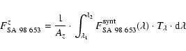 |
(A.4) |
 |
(A.5) |
 |
(A.6) |
 |
(A.7) |
| Fz A0V | = | ||
| = |
In order to transform the colours and magnitudes of the isochrones
reported by Baraffe et al. (1998) and Chabrier et al. (2000) into the WFI-Cousins system
we determined first the WFI synthetic magnitudes,
![]() ,
as
,
as
In order to compute the expected flux of a PMS star or a young BD in
the pass-band
![]() of a given filter we proceeded as follows.
We first determined the transmission curve,
of a given filter we proceeded as follows.
We first determined the transmission curve,
![]() ,
i.e. the product of the detector quantum efficiency and the given
filter transmission curve
,
i.e. the product of the detector quantum efficiency and the given
filter transmission curve![]() .
We then compute
.
We then compute
 |
(B.2) |
 |
(B.3) |
![\begin{figure}
\par\resizebox{8.8cm}{!}{\includegraphics[width=12cm,height=13cm]{6500figB1.ps}}
\end{figure}](/articles/aa/full/2007/28/aa6500-06/img202.gif) |
Figure B.1:
The R, I, z (upper panel),
|
![\begin{figure}
\par\includegraphics[width=7cm,height=9cm,clip]{6500figB2.ps}
\end{figure}](/articles/aa/full/2007/28/aa6500-06/img203.gif) |
Figure B.2: The Cousins colours as a function of the WFI instrumental colours for the standard stars in the Landolt's field SA 98. The continuous lines display the best fit of the data while the dashed lines have slope equal to 1 (i.e. no correction). |
As an example of our procedure we show in
Fig. B.1 (upper panel) two model spectra and the R,
I and z WFI+ESO2.2m transmission curves over-plotted. However,
the flux
![]() that we obtained in this way is the
one at the surface of the star. The observed flux at any distance
(d) is given by
that we obtained in this way is the
one at the surface of the star. The observed flux at any distance
(d) is given by
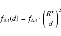 |
(B.4) |
Note that, consistently with the RIz photometric calibration of
the sources in Cha II, the absolute calibration constants used
in Eq. (B.1) are those of the WFI-Cousins photometric system
(see Table 5). However, a non-negligible difference
between the I-WFI and the I-Cousins pass-bands arises from the
fact that the red cut-off of the I-WFI filter is defined by the
CCD response and it is centred on a redder wavelength (0.85 ![]() m)
with respect to the standard Cousins I filter (0.79
m)
with respect to the standard Cousins I filter (0.79 ![]() m).
In order to take into account this difference in the determination
of the theoretical isochrones, we have exploited the relations
between the WFI-Cousins (R-I)C and (IC-z) standard colours
and the WFI instrumental colours for the standard stars in the
Landolt's fields.
By a least-square linear fitting (Fig. B.2), we derive the
coefficients which allow us to correct the colours of the computed
isochrones
m).
In order to take into account this difference in the determination
of the theoretical isochrones, we have exploited the relations
between the WFI-Cousins (R-I)C and (IC-z) standard colours
and the WFI instrumental colours for the standard stars in the
Landolt's fields.
By a least-square linear fitting (Fig. B.2), we derive the
coefficients which allow us to correct the colours of the computed
isochrones
 |
(B.5) |
 |
(B.6) |
In Fig. B.3, the 1, 5 and 10 Myr isochrones by Chabrier et al. (2000) are compared with those derived by us in the WFI-Cousins photometric system. Note the large difference, in particular for the coolest objects, i.e. (R-I)C >1.7, where the use of the isochrones in the Bessel-Cousins system would have produced many spurious member candidates.
In order to check our procedure, we used the standard filters of Bessel (1990) and we were successful in reproducing the isochrones presented by Chabrier et al. (2000) (see the smaller panel in Fig. B.3).
![\begin{figure}
\par\resizebox{8.8cm}{!}{\includegraphics[width=8.5cm,height=6.5cm]{6500figB3.ps}}
\end{figure}](/articles/aa/full/2007/28/aa6500-06/img208.gif) |
Figure B.3: Theoretical isochrones by Baraffe et al. (1998) and Chabrier et al. (2000) for the Cousins photometric system of Bessel (continuous line) and for the WFI-Cousins system (dashed lines, this work). In the smaller panel the 5 Myr isochrone by Chabrier et al. (2000) (continuous line) is compared with that reproduced by our algorithm when using the same Bessel filters (dashed line). |
These objects were selected as member candidates of Cha II
by Young et al. (2005) on the basis of MIPS@Spitzer observations.
IRAS F12488-7658/C 13 was also previously proposed as a young object by (Vuong et al. 2001).
We cannot conclude whether our selection criteria are satisfied
for these objects because they are saturated in at least one of the
three broad-bands RIz. However, their (
![]() )
indices suggest H
)
indices suggest H![]() emission (see Table 7) at
emission (see Table 7) at ![]() 2
2![]() level and their
location on the (J-H) vs. (H-K) diagram is consistent with
the PMS stars locus (see Sect. 4 and Fig. 10).
level and their
location on the (J-H) vs. (H-K) diagram is consistent with
the PMS stars locus (see Sect. 4 and Fig. 10).
ChaII 376 was the only H![]() emitter detected by López-Martí et al. (2005)
in their WFI pointing.
They also proposed that their candidates ChaII 304 and ChaII 305 are two
low-mass BDs or planetary-mass objects close to the Deuterium burning limit.
These two objects, however, do not satisfy our selection criteria.
The early classification of these objects as possible Cha II members
by López-Martí et al. (2005), though based on WFI images taken with the same set of
filters as in our survey, is probably not accurate
because the isochrones in the Cousins system of Bessel (Chabrier et al. 2000) used
for the selection are inadequate for the WFI-Cousins photometric system
(see Appendix B). From their dereddened (
m856-m914) colour
index we estimate an effective temperature of 2800 K and 3000 K for ChaII 304
and ChaII 305, respectively. Assuming these temperature values, we find
that the location of the two objects on the HR diagram would be
inconsistent with membership to Cha II.
We found that the optical colours of ChaII 376 are inconsistent
with membership, as also asserted by López-Martí et al. (2005), and we do not
detect any significant H
emitter detected by López-Martí et al. (2005)
in their WFI pointing.
They also proposed that their candidates ChaII 304 and ChaII 305 are two
low-mass BDs or planetary-mass objects close to the Deuterium burning limit.
These two objects, however, do not satisfy our selection criteria.
The early classification of these objects as possible Cha II members
by López-Martí et al. (2005), though based on WFI images taken with the same set of
filters as in our survey, is probably not accurate
because the isochrones in the Cousins system of Bessel (Chabrier et al. 2000) used
for the selection are inadequate for the WFI-Cousins photometric system
(see Appendix B). From their dereddened (
m856-m914) colour
index we estimate an effective temperature of 2800 K and 3000 K for ChaII 304
and ChaII 305, respectively. Assuming these temperature values, we find
that the location of the two objects on the HR diagram would be
inconsistent with membership to Cha II.
We found that the optical colours of ChaII 376 are inconsistent
with membership, as also asserted by López-Martí et al. (2005), and we do not
detect any significant H![]() emission for this object.
Moreover, its R-band magnitude (16.31 mag) is remarkably brighter
than the one reported by López-Martí et al. (2005) (18.38 mag). Since the
magnitude of this object in the other bands are in fair agreement
with ours, we think that the R-band magnitude reported in
López-Martí et al. (2005) may be incorrect. This may explain why ChaII 376
was selected as their only H
emission for this object.
Moreover, its R-band magnitude (16.31 mag) is remarkably brighter
than the one reported by López-Martí et al. (2005) (18.38 mag). Since the
magnitude of this object in the other bands are in fair agreement
with ours, we think that the R-band magnitude reported in
López-Martí et al. (2005) may be incorrect. This may explain why ChaII 376
was selected as their only H![]() emitter.
emitter.
This is one of the 19 PMS stars originally identified by Schwartz (1977)
in Cha II. Subsequent photometric observations by Hughes & Hartigan (1992) showed
that the object is a visual triple system. The H![]() emission
star originally discovered by Schwartz (1977), Sz 46N, has two companions,
namely Sz 46NW and Sz 46S; both are bluer than Sz 46N and are probably
unrelated to it (Hughes & Hartigan 1992).
Based on our analysis, both Sz 46NW and Sz 46S have optical colours
inconsistent with membership to the Cha II cloud, their temperature is
well above 4000 K according to their (
m856-m914) index and
the (
emission
star originally discovered by Schwartz (1977), Sz 46N, has two companions,
namely Sz 46NW and Sz 46S; both are bluer than Sz 46N and are probably
unrelated to it (Hughes & Hartigan 1992).
Based on our analysis, both Sz 46NW and Sz 46S have optical colours
inconsistent with membership to the Cha II cloud, their temperature is
well above 4000 K according to their (
m856-m914) index and
the (
![]() )
colour suggests no H
)
colour suggests no H![]() emission.
Thus, Sz 46NW and Sz 46S are most probably not PMS stars and hence, not
physically associated with Sz 46N.
emission.
Thus, Sz 46NW and Sz 46S are most probably not PMS stars and hence, not
physically associated with Sz 46N.
These objects were detected as ROSAT X-rays sources (Alcalá et al. 2000) and proposed as possible members of Cha II by different authors (Larson et al. 1998; Prusti et al. 1992; Young et al. 2005).
IRAS 12533-7632 appears on our images as a point-like object
associated with a nebulosity, consistently with what reported
in Prusti et al. (1992). However, it was not detected in our z and
H![]() images; its RI magnitudes and 2MASS near-IR colours
are inconsistent with those expected for a PMS star.
images; its RI magnitudes and 2MASS near-IR colours
are inconsistent with those expected for a PMS star.
In Young et al. (2005) IRAS F13052-7653 is reported as CHIIXR 60 which
is a non-existent identifier.
This must be a typo because IRAS F13052-7653 is identified with
the ROSAT source CHIIXR 37 (Alcalá et al. 2000).
The optical counterpart of IRAS F13052-7653 appears as a visual
triple system (Larson et al. 1998) whose components are designated as
IRAS F13052-7653N, IRAS F13052-7653NW and IRAS F13052-7653S in
Table 7.
None of the three components was recovered by our selection criteria,
most likely because their colours, both in optical and and near-IR,
may be contaminated. However, two of them, namely
IRAS F13052-7653N and IRAS F13052-7653NW, fall just below the
10 Myr isochrone and their (
![]() )
indices
suggest H
)
indices
suggest H![]() emission above 3
emission above 3![]() level (see Table 7); moreover,
their near-IR colours are also consistent with those expected
for PMS stars. IRAS F13052-7653S is not detected in 2MASS;
its optical colours are inconsistent with membership to Cha II and
its H
level (see Table 7); moreover,
their near-IR colours are also consistent with those expected
for PMS stars. IRAS F13052-7653S is not detected in 2MASS;
its optical colours are inconsistent with membership to Cha II and
its H![]() colour does not indicate significant emission.
colour does not indicate significant emission.
This object was detected in X-rays with ROSAT (Alcalá et al. 2000). Its optical and near IR colours are consistent with those of a PMS star with strong IR excess (see also Young et al. 2005). Previous authors (Allers et al. 2006; Vuong et al. 2001) report an extinction value significantly higher than the one determined by us (Table 6). Given the strong IR excess, our procedure for the temperature estimate provides unreliable results. Therefore, it may be a deeply embedded source or a highly reddened PMS star.
These sources were first detected by DENIS and
proposed as young stellar object candidates of Cha II
by Vuong et al. (2001) based on their IR colours and,
more recently, by Young et al. (2005) and Allers et al. (2006)
on the basis of IRAC@Spitzer and MIPS@Spitzer observations,
respectively. From the effective temperature and ![]() estimates provided in Table 6, and calculation of
their luminosities as explained in Sect. 5,
we estimate a mass of 0.08 and 0.06
estimates provided in Table 6, and calculation of
their luminosities as explained in Sect. 5,
we estimate a mass of 0.08 and 0.06 ![]() for C 62 and C 66, respectively. The age we derive
for both objects using the Baraffe et al. (1998) and Chabrier et al. (2000) tracks is
around 2 Myr. These estimates of mass and age are
fairly consistent with those derived by Allers et al. (2006).
From their H
for C 62 and C 66, respectively. The age we derive
for both objects using the Baraffe et al. (1998) and Chabrier et al. (2000) tracks is
around 2 Myr. These estimates of mass and age are
fairly consistent with those derived by Allers et al. (2006).
From their H![]() index we also notice strong line
emission (
index we also notice strong line
emission (![]() 3
3![]() level) in both objects (see Table 6).
level) in both objects (see Table 6).
This source has been detected in the near and mid-IR
by Persi et al. (2003), but it was first revealed as an X-ray
emitting source, CHIIXR3, by Alcalá et al. (2000).
The association of this object with IRAS 12551-7657 is
still unclear. Based on this evidence and
the effective temperature estimated by us (Table 6),
ISO-CHA II 29 is proposed to be a PMS star in Cha II
with a mass of about 1 ![]() .
.
None of these sources, originally identified by Persi et al. (2003),
was selected with MIPS@Spitzer by Young et al. (2005). These sources
do not satisfy our criteria and their (
![]() )
index suggests no emission in H
)
index suggests no emission in H![]() .
.
In our optical images, ISO-CHA II 98 appears as a visual binary,
but the colours and magnitudes of its components are inconsistent
with our selection criteria.
We stress that ISO-CHA II 98 was wrongly identified in
SIMBAD with the ROSAT X-ray source CHIIXR 24 by Alcalá et al. (2000).
The optical spectrum of CHIIXR 24 shows the Li I 6708 Å
absorption line, but the H![]() line is well in
absorption (Alcalá et al. 2000). Being classified as a G7-type star,
CHIIXR 24 is most likely a field object unrelated to Cha II.
line is well in
absorption (Alcalá et al. 2000). Being classified as a G7-type star,
CHIIXR 24 is most likely a field object unrelated to Cha II.
These sources are reported in the list of candidates by
Young et al. (2005). While 2MASS 13102531-7729085 and 2MASS 13110329-7653330
are rejected by our selection criteria, 2MASS 13125238-7739182
is selected as a PMS star candidate.
The first two sources have H![]() indices indicating no
H
indices indicating no
H![]() emission, while the H
emission, while the H![]() index of the last
suggests H
index of the last
suggests H![]() in emission at 1
in emission at 1![]() level. Thus, it is likely that
2MASS 13102531-7729085 and 2MASS 13110329-7653330 are
field stars unrelated to Cha II.
level. Thus, it is likely that
2MASS 13102531-7729085 and 2MASS 13110329-7653330 are
field stars unrelated to Cha II.
![\begin{figure}
\par\includegraphics[width=7cm,height=7cm]{6500fig7.ps}
\end{figure}](/articles/aa/full/2007/28/aa6500-06/img102.gif)