A&A 469, 949-961 (2007)
DOI: 10.1051/0004-6361:20066807

Effects of turbulent diffusion on the chemistry of diffuse clouds

P. Lesaffre - M. Gerin - P. Hennebelle

LERMA, CNRS UMR8112, Observatoire de Paris and ENS/LRA, 24 rue Lhomond, 75231 Paris Cedex 05, France

Received 24 November 2006 / Accepted 19 April 2007

Abstract
Aims. We probe the effect of turbulent diffusion on the chemistry at the interface between a cold neutral medium (CNM) cloudlet and the warm neutral medium (WNM).
Methods. We perform moving grid, multifluid, 1D, hydrodynamical simulations with chemistry including thermal and chemical diffusion. The diffusion coefficients are enhanced to account for turbulent diffusion. We post-process the steady-states of our simulations with a crude model of radiative transfer to compute line profiles.
Results. Turbulent diffusion spreads out the transition region between the CNM and the WNM. We find that the CNM slightly expands and heats up: its CH and H₂ content decreases due to the lower density. The change of physical conditions and diffusive transport increase the H⁺ content in the CNM which results in increased OH and H₂O. Diffusion transports some CO out of the CNM. It also brings H₂ into contact with the warm gas with enhanced production of CH⁺, H₃⁺, OH and H₂O at the interface. O lines are sensitive to the spread of the thermal profile in the intermediate region between the CNM and the WNM. Enhanced molecular content at the interface of the cloud broadens the molecular line profiles and helps exciting transitions of intermediate energy. The relative molecular yields are found higher for bigger clouds.
Conclusions. Turbulent diffusion can be the source of additional molecular production and should be included in chemical models of the interstellar medium (ISM). It also is a good candidate for the interpretation of observational problems such as warm H₂, CH⁺ formation and presence of H₃⁺.

Key words: astrochemistry - turbulence - diffusion - ISM: clouds - ISM: molecules - ISM: lines and bands

1 Introduction

In the thermally bistable neutral ISM, small structures of cold neutral gas (CNM for cold neutral medium, $T \approx 70$ K and $n \approx 50$ cm^-3) are immersed in the warm neutral medium (WNM, $T\approx 8000$ K and $n \approx 0.4$ cm^-3). Both phases are found to have approximately the same pressure (Heiles & Troland 2003). In this paper, we investigate how turbulent diffusion processes can affect the chemistry and the structure of an interface between a CNM cloudlet and the WNM.

Much of the knowledge on the cold diffuse medium has been established from the detection of molecules, radicals and molecular ions. Despite its relatively low density the diffuse interstellar medium is chemically active and furthermore, its chemistry is not fully understood (Snow & McCall 2006, and references therein). The presence of the reactive ions CH⁺ and H₃⁺ together with radicals like CH and C₂ and molecules like CO in the diffuse ISM can not be understood with steady state chemical models. For example, Le Petit et al. (2004) present a detailed modeling of the ISM along the line of sight of $\zeta$ Per which requires three components along the line of sight: a long (4 pc) diffuse region at 60 K, a tiny (100 AU) dense region at 20 K, both with a large ionization rate, and a series of shocks which account for the abundance of CH⁺ and the excited rotational populations of H₂. This example is not unique and demonstrates the necessity of coupling self-consistent models of the structure of the ISM with the chemistry. It also shows that CH⁺and H₃⁺ are key species for understanding the coupling of turbulence, dynamics and chemistry in the diffuse ISM.

The ubiquitous presence of CH⁺ and excited rotational lines of H₂, which are not expected at thermal equilibrium given the average temperatures of the cold neutral medium, indicates that non equilibrium processes must also be taken into account, which will bring enough energy locally to trigger the formation of CH⁺ and could contribute to the excitation of H₂. H₃⁺ is mainly formed with H₂ and H₂⁺ (itself resulting from the ionisation of H₂by a cosmic ray) and efficiently destroyed by dissociative recombination with electrons. As reviewed by Snow & McCall (2006), diffuse cloud models do not predict H₃⁺ to be abundant, except when the ionisation rate is high enough to maintain a large formation rate. Steady state chemistry predicts that the H₃⁺ density scales as: $n({\rm H}_3^+)= \frac{\zeta n({\rm H}_2)} {k_{\rm e} n\rm (e)}$. Because the H₃⁺ density is approximately constant and proportional to $\zeta$, the presence of large H₃⁺ column densities requires long pathlengths through the CNM (4 pc for $\zeta$ Per as modelled by Le Petit et al. 2004, and using $\zeta = 25 \times 10^{-17} ~\rm s^{-1}$) which significantly exceed the expected size of such structures (e.g. around 0.1 pc up to 1 pc in the simulations by Audit & Hennebelle 2005). The problem with the path length is even more severe because the determined column density of H₃⁺ towards $\zeta$ Per requires a path length larger than 60 pc when using the standard value for the cosmic ray ionisation rate, $\zeta \sim 3 \times 10^{-17} ~\rm s^{-1}$! As CNM cloudlets are never isolated but always immersed in the WNM, we investigate in this paper the effect of turbulent diffusion at their interface as an alternative solution for enhancing molecular abundances in the ISM. A subsequent paper will present the effects of shocks.

The chemical importance of turbulent diffusion has been acknowledged in the context of protostellar cores since the work of Boland & de Jong (1982) who realised how extra mixing could limit element depletion on grains. Since then, many authors have computed the effect of turbulent mixing on the chemistry of protostellar and prestellar cores. Chièze & Pineau des Forêts (1989) and Chièze et al. (1991) have used a simple two-zone model and a mixing prescription between the envelope and the cores of these objects. Xie et al. (1994) and Xie et al. (1995) computed the isothermal evolution of chemistry with an enhanced diffusion coefficient. Willacy et al. (2002) later extended this work including H₂ photo-dissociation and gas-grain interactions. Rawlings & Hartquist (1997) did similar computations but using a uniform pressure and a diffusion term based on numerical densities rather than a Fick law based on mass fraction.

In the present study, we transpose this series of work to another context with physical conditions at lower densities and lower visual extinctions, more appropriate to the diffuse neutral ISM. We also improve on the previously used numerical methods. First, we compute the hydrodynamical evolution of a multifluid gas and we treat the gas cooling in a self-consistent manner, completely coupled to the chemical evolution. Second, we model the turbulent diffusion of temperature along with chemical mixing: this will prove useful to extend the region where the formation of molecules is favoured.

In Sect. 2 we describe our numerical method. We present our results in Sect. 3 and discuss them in Sect. 4. Section 5 draws our conclusions.

2 Method

We use the multifluid monodimensional (plane parallel) magnetohydrodynamical (MHD) code presented in Lesaffre et al. (2004). This code fully couples the hydrodynamics and the chemistry. It also makes use of a moving grid algorithm (Dorfi & Drury 1987) which allows to spatially resolve the shock discontinuities and the diffusion fronts. In order to model the diffuse molecular gas we had to supplement the code with the following new processes.

2.1 Radiative transfer

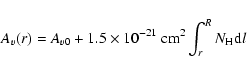
A radiation field equal to the standard interstellar radiation field (ISRF) illuminates the right hand (outer) side of the computational box. The extinction at the outer side of the box is very small: A_v0=0.01, relevant to WNM conditions. The extinction at any point inside the computational box is given by

$$A_v(r)=A_{v0}+1.5 \times 10^{-21}~{\rm cm}^2 \int_r^R N_{\rm H} {\rm d}l$$ (1)

where r is the position inside the computational box, R is the position at the outer (right hand) edge of the box and $N_{\rm H}$ is the numerical density of hydrogen nuclei (hence A_v actually increases from right to left). In most simulations of this paper, the total A_v(0) across the box is 0.14 mag for a total length of the box R=5 pc: we refer to them as "Small cloud'' (or standard) simulations. In some other simulations, we used A_v(0)=1.4 mag and R=10 pc ("Big cloud'' simulations). The local value of A_v is used to determine the heating rate due to the photo-electric effect on grains and various photo-chemical rates (see below).

The dense cloud will therefore naturally be formed at the left hand side of the computational box, where the extinction is the highest. The WNM will be found at the right hand side.

2.2 Photo-chemistry

The reaction network in Lesaffre et al. (2004) has been extended with photo-chemical reactions of dissociation and ionisation. The total number of reactions is now 138. The full list of reactions can be found in the last appendix of Lesaffre (2002) and takes its main roots in the early work of Chièze et al. (1998): it is designed to account for the abundances of the main cooling agents of the ISM such as C⁺, C, O, H₂, OH, CO and H₂O. The dependence of each photo-reaction rate on the local radiation field is modeled with a parameter $\beta$. The local rate is obtained by multiplying the rate for the ISRF by the factor $\exp~(-\beta A_v)$. In most cases, this simple rule is sufficient to get an accurate model for the extinction of the radiation field in the wavelength range relevant to a given photo-reaction.

However, the photo-dissociation of the molecule H₂ requires a special treatment because of its self-shielding properties. For this purpose, we use Eq. (37) of Draine & Bertoldi (1996) with a constant Doppler parameter of b₅=0.1 corresponding to a 0.1 km s^-1 Doppler broadening (this small value maximises the effect of self-shielding). Note that due to the small total column-density across our computational box, we do not need a similar treatment for the photo-dissociation of CO.

In the present simulations we use $1.5\times 10^{-7}$ cm^-3 s^-1 at 300 K for the dissociative recombination rate of H₃⁺ with a cosmic ray ionisation rate of $\zeta=5\times 10^{-17}$ s^-1.

2.3 Diffusion

The structure and evolution of a front between a CNM cloudlet surrounded by the WNM are mainly determined by diffusion processes. Diffusion is due to random motions which transport thermal energy or chemical species. It can be caused either by microscopic collisions between molecules or by random macroscopic motions of turbulent eddies.

In the following, we evaluate diffusion coefficients for these two modes of diffusion.

   
2.3.1 Molecular diffusion

It is a difficult task, still heavily discussed, to determine the diffusion coefficients in a multi-component plasma. Here, we adopt a simple view consistent with our modeling of three different fluids: neutrals, ions and electrons.

A typical molecular flight takes place at the thermal velocity over a length scale equal to the mean free path. We hence adopt diffusion coefficients of the form

$$d_j=c_j \lambda$$ (2)

with j = n, i, e spanning the neutral, ion and electron fluids, where $\lambda=1/\sigma N$ is the mean free path ( $\sigma=10^{-15}$ cm² and N is the total number density of particles per cm³) and

$$c_j=\sqrt{\frac{5 {k} T_j}{3 \mu_j}}$$ (3)

is the sound speed in fluid j (k is the Boltzmann constant, T_j is the temperature of fluid j and $\mu_j$ its average molecular weight). We assume that electrons are dynamically coupled to the ions and hence take $d_{\rm e}:=d_{\rm i}$. According to the relative average molecular weights, diffusion is fastest in the neutral fluid and slowest in the ion and electron fluid. It is a bit artificial to adopt the same mean-free path for all three components independent of energy, but as long as these length scales are much smaller than the turbulent diffusion lengths scales, our results should not be changed.

The thermal diffusion term takes the form

$$\frac{\partial }{\partial r}\left(\widetilde{N_jd_j}\frac{\partial {k} T_j}{\partial r}\right)$$ (4)

in the evolution equation for the energy density for each fluid j. N_j is the number density of particles in fluid j. $\widetilde{N_jd_j}$ is N_jd_j interpolated linearly at each interface of the computational zones and diffusion fluxes are assumed to vanish at the computational boundaries.

We adopt a similar treatment for the chemical diffusion term

$$\frac{\partial }{\partial r}\left(\widetilde{\rho d_j}\frac{\partial X_i}{\partial r}\right)$$ (5)

in the evolution equation for the number density N_i of species iin fluid j, with X_i the mass fraction of species i and $\rho$the total mass density. Note that we do not take into account the individual thermal velocities for each species but we rather take the average sound speed in each corresponding fluid. This may be improved in future work.

2.3.2 Turbulent diffusion

Consider the evolution equation of the number density N of a given chemical species (of mass fraction X) with velocity $\vec{U}$, net chemical production rate R and diffusion coefficient d:

$$\frac{\partial N}{\partial t}+{\bf\nabla.}(N\vec{U})=R+ {\bf\nabla.}[d\rho{\bf\nabla} X] \mbox{.}$$ (6)

Our purpose is to find an evolution equation for the quantity N averaged over a given length scale l, which we denote $\overline{N}$. The average of Eq. (6) yields

$$\frac{\partial \overline{N}}{\partial t}+{\bf\nabla.}(\overl... ...rline{d\rho{\bf\nabla} X}] -{\bf\nabla.}\overline{(n \vec{u})}$$ (7)

where $\vec{u}=\vec{U}-\overline{\vec{U}}$ and $n=N-\overline{N}$.

The challenge of turbulent models resides in the difficulty of finding a simple but accurate model for the behaviour of high order moments such as ${\bf\nabla.}\overline{(n \vec{u})}$. We now sketch a brief justification for the crude model we adopted. We compute the time evolution of n under the first order smoothing approximation (FOSA) which allows us to drop all orders higher than two. The difference between Eqs. (6) and (7) yields

$$\frac{\partial n}{\partial t}+{\bf\nabla.}(n\vec{U})= -{\bf\nabla.}(\overline{N}\vec{u})+(R-\overline{R})$$ (8)

where we neglected second order terms and safely dropped the term proportional to d since it is generally small compared to the turbulent diffusion. The term $R-\overline{R}$ arises because of differential reactivity in turbulent eddies (see Lesaffre et al. 2005) and can be neglected provided the turbulent mixing time scales are much shorter than the chemical time scales. That is hard to justify, and can in fact be wrong for most of the rapidly reacting species, but we will neglect this term in the present work for the sake of simplicity. Note that we also make the convenient approximation $\overline{R(N)}=R(\overline{N})$ which is consistent with our neglect of differential reactivity.

We now assume that n is given by the integration of the source term in Eq. (8) over a given correlation time $\tau$, sufficiently short to neglect the time evolution of spatially averaged values. This leads us to the expression for the turbulent term in Eq. (7):

$$-{\bf\nabla.}\overline{(n\vec{u})}={\bf\nabla.}[\overline{ \tau{\bf\nabla.}(\overline{N}\vec{u})\vec{u}}] \mbox{.}$$ (9)

Mass conservation of the averaged quantities requires $\overline{N}=\overline{\rho}~\overline{X}$. We use this relation to expand the previous relation:

$$-{\bf\nabla.}\overline{(n\vec{u})}= {\bf\nabla.}[\overline{\r... ... {\vec{u} \otimes \nabla}){\bf .} (\overline{\rho}~\vec{u})}].$$ (10)

We retain only the first term which is analogous to a diffusion term with a tensor turbulent diffusion coefficient $K=\overline{ \tau \vec{u} \otimes \vec{u}}$ which simplifies to a scalar $K=\frac13\overline{\tau u^2}$ for isotropic turbulence. The second term is an advection term that is present only when turbulence carries a non zero net mass flux.

Under these simplifying assumptions, the effect of an underlying turbulent velocity field can hence be reduced to an effective diffusion coefficient K. A good discussion of the observational uncertainties on K can be found in Xie et al. (1995). In brief, we have a good idea of the rms fluctuations of the velocity field from the broadening of spectral lines, but we only have a poor understanding of the correlation length scale (or equivalently of the correlation time scale) of the turbulence.

Given these uncertainties, we investigated several possibilities for the value of K. For all computations with turbulent diffusion presented in this paper, we keep the same formulation as for the molecular diffusion coefficients d_j above, but we use a fixed correlation length L instead of $\lambda$ and the sound speed $c_{\rm n}$in the neutrals for all fluids. This implicitly assumes that the turbulent diffusion coefficient scales as the local average sound speed, which may be questionable. On the other hand, it yields smaller diffusion coefficients in colder parts of the cloud and it implies that the ratio of the thermal pressure to the turbulent pressure is a fixed constant, which seems reasonable (in particular, it gives a uniform turbulent pressure field when the thermal pressure itself is uniform). We also tested the more simple uniform prescription $K=L\times 0.2$ km s^-1 (similar to Xie et al. 1995) but we did not find any significant qualitative difference with the results presented here. In all our tests, we adopted the same diffusion coefficient for the chemistry and the temperature.

3 Results

3.1 Numerical setup

In this section, we investigate the steady state of condensation fronts by means of time-dependent simulations evolved over very long times. We prepare a cold state (CNM) and a hot state (WNM) of thermochemical equilibrium at a given total pressure $P_0=3\times 10^{3}$ K cm^-3 for a given extinction A_v0=0.01. More precisely, we evolve a two-zone isobaric model until both zones achieve a steady state of thermal and chemical equilibrium at A_v0=0.01, hence the initial molecular content is small. Our adopted values for the abundance of C and O gas phase are $1.3\times 10^{-4}$ and $4.3\times 10^{-4}$ respectively. We then select a length l (l=0.5 pc in for our small cloud simulations and l=5 pc for our big cloud simulations) for the cold "cloud'' which will be located to the left (inner) side of the computational box and the rest of the box (of total length R=5 pc or 10 pc in the small or big cloud simulations) is filled with the hot state. We then let the gas evolve chemically and hydrodynamically in the box. This procedure essentially sets only the total mass in the box, as the size of the cloud and the pressure will later relax according to the hydrodynamical, thermal and chemical evolution. We later refer to the small cloud simulation without turbulent diffusion as our reference run.

	Figure 1: Reference run (small cloud without turbulent diffusion): time evolution of H2 (solid, value scaled by a factor 10-6), CO (solid), OH (dotted), H2O (dashed), H3+ (dash-dotted), CH+ (dash-dot-dot-dot) and CH (long-dash) column-densities (cm-2) integrated over the computational box.
Open with DEXTER

3.2 Evolution of the small cloud without turbulent diffusion (reference run)

The chemistry first reacts to the new local A_v>A_v0, with molecules reforming in the cloud. Another transient effect is due to the partial pressure of ions and electrons which differ in the cold and hot phase due to fractional abundance differences. The gradient of partial pressures generates a flow of ions across the surface of the cloud. This process is responsible for a transient chemistry which we do not describe here, as it mainly results from our arbitrary initial conditions. Microscopic (molecular) thermal and chemical diffusion then build up a smooth spatial transition between the cold and hot phases.

We give the time evolution of the total column densities of several species in Fig. 1 as an illustration of the very long times required to reach a steady state. One after the other, chemical reactions reach their steady state according to their own time scales. After a time of about 0.1 Gyr chemical equilibrium is achieved and the shape of the diffusion front (Fig. 3) reaches an approximate steady-state. However, it is not stationary yet as it is moving from the hot towards the cold medium, with the cold medium reaching colder temperatures and higher molecular fractions. The cloud shrinks in size as the condensation front moves and its density gets higher while the hot medium gets hotter and more diffuse. Note that the overall pressure rises while the front tries to adjust the total cooling rate to the total heating rate, on its way to find a steady state.

This simulation did not show any sign of reaching a steady state after more than 1 Gyr. However, extrapolating the 0.1 Gyr time scale to reach steady state in our lowest turbulent diffusion coefficient to 20 times lower diffusion would give a time scale of 2 Gyr. This computation may hence not have been carried out over a long enough time to probe if this front will eventually reach a steady state or not.

The multifluid nature of our computations is not essential to the present study. Nevertheless, it allows us to uncover a potentially interesting partial pressure effect. A slight neutral/charges velocity drift of the order of 0.01 km s^-1 persists in the hot phase throughout the simulation. This drift is sustained by the partial pressure equilibration. Indeed, photo-ionisation is more effective in the hot phase and a partial pressure gradient drives a flow of charged ions towards the cold medium. This is the cause of a current of charges from the hot toward the cold medium: C⁺ ions accumulate at the surface of the cloud where their radiative cooling produces a dip in the temperature profile (see Fig. 3). If self-gravity of the cloud was taken into account, this would produce a convective instability at the surface of the cloud that would soon smooth out the temperature and C⁺ profiles. This C⁺ effect might also be responsible for the failure of the front to reach a completely static state.

3.3 Effect of turbulent diffusion

Although we display the results for big cloud simulations, we restrict our analysis to small cloud simulations in this section. The big cloud simulation was run following the same numerical experiment as for the small cloud, but we investigated only two different values for the turbulent diffusion coefficient. Big cloud simulations are discussed in Sect. 4.1.

We restart our computation from t=0.1 Gyr in the reference run and switch on turbulent diffusion while resetting the time to 0. After about another 0.1 Gyr has occurred, a static state is reached. The time to reach a steady state is much shorter than in the case without diffusion, because the effective diffusion time scales are much smaller. The ion current is still present, but the diffusion smoothes out the dip in temperature and in C⁺composition. This seems to allow the front to find a final equilibrium. The pressure in this final equilibrium turns out to be nearly 40% less than in the case without turbulent diffusion at time 0.1 Gyr.

We now probe the dependence of this steady state on the magnitude of the turbulent diffusion coefficient. We compare the state of the simulation box at time 0.1 Gyr for different turbulent length scales L ranging from $1.25\times 10^{-4}R$ to $1.6\times 10^{-2}R$ with a factor 2 increment. With R=5 pc, this range extends from $L=6 \times 10^{-4}$ pc to L=0.08 pc. Note that the mean free path is at a scale of around $3 \times 10^{-5}$ pc in the cold medium, which corresponds to $6 \times 10^{-6} R$ and makes molecular diffusion negligible by at least a factor 20 with respect to turbulent diffusion in all our computations. The upper bound L=0.08 pc is roughly a seventh of the size of the cold cloud at this level of diffusion (remember L is set as a fraction of the size of the computational box but it is difficult to predict what the actual size of the cloud will be before actually running the simulation). As a point of comparison, Xie et al. (1995) built their diffusion coefficients with L=0.1-0.5 pc and a fixed velocity of 1 km s^-1 for a molecular cloud of size 1 pc.

Figure 2: CO (solid), OH (dotted), H2O (dashed), H3+(dash-dotted), CH+ (dash-dot-dot-dot) and CH (long-dash) column-densities (cm-2) integrated over the computational box for condensation fronts at time 0.1 Gyr with various diffusion lengths L(the big cloud run with the highest L is actually displayed at time 0.02 Gyr, when the WNM has disappeared). Plus signs are for the small cloud and diamonds stand for the big cloud runs. Note that the values for the runs without turbulent diffusion at time 0.1 Gyr have been arbitrarily placed at $L=3 \times 10^{-5}$ pc (small cloud) and L=0.1 pc (big cloud).

Open with DEXTER

Figure 2 displays the total column-densities of the molecular species of main interest for various diffusion coefficients. Except for the column-densities of CH which decreases, and those of CO and H₃⁺ which stay at the same level, the effect of turbulent diffusion is to boost the production of molecular species. In the following, we proceed to a more detailed investigation of the structure of the front: for each molecule of interest in each simulation, we computed which source and sink terms were dominant, including reaction and diffusion effects. This reveals that H₂molecules mixed into hot gas are the main cause for the diffusion-enhanced production of molecules.

3.3.1 Thermal and density structure

As illustrated in Fig. 3, the main effect of increasing the diffusion is to spread out the length of the front. As a result of the heat exchange between the hot and the cold phase, the cold phase becomes slightly hotter and the hot phase becomes slightly colder.

As already mentioned, the total pressure at steady state decreases when diffusion is enhanced. Besides, the cold medium temperature increases slighlty in the case with diffusion. As a result, the total density in the cloud decreases by more than a factor 2 in the case with diffusion (see Fig. 4). The cloud expands to keep its total column-density constant (remember that the total mass of the simulation box remains constant).

Everywhere in all simulations the dominant heating process is the photo-electric effect. The main cooling processes are from the inside of the cloud to the WNM (left to right): C⁺ cooling, diffusive cooling (on the WNM side of the diffusion front) and H (Lyman $\alpha$) cooling. In the WNM, O cooling is also important, but amounts to at most a half of the Lyman $\alpha$ cooling. When turbulent diffusion is present, molecules are abundant in the WNM (see below) and H₂ cooling sets in in between the region where diffusive cooling and Lyman $\alpha$ cooling prevail. Note that although O collisional excitation by electrons is adopted, we use H₂ cooling functions from Le Bourlot et al. (1999) which include excitation by H, He and H₂ only.

Figure 3: Temperature (K) structure of the front at steady-state for various diffusion coefficients: a) upper panel (standard run) the solid line is for molecular diffusion, the dotted line for $L=6 \times 10^{-4}$ pc, the dashed line for L=10-2 pc and the dash-dotted line for $L=8 \times 10^{-2}$ pc; b) lower panel (big cloud run) the solid line is for molecular diffusion, the dotted line for L=0.16 pc and the dashed line for L=0.8 pc.

Open with DEXTER

	Figure 4: Density (cm-3) structure of the front for various diffusion coefficients (same labels as Fig. 3).
Open with DEXTER

3.3.2 H₂ abundance

The abundance of H₂ usually results from the balance between its formation on grains and its destruction by photodissociation. However, for cases with turbulent diffusion, in the intermediate region between the CNM and the WNM, the main source of H₂ is the divergence of its diffusive flux.

An increase in the diffusion coefficient considerably enhances the abundance of H₂ in the diffusion front (see Fig. 5). This is mainly a diffusion effect: diffusion mixes the cold molecular gas from the cloud with the external hot atomic gas. The diffusion flux provides a source of H₂ molecules in the hot phase which is strong enough to counteract photo-dissociation and manages to sustain high concentration levels of H₂ in a hot medium. Hence turbulence brings H₂ molecules in contact with hotter gas: this effect will be the source of a lot of efficient molecular chemistry.

The decrease in H₂ abundance in the cloud for enhanced diffusion results from the combined effects of the general spread in H₂(diffusion pumps H₂ from the cold cloud) and the lower density (H₂ formation on grains is less efficient).

	Figure 5: Abundance profile of H2 for various diffusion coefficients (same labels as Fig. 3).
Open with DEXTER

3.3.3 CH⁺ abundance

The most spectacular consequence of increasing the temperature of H₂ rich gas is the production of the CH⁺ molecular ion. In absence of diffusion, CH⁺ is produced via the reaction C⁺ + H  $\rightarrow$ CH⁺ and destroyed by photodissociation in the hot gas or by CH⁺ + H  $\rightarrow$ C⁺ + H₂ in the cold gas.

However, the reaction C⁺ + H₂  $\rightarrow$ CH⁺ + H can be a much more efficient source for CH⁺ provided that the 4640 K activation temperature is overcome in presence of H₂. As clearly seen in Fig. 6, diffusion provides an excellent means of bringing together high temperature and H₂ rich gas in order to make CH⁺ through this channel.

	Figure 6: Abundance profile of CH+ for various diffusion coefficients (same labels as Fig. 3).
Open with DEXTER

3.3.4 H₃⁺ abundance

H₃⁺ is made via the reaction H₂⁺ + H₂  $\rightarrow$ H₃⁺ + H and destroyed through dissociative recombination with electrons. As a result, n(H $_3^+)= {\zeta n({\rm H}_2)}/ {k_{\rm e} n\rm (e)}$ remains valid throughout most of the region where H₃⁺ is present. The recombination rate $k_{\rm e}$ is a decreasing power of the temperature (it behaves like $1/\!\sqrt{T}$). Furthermore, it turns out that the electron abundance $n\rm (e)$ also scales approximately like $\sqrt{T}$ in the intermediate region. One should therefore expect more H₃⁺ in the hot phase. However, photo-dissociation usually destroys the source of H₂ molecules in the hot phase. Turbulent diffusion allows to replenish part of the high temperature gas in H₂ molecules. This effect produces a peak of H₃⁺ inside the diffusion front as illustrated in Fig. 7.

	Figure 7: Abundance profile of H3+ for various diffusion coefficients (same labels as Fig. 3).
Open with DEXTER

3.3.5 OH abundance

In our simulations, OH usually results from the competition between the recombination of H₂O⁺ and photo-dissociation (for the conditions where the H₂ fraction is greater than about 0.2-0.3, H₂O⁺ is destroyed by H₂ and recombination of H₃O⁺becomes the main source, Pineau des Forêts 2007, private communication). However, the H-atom transfer O + H₂  $\rightarrow$ OH + H can become the dominant source if its 2980 K activation temperature is overcome in presence of H₂. Figure 8 shows that this is indeed the case at the CNM/WNM interface when turbulent diffusion is able to bring enough H₂ at sufficiently high temperature.

An other noticeable effect of turbulent diffusion is a factor 3 to 5 rise of the relative abundance of OH in the cold cloud from the case without turbulent diffusion to the case with turbulent diffusion. This is less straightforward to understand. Indeed diffusion slightly increases the temperature and strongly decreases the density in the cold cloud which is expected to decrease the recombination rate of H₂O⁺, hence lowering the OH abundance. However, H₂O⁺comes from H⁺ via the reaction H⁺ + O  $\rightarrow$ O⁺ + H followed by OH⁺ + H₂  $\rightarrow$ H₂O⁺ + H. The former reaction is subject to a 227 K activation temperature, which rate increases by at least a factor 6 in the cold cloud between the case with and without diffusion. H⁺ is itself subject to at least a factor 3 rise in relative abundance in the cold medium due to its lower recombination rate thanks to a slightly higher temperature and a less dense gas (the electron fraction remains roughly the same, as it is bound to the abundance of C⁺). The net effect is a rise in OH relative abundance due to the change in the physical conditions inside the CNM.

The very sharp dip in OH relative abundance at the surface of the cloud when turbulent diffusion is switched off (see the solid line in Fig. 8) is in fact composed of two dips. The inner one is caused by the dip in temperature and the sensitivity of the H⁺ + O reaction rate to temperature. The outer one is caused by the decrease of H₂that lowers the H₂O⁺ rate of production in a region where O + H₂ is not activated yet. Only the outer dip remains for $L=6~\times~10^{-4}$ pc (see the dotted line in Fig. 8).

	Figure 8: Abundance profile of OH for various diffusion coefficients (same labels as Fig. 3).
Open with DEXTER

3.3.6 CO abundance

In the densest parts of the cloud, CO is produced through the reaction HCO⁺ + e^-  $\rightarrow$ CO + H. That reaction accounts for the inner 0.1 pc in the small cloud cases and the inner 3 pc for the big cloud with the highest turbulent diffusion coefficient (in the latter case, CH +O  $\rightarrow$ CO + H also prevails in the inner 0.5 pc). HCO⁺ is indeed pointed out as one of the most likely sources for CO in diffuse and translucent clouds (Liszt & Lucas 1998).

In the rest of the simulation box, the molecule CO is most often produced by C⁺ + OH  $\rightarrow$ CO + H⁺ and destroyed by photo-dissociation. In these regions its relative abundance is hence directly linked to the relative abundance of OH and density, as demonstrated by Fig. 9. In a small region at the right hand side of the diffusion front, the reaction CO⁺ + H  $\rightarrow$ CO + H⁺ is the most efficient source of CO. For high diffusion coefficients, the abundance profile of CO can also be subject to diffusive mixing that removes CO from the CNM. The enhanced CO in the front, due to enhanced OH, is never strong enough to produce a significant local maximum in the diffusion front.

	Figure 9: Abundance profile of CO for various diffusion coefficients (same labels as Fig. 3).
Open with DEXTER

3.3.7 H₂O abundance

H₂O is generally produced by the recombination of the molecular ion H₃O⁺, which comes from proton exchange between H₂O⁺ and H₂ and is hence linked to the abundance of H⁺ as is OH in the cold cloud. H₂O experiences the same rise in abundance as OH in the cold cloud (see Fig. 10) but has an extra dependence on the H₂ fraction. This effect might be responsible for the actual decrease of the H₂O relative abundance in the CNM at high diffusion coefficients. However, the dominant source of H₂O in the diffusion front is proton exchange between H₂ and OH, as both molecules are abundant in the front for the reasons stated above.

	Figure 10: Abundance profile of H2O for various diffusion coefficients (same labels as Fig. 3).
Open with DEXTER

3.3.8 CH abundance

CH results from the dissociative recombination of CH₃⁺ and is mainly destroyed by photo-dissociation. CH₃⁺ is the result of two successive proton exchanges with H₂ starting from CH⁺.

The decrease of CH in the cloud is related to the decrease of the H₂ abundance (see Figs. 5 and 11). In the diffusion front, the enhanced CH⁺ abundance does not compensate for the higher temperature (which lowers the recombination rate) and the lower abundance of H₂.

The activation temperature of $1.41\times 10^4$ K for the reaction C + H $_2~\rightarrow~$CH + H is too high to be overcome in the same way as for CH⁺. Hence there is a net decrease of CH column-density when the diffusion is enhanced (the decrease comes from the lower H₂ abundance in the cloud).

	Figure 11: Abundance profile of CH for various diffusion coefficients (same labels as Fig. 3).
Open with DEXTER

3.3.9 Line profiles

We post-processed our simulations using a crude radiative transfer code in order to probe the effect of diffusion on the line profiles. We assume that a given species in each parcel of gas in the simulation emits (or absorbs) light with a Gaussian line shape in velocity space. The mean of the Gaussian is set to the local speed of the fluid, its width is set to the thermal speed of the species and its amplitude is set according to the column density of the parcel. Note that we implicitly assumed that the turbulent velocity is a constant fraction of the local sound speed. In this simple picture such turbulent motions do not modify the shape of the spectra if the velocity scale is expanded appropriately. We hence neglect the turbulent Dopper shifts and concentrate only on the intrinsic line shapes which reflect thermal and chemical changes.

In a first step, we don't take into account excitation effects. Assuming an optically thin medium, or a line profile seen in absorption, we compute the line shape across the box as the total column-density of species M per unit velocity bin centred on velocity v:

$$N_v(M,v)=\int_{0}^{R}{\rm d}r~ N(M)\exp{\left[-~\frac{\mu(u-v)^2}{2 {k} T}\right]} \sqrt{\frac{\mu}{2 \pi {k} T}}$$ (11)

where N(M) is the number density of species M, $\mu$ is its molecular weight, u is the local velocity of the fluid associated to M and T its temperature. Note that the integral of N_v(M,v) from $v=-\infty$ to $v=+\infty$ yields the total column-density of species M across the simulation box. Taking turbulence into account could be done simply by artificially decreasing $\mu$.

Figures 12 and 13 display N_v for a few molecules and atoms in the case without turbulent diffusion and in a case with turbulent diffusion. Without turbulent diffusion, all molecules show a narrow Gaussian profile corresponding to the temperature of the CNM. Indeed, molecules are absent from the WNM. C⁺ and O on the contrary are equally abundant in both phases and they show a wider secondary Gaussian feature, corresponding to emission from the WNM. The amplitude of this second Gaussian is smaller because there is much less total column-density in the WNM than in the CNM.

Figure 12: Line profile for H2O, CH+, CO and CH (see text). The solid line is in the case without turbulent diffusion, the dashed line is in the case with turbulent diffusion ( $L=8~\times~10^{-2}$ pc). A Gaussian line has been adjusted on the core of each profile (for velocities lower then 0.2 km s-1). It is displayed as a dotted line for the case without diffusion and as a dash-dotted line for the case with diffusion. In most cases, the dotted line cannot be distinguished from the solid line.

Open with DEXTER

When turbulent diffusion is present, molecules are formed in the transition layer at intermediate temperatures between the CNM and the WNM. This enhances the contribution of warm gas in the integral and gives rise to broad line wings. The effect is strongest in the case of CH⁺ which has the most efficient yield due to turbulent diffusion. The effect is inexistent for CH which subsists in the cold phase only. This provides a potentially powerful comparative probe between CH⁺ and CH. Indeed, CH⁺ lines are broader than CH and CO lines in the diffuse ISM (Pan et al. 2004).

We now compute the emission profiles of a few atomic transitions for which our code provides the level populations at steady-state (they are used to compute the atomic cooling functions). We integrate Eq. (11) using the local emissivities of these transitions instead of the quantity N(M). The results are displayed in Fig. 14. The fine-structure transitions of O show a strong effect with nearly exponential wings appearing in the case with turbulent diffusion. O has a nearly constant abundance across the simulation box. The wing effect in this case is entirely due to the structure in density and temperature. The fine structure transitions have energy temperatures of 227 K, 98 K and 326 K intermediate between the CNM and WNM temperatures. Besides, the critical density for O is much larger than the CNM density. It turns out that the emissivity of these O lines is highest in the intermediate temperature and density region inside the front. The change of integrated emissivity in the line hence reflects only the change in total column-density found in this intermediate region only. O line profiles are a good probe of the thermal structure of such condensation fronts broadened by turbulent transport of heat. On the other hand, the 158 $\mu$m (92 K) transition of C⁺ has a much lower critical density and its intensity is highest in the CNM: its overall line profile barely sees the structure of the front.

	Figure 13: Line profile for H2, H3+, C+ and O (see text). Labels are the same as in Fig. 12.
Open with DEXTER

4 Discussion

4.1 Initial conditions

Our assumption of a closed box model determines the total mass contained in our simulations. In particular the column-density of hydrogen nuclei is determined by our initial conditions (i.e.: $8 \times 10^{19}$ cm^-2 in the standard runs and $8 \times 10^{20}$ cm^-2 for the big cloud runs). Then, the properties of the radiation field at the outer side of the box completely determine the final steady-state. Because our 1D simulations are unable to self-consistently generate the turbulent motions, the value of the diffusion coefficient also has to be treated as an external parameter.

As has been detailed above, the total molecular enhancements due to turbulent diffusion can either take place in the whole cloud or be located at the interface. The decrease of H₂ (and hence CH) is caused by the lowered density of the cold cloud which happens over the whole cloud. The enhanced production of CO, OH and H₂O due to diffusion of H⁺ ions from the WNM to the CNM occurs over the whole cloud as well. Finally H₃⁺ and CH⁺ production needs high temperature and presence of H₂ molecules which can happen only at the interface. We therefore expect different scalings for these effects with respect to the size of the cloud.

  In order to probe the effect of increasing the size of the cloud on these global enhancements, we computed big cloud models with 10 times as much mass as in our standard run. We simultaneously increased the turbulent diffusion coefficient to account for the bigger size of the cloud: bigger clouds should exist in regions where the correlation length of the turbulence is larger. We investigated a factor 2 enhancement and a factor 10 enhancement of the diffusion coefficient compared to the largest value we used in the small cloud case. In the latter case, the simulation box of 10 pc was probably not large enough to contain the wole cloud extended by turbulent diffusion and the WNM phase almost disappears. In that last case, most of the volume surrounding the cloud would be occupied by the gas at intermediate temperature. Table 1 summarises the results for some species of interest. The molecular enhancements remain qualitatively the same for the big cloud. However, the magnitude of the yields greater than 1 increases when the size of the cloud increases: non-linear effects in the molecular enhancement make diffusion more efficient for the bigger cloud.

We also report in Table 1 the measured column densities toward $\zeta$ Per. Although the models were not aimed at fitting the $\zeta$ Per data, we obtain a relatively good agreement for most species for the $C_{\rm t10}$ model, which is run with a standard CR ionisation rate ( $5\times10^{-17}$ s^-1). Diffusion considerably enhances the size of the region where H₃⁺ is present, with a pathlength of 10 pc in this case. In particular, we produce reasonable quantities of H₃⁺ ( $1.5\times 10^{13}$ cm^-2 for our best case) without having to increase the cosmic ray ionisation rate as observations sometimes seem to request (Snow & McCall 2006; McCall et al. 2002; Le Petit et al. 2004). Our models compared to the $\zeta$ Per observations also fall short of CO and CH⁺, both of which probably require the presence of an MHD shock. Furthermore, in the case of the big cloud, CO photodissociation may need a treatment for its self-shielding, not included in the present simulations yet.

	Figure 14: Emissivity profiles for the 63 $\mu$m (227 K), 145 $\mu$m (98 K) and 43 $\mu$m (326 K) fine structure transitions of O and the 158 $\mu$m (92 K) fine-structure transition of C+ (see text). Labels are the same as in Fig. 12.
Open with DEXTER

Table 1: Total column-densities (in cm^-2) of species of interest with their relative yields. c and C are the column-densities across the small and big cloud calculations without turbulent diffusion. c_t is for the small cloud when maximum turbulent diffusion is included with $L=8 \times 10^{-2}$ pc. $C_{\rm t2}$ and $C_{\rm t10}$ are the results for the big cloud and turbulent diffusion with a correlation length L₂=2L and L₁₀=10L respectively. The relative yields are computed as $y=c_{\rm t}/c$, $y_2=C_{\rm t2}/C$and $y_{10}=C_{\rm t10}/C$. Note that the yields are not strictly 1 for (H+2H₂), O and C⁺: this gives an estimate of the mass conservation error in the code for individual species. Column-densities as observed in the $\zeta$ Per line of sight are provided in the last column. The last row diplays the ratio of H₂O to OH column-densities. The last column contains the observed column-densities as quoted by Le Petit et al. (2004).

4.2 Observable effects on the lines

The effect on the global (i.e.: neglecting excitation effects) line profiles is not very strong, but the recent advances in observational techniques may allow the detection of subtle variations in the line shapes. However, for a typical molecule, rovibrational states provide a plethora of possible transitions that will be triggered at a variety of different temperatures.

We illustrated this effect for O: its line profile shows no diffusion effect when excitation is neglected (Fig. 13) but there is a clear difference for individual lines (Fig. 14). Such transitions should be good observational probes. Furthermore, a slight increase in the wings of H₂ (see Fig. 13) could mean a huge impact for the lines found at intermediate temperatures in the front. In fact, turbulent diffusion of H₂ towards warm gas could be an explanation for the broadening of H₂ lines as seen by Lacour et al. (2005).

4.3 Warm H₂

Several authors have reported observations of warm H₂ in cold molecular gas (see Falgarone et al. 2005; Gry et al. 2002, for example). Turbulent diffusion could potentially be very efficient at increasing the column-density of H₂ seen at intermediate temperatures, which would hence be seen as warm H₂. An additional hint that turbulent diffusion might be relevant in this problem is the presence of CH⁺ in the line of sights with warm H₂ (Lambert & Danks 1986; Frisch & Jura 1980). Models of photon dominated regions (PDR) with turbulent diffusion should hence account much better for the observed H₂ excitation diagrams as published by Gry et al. (2002) and Falgarone et al. (2005).

However, the computation of the whole spectrum needs to be carried out with a multigroup radiation transfer code in order to assess this effect quantitatively. This has been done already in the framework of steady-state PDRs computations which on the other hand lack a self consistent model for their hydrodynamical background. Including diffusion in these simulations could be one way of proceeding further. Note that diffusion would partially remove the uncertainty on the level population of H₂ newly formed on grains since in the case of turbulent diffusion, H₂ production is quite often dominated by transport processes.

4.4 CH⁺ and CH formation

Spectroscopic measurements of CH⁺ and CH usually quote column-densities of the order of 10¹² to 10¹³ cm^-2 for each velocity component, with CH and CH⁺ approximately correlated (Penprase 1993; Lambert et al. 1990; Allen 1994; Pan et al. 2005; Crenny & Federman 2004; Pan et al. 2004). Such high amounts of CH⁺ were a puzzle for chemical modelers because the conditions for efficient CH⁺ formation were hard to be met in molecular gas. Since then, several propositions were made to overcome this problem. Drift velocities are an elegant way of increasing the reaction temperature between charged and neutral species without necessarily increasing the thermal energy of the gas: MHD shocks (Pineau des Forêts et al. 1986) and MHD turbulence dissipation in vortices (Joulain et al. 1998) make use of this fact.

The idea that CH⁺ would be produced in turbulent boundary layers at the interface between cold clouds and their surrounding medium was originally suggested by Duley et al. (1992), based on steady-state chemistry computations. Our simulations are the first ones to test this idea. In our model we are unable to account for column-densities as high as observed (the most we produce is $6.2\times 10^{11}$ cm^-2 for our big cloud run). However, lines of sight with a small amount of CH⁺ (<10¹² cm^-2) and a normal amount of CH ( $2 \times 10^{13}$ cm^-2) are also found (Pan et al. 2004; Gredel 2004) which may be best explained by our turbulent mixing scenario.

CH⁺ lines are broader than CH lines (Lambert et al. 1990; Price et al. 2001; Crawford et al. 1994; Pan et al. 2005). This might be a way to discriminate between the various CH⁺ formation channels. Indeed, MHD shocks would produce little thermal broadening as the drift velocity is the main factor used to overcome the activation temperature. Turbulence dissipation will produce some line broadening as both heating and drift motions in the vortices are needed to produce CH⁺. Turbulent mixing finally will produce the largest broadening as the gas has to be readily brought up to temperature higher than the activation temperature in order to produce CH⁺.

Finally, density probes such as the amount and excitation of C₂(Gredel 1999,2004) produced may also be used to discriminate between the various scenarii as the densities will tend to be high in MHD shocks and low in CNM/WNM interfaces. However, we need to improve the present work with an extensive chemical network in order to check whether C₂ is indeed formed at the interface in association with CH⁺ or if it would reside in the cloud in our scenario. Note that our model predicts that H₃⁺ should correlate with CH⁺ to some degree if both are formed at the interfaces of CNM clouds. Unfortunately, the present surveys of H₃⁺ are too scarce to test this idea.

4.5 Self-shielding

As mentioned earlier, the Doppler parameter that controls the effect of the broadening of the lines on the self-shielding of H₂(Draine & Bertoldi 1996) was implemented with a small value of 0.1 km s^-1. We ran another simulation without turbulence with a more reasonable value of 1 km s^-1 but the resulting total steady-state column-densities were at most 7% lower than in our reference run. This shows that such a variation of the self-shielding function of H₂ has a small impact on our results, as expected from the high level of saturation of H₂lines.

4.6 Diffusion coefficients

We already discussed (see Sect. 2.3.1) the uncertainty on the turbulent diffusion coefficients. We concentrate here on the possible difference between diffusion coefficients for different fluids and for heat diffusion. As already mentioned, diffusion coefficients in a multicomponent plasma are poorly known. Electrons should diffuse more rapidly than the ions due to their much lower molecular weight, but they are strongly coupled to the ions due to electrostatic forces. As a result, it is likely that the effective diffusion coefficient for the ions+electrons fluid is higher than the value $d_{\rm i}$ we adopted. Also, the long range of electrostatic forces helps transferring energy without necessarily moving particles. As a consequence heat diffusion coefficients are generally higher than particle diffusion coefficients.

On the other hand, turbulent diffusion coefficients depend mainly on the properties of the turbulent flow (as hinted at by Sect. 2.3.1). As a result, turbulent heat diffusion and particle diffusion are likely to proceed with the same coefficients. However, MHD turbulence could provide different properties for the charged and neutral fluids. We ran simulations with enhanced diffusion in the charged fluid that showed higher yields than in the case $d_{\rm i}=d_{\rm e}$. Indeed, an enhanced diffusion coefficient in the charged species introduces additional molecular production in the CNM via H⁺ transport from the hot to the cold medium because OH production is highly sensitive to the H⁺ ion density. Magnetised shocks (Pineau des Forêts et al. 1986) and MHD turbulence (Joulain et al. 1998) can also induce drift velocities between the charges and the neutrals that may help the production of CH⁺-like species which involve reactions between the two fluids and an activation temperature.

4.7 Numerical diffusion

In any non-Lagrangian code, advection errors give rise to some numerical diffusion. The coefficient for numerical diffusion can be estimated as a fraction of $D=v_r \Delta r$ where v_r is the relative velocity of the grid with respect to the gas and $\Delta r$is the resolution of the grid. In the present study, the resolution is very high and grid velocities are very slow because the gas evolves over chemical and diffusion time scales: the numerical diffusion is always negligible except in the very early stages when the grid itself finds its way to the diffusion front.

Nevertheless we wish to warn hydrodynamical modelers willing to include molecular reactions in simulations: they should be careful with their numerical diffusion. Indeed, for strongly dynamical flows, advection fluxes will be much greater than the diffusion fluxes and spurious diffusion much greater than the molecular diffusion might occur. In some cases, spurious molecular production might result.

5 Conclusions and future prospects

Turbulent diffusion affects the abundance of OH, H₂O, CH⁺ and H₃⁺ the strongest. In our most favourable case, the column-density increases by more than a factor of 10 compared to the steady state model. This shows that some dynamical effects may lead to significant abundance variations, of comparable magnitude as uncertainties in reaction rates, and should therefore not be ignored in ISM modelling.

We have shown that H₂ mixed into hot gas can be the source of warm molecular production thanks to reactions that otherwise do not reach their activation temperature: we suggest this scenario as a new possible channel for the formation of molecules such as CH⁺ or H₃⁺ but also OH and H₂O in the big cloud case. Conversely, the change of physical conditions within the CNM favour a higher H⁺abundance which can be the seed for OH and H₂O production (and to a lesser extent, CO). We verified that these effects are robust by varying the parameters in our simulations such as the total column-density of the cloud or the self-shielding function.

Furthermore, line profiles of transitions with energy differences intermediate between CNM and WNM temperatures can be considerably affected even for species with no total column-density yield (such as O). In particular, models for lines of sight containing warm H₂should benefit from a turbulent diffusion treatment. In the future, a combination of observational diagnostics should provide good independent probes for the thermal, diffusion and chemical processes at play in the transition regions between CNM and WNM. For example, some species like O or CH are insensitive to interface chemical effects. O excitation is sensitive to thermal effects only. Comparative spectroscopy between lines of O, CH, CH⁺, H₂O could hence be a very efficient tool to disentangle these different phenomena. A typical signature of such diffusion fronts would be the presence of CH⁺ with little CH and wings in the line profiles of CH⁺, O and H₂O but not in CH nor C⁺.

Thanks to our multifluid treatment, we have also discovered a marginal effect due to partial pressure equilibration. The higher ionisation degree in the WNM is responsible for a large scale C⁺ion currents towards the cloud. These could in principle be the source for some magnetic field and may also induce thermal inversions in the temperature profiles of self-gravitating clouds.

Finally, we want to insist on the necessity for simulations including thermal and chemical effects to account for these turbulent mixing effects. At a larger scale, 3D numerical simulations have already been undertaken (Esquivel et al. 2006, for example) to probe turbulent mixing effects on the interface between the warm ionised medium (WIM) and the hot ionised medium (HIM). We wish to motivate multidimensional computations of coupled hydrodynamics and chemistry that could help calibrate the turbulent diffusion coefficients and assess the conditions when a turbulent diffusion formalism is appropriate. In the near future, such studies could design subgrid models for turbulent mixing in astrophysical objects other than stars.

In this work, we ran our simulations until they reach a steady state, which may take up to 0.1 Gyr when turbulent diffusion is included. This provides a technical point of reference which allows us to filter all transient chemistry effects and leave only the turbulent diffusion effects. However, the ISM is shaken by violent events such as supernovae shocks on much shorter time scales of the order of 0.01 Gyr. In a forthcoming paper, we plan to investigate the effect of hydrodynamical and MHD shocks running through the structures studied in this paper. We will hence be able to put a more consistent dynamical picture behind the model of Le Petit et al. (2004). With the additional chemistry coming from compression and neutral/charge drift, we should also improve our comparison to the observations.

Acknowledgements

P.L. thanks G. Pineau des Forêts and E. Falgarone for enjoyable as well as enlightening discussions. P.L. acknowledges financial support from the PCMI french national program and from the chaire d'excellence at ENS. We also thank Pr. John Black for his detailed and thorough but nevertheless positive and encouraging referee report which led to significant improvement of the paper.

References

• Allen, M. M. 1994, ApJ, 424, 754 [NASA ADS] [CrossRef]
• Audit, E., & Hennebelle, P. 2005, A&A, 433, 1 [NASA ADS] [CrossRef] [EDP Sciences] (In the text)
• Boland, W., & de Jong, T. 1982, ApJ, 261, 110 [NASA ADS] [CrossRef] (In the text)
• Chièze, J. P., & Pineau des Forêts, G. 1989, A&A, 221, 89 [NASA ADS] (In the text)
• Chièze, J.-P., Pineau des Forêts, G., & Herbst, E. 1991, ApJ, 373, 110 [NASA ADS] [CrossRef] (In the text)
• Chièze, J.-P., Pineau des Forêts, G., & Flower, D. R. 1998, MNRAS, 295, 672 [NASA ADS] (In the text)
• Crawford, I. A., Barlow, M. J., Diego, F., & Spyromilio, J. 1994, MNRAS, 266, 903 [NASA ADS]
• Crenny, T., & Federman, S. R. 2004, ApJ, 605, 278 [NASA ADS] [CrossRef]
• Dorfi, E. A., & Drury, L. O. 1987, J. Comput. Phys., 69, 175 [NASA ADS] [CrossRef] (In the text)
• Draine, B. T., & Bertoldi, F. 1996, ApJ, 468, 269 [NASA ADS] [CrossRef] (In the text)
• Duley, W. W., Hartquist, T. W., Sternberg, A., Wagenblast, R., & Williams, D. A. 1992, MNRAS, 255, 463 [NASA ADS] (In the text)
• Esquivel, A., Benjamin, R. A., Lazarian, A., Cho, J., & Leitner, S. N. 2006, ArXiv Astrophysics e-prints (In the text)
• Falgarone, E., Verstraete, L., Pineau Des Forêts, G., & Hily-Blant, P. 2005, A&A, 433, 997 [NASA ADS] [CrossRef] [EDP Sciences]
• Frisch, P. C., & Jura, M. 1980, ApJ, 242, 560 [NASA ADS] [CrossRef]
• Gredel, R. 1999, in Optical and Infrared Spectroscopy of Circumstellar Matter, ed. E. Guenther, B. Stecklum, & S. Klose, ASP Conf. Ser., 188, 187
• Gredel, R. 2004, A&A, 425, 151 [NASA ADS] [CrossRef] [EDP Sciences]
• Gry, C., Boulanger, F., Nehmé, C., et al. 2002, A&A, 391, 675 [NASA ADS] [CrossRef] [EDP Sciences]
• Heiles, C., & Troland, T. H. 2003, ApJ, 586, 1067 [NASA ADS] [CrossRef] (In the text)
• Joulain, K., Falgarone, E., Pineau des Forêts, G., & Flower, D. 1998, A&A, 340, 241 [NASA ADS] (In the text)
• Lacour, S., Ziskin, V., Hébrard, G., et al. 2005, ApJ, 627, 251 [NASA ADS] [CrossRef] (In the text)
• Lambert, D. L., & Danks, A. C. 1986, ApJ, 303, 401 [NASA ADS] [CrossRef]
• Lambert, D. L., Sheffer, Y., & Crane, P. 1990, ApJ, 359, L19 [NASA ADS] [CrossRef]
• Le Bourlot, J., Pineau des Forêts, G., & Flower, D. R. 1999, MNRAS, 305, 802 [NASA ADS] (In the text)
• Le Petit, F., Roueff, E., & Herbst, E. 2004, A&A, 417, 993 [NASA ADS] [CrossRef] [EDP Sciences] (In the text)
• Lesaffre, P. 2002, Ph.D. Thesis (In the text)
• Lesaffre, P., Chièze, J.-P., Cabrit, S., & Pineau des Forêts, G. 2004, A&A, 427, 147 [NASA ADS] [CrossRef] [EDP Sciences] (In the text)
• Lesaffre, P., Podsiadlowski, P., & Tout, C. A. 2005, MNRAS, 356, 131 [NASA ADS] (In the text)
• Liszt, H. S., & Lucas, R. 1998, A&A, 339, 561 [NASA ADS] (In the text)
• McCall, B. J., Hinkle, K. H., Geballe, T. R., et al. 2002, ApJ, 567, 391 [NASA ADS] [CrossRef]
• Pan, K., Federman, S. R., Cunha, K., Smith, V. V., & Welty, D. E. 2004, ApJS, 151, 313 [NASA ADS] [CrossRef] (In the text)
• Pan, K., Federman, S. R., Sheffer, Y., & Andersson, B.-G. 2005, ApJ, 633, 986 [NASA ADS] [CrossRef]
• Penprase, B. E. 1993, ApJS, 88, 433 [NASA ADS] [CrossRef]
• Pineau des Forêts, G., Flower, D. R., Hartquist, T. W., & Dalgarno, A. 1986, MNRAS, 220, 801 [NASA ADS] (In the text)
• Price, R. J., Crawford, I. A., Barlow, M. J., & Howarth, I. D. 2001, MNRAS, 328, 555 [NASA ADS]
• Rawlings, J. M. C., & Hartquist, T. W. 1997, ApJ, 487, 672 [NASA ADS] [CrossRef] (In the text)
• Snow, T. P., & McCall, B. J. 2006, ARA&A, 44, 367 [NASA ADS] (In the text)
• Willacy, K., Langer, W. D., & Allen, M. 2002, ApJ, 573, L119 [NASA ADS] [CrossRef] (In the text)
• Xie, T., Allen, M., & Langer, W. D. 1995, ApJ, 440, 674 [NASA ADS] [CrossRef] (In the text)
• Xie, T., Langer, W. D., & Allen, M. 1994, in Clouds, Cores, and Low Mass Stars, ed. D. P. Clemens, & R. Barvainis, ASP Conf. Ser., 65, 172 (In the text)