A&A 468, 937-950 (2007)
DOI: 10.1051/0004-6361:20066673

Morphological evolution of $z\sim1$ galaxies from deep K-band AO imaging in the COSMOS deep field^,,

M. Huertas-Company^1,4 - D. Rouan¹ - G. Soucail² - O. Le Fèvre³ - L. Tasca³ - T. Contini²

1 - LESIA-Paris Observatory, 5 place Jules Janssen, 92195 Meudon, France
2 - Laboratoire d'Astrophysique de Toulouse-Tarbes, CNRS-UMR 5572 and Université Paul Sabatier Toulouse III, 14 avenue Belin, 31400 Toulouse, France
3 - LAM-Marseille Observatory, Traverse du Siphon, Les trois Lucs, BP 8, 13376 Marseille Cedex 12, France
4 - IAA-C/ Camino Bajo de Huétor, 50-18008 Granada, Spain

Received 31 October 2006 / Accepted 13 March 2007

Abstract
Context. We present the results of an imaging program of distant galaxies ($z\sim 0.8$) at high spatial resolution ($\sim$0.1'') aiming at studying their morphological evolution. We observed 7 fields of $1'\times1'$ with the NACO Adaptive Optics system (VLT) in $K_{\rm s}$ ($2.16~\mu$m) band with typical $V\sim14$ guide stars and 3 h integration time per field. Observed fields are selected within the COSMOS survey area, in which multi-wavelength photometric and spectroscopic observations are ongoing. High angular-resolution K-band data have the advantage of probing old stellar ulations in the rest-frame, enabling a determination of galaxy morphological es unaffected by recent star formation, which are more closely linked to the erlying mass than classical optical morphology studies (HST). Adaptive optics on ground based telescopes is the only method today for obtaining such a high resolution in the K-band, but it suffers from limitations since only small fields are observable and long integration times are necessary.
Aims. In this paper we show that reliable results can be obtained and establish a first basis for larger observing programs.
Methods. We analyze the morphologies by means of B/D (bulge/disk) decomposition with GIM2D and C-A (concentration-asymmetry) estimators for 79 galaxies with magnitudes between $K_{\rm s}=17{-}23$ and classify them into three main morphological types (late type, early type and irregulars). Automated and objective classification allows precise error estimation. Simulations and comparisons with seeing-limited (CFHT/Megacam) and space (HST/ACS) data are carried out to evaluate the accuracy of adaptive optics-based observations for morphological purposes.
Results. We obtain the first estimate of the distribution of galaxy types at redshift $z\sim1$ as measured from the near infrared at high spatial resolution. We show that galaxy parameters (disk scale length, bulge effective radius, and bulge fraction) can be estimated with a random error lower than $20\%$ for the bulge fraction up to $K_{\rm s}=19$ (AB=21) and that classification into the three main morphological types can be done up to $K_{\rm s}=20$ (AB=22) with at least 70% of the identifications correct. We used the known photometric redshifts to obtain a redshift distribution over 2 redshift bins (z<0.8, 0.8<z<1.5) for each morphological type.

Key words: galaxies: fundamental parameters - galaxies: high-redshift - galaxies: evolution - instrumentation: adaptive optics

1 Introduction

The process of galaxy formation and the way galaxies evolve is still one of the key unresolved problems in modern astrophysics. In the currently accepted hierarchical picture of structure formation, galaxies are thought to be embedded in massive dark halos that grow from density fluctuations in the early universe (Fall & Efstathiou 1980) and initially contain baryons in a hot gaseous phase. This gas subsequently cools, and some fraction eventually condenses into stars (Lilly et al. 1996; Madau et al. 1998). However, many of the physical details remain uncertain, in particular the process and history of mass assembly. One classical observational way to test those models is to classify galaxies according to morphological criteria defined in the nearby Universe (de Vaucouleurs 1948; Sandage 1961; Hubble 1936), which can be related to physical properties, and to follow this classification across time. (Simard et al. 2002; Abraham et al. 1996,2003). Indeed, since galaxies were recognized as distinct physical systems, one of the main goals in extragalactic astronomy has been to characterize their shapes. Comparison of distant populations with the ones found in the nearby Universe might help to clarify the role of merging as one of the main drivers in galaxy evolution. (Baugh et al. 1996; Cole et al. 2000). Progress in this field has come from observing deeper and larger samples, but also from obtaining higher spatial resolution at a given flux and at a given redshift. In the visible, progress has been simultaneous on those two fronts, thanks in particular to the ultra-deep HDF fields observed with the Hubble Space Telescope. HST imaging has brought observational evidence that galaxy evolution is differentiated with respect to morphological type and that a large fraction of distant galaxies have peculiar morphologies that do not fit into the elliptical-spiral Hubble sequence. (Ilbert et al. 2006b; Wolf et al. 2003; Brinchmann et al. 1998). These results can however be biased by the fact that most of the sampled galaxies are at large redshift and are analyzed through their UV rest-frame emission, which is more sensitive to star formation processes and to extinction. Moreover, it now seems clear that evolution strongly depends on the galaxy mass in the sense that massive systems appear to have star formation histories that peak at higher redshifts, whereas less massive systems have star formation histories that peak at progressively lower redshifts and are extended over a longer time interval (downsizing scenario; Bundy et al. 2005; Brinchmann & Ellis 2000; Cowie et al. 1996). This could explain the fact that the population of massive E/S0 seems to be in place at $z\sim1$ and evolve passively towards lower redshifts (Zucca et al. 2006; De Lucia et al. 2006). However, most of these studies are based on spectral type classifications, and their interpretation in the framework of galaxy formation is not straightforward since galaxies move from one spectral class to another by passive evolution of the stellar populations.

In this context, high-resolution near-infrared observations are particularly important because the K-band flux is less dependent on the recent history of star formation, which peaks in the UV in rest frame, and thus gives a galaxy type from the distribution of old stars that is more closely related to the underlying total mass than optical observations. This is why a large number of K-band surveys have been carried out using ground-based telescopes with different spatial coverages and limiting magnitudes in order to perform cosmological tests by means of galaxy counts essentially (Glazebrook et al. 1995; Bershady et al. 1998; Gardner et al. 1993; McLeod et al. 1995; McCracken et al. 2000; Maihara et al. 2001). However, no morphological information can be found in particular due to the seeing limited resolution, even with superb image quality as in the ongoing CFHT/WIRCAM survey. Conselice et al. (2000) prove that only when the ratio of the angular diameter substending  0.5 h^-1₇₅ kpc at a given distance to the angular resolution of the image is around 1 can reliable morphological estimators such as the asymmetry be obtained.

Consequently, adaptive optics (AO) installed on ground-based telescopes will be a powerful method for obtaining near-infrared high-resolution data in the future and an excellent complement to space observations, such as those that will be performed with the HST (WFC3, 2008) and with the JWST (2014).

The use of classical AO for deep surveys suffers, however, from inherent limitations such as the non-stationary PSF on long integration times and the finite isoplanetic field. This is why preliminary studies to probe the accuracy of adaptive optics are required, before launching very wide surveys. In particular, it is important to determine whether automated morphological classifications can be performed. Indeed, given the large number of galaxies, such automated methods for morphological classifications are desirable.

Minowa et al. (2005) published first results based on adaptive optics observations. They achieved the impressive limiting magnitude of $K\sim 24.7$with the Subaru Adaptive Optics system with a total integration time of 26.8 h over one single field of $1'\times1'$. They proved that the use of adaptive optics significantly improves detection of faint sources but did not obtain morphological information. In a recently submitted paper, Cresci et al. (2006) perform a morphological analysis based on AO data for the first time. They observed a 15 arcmin² in the $K_{\rm s}$ band with NACO (SWAN survey) and classified distant galaxies into two morphological bins (late type, early type) by performing a model fitting with a Sersic law. They compared number counts and size-magnitude relation, for early and late-types separately, with hierarchical and pure luminosity evolution (PLE) models, respectively. They conclude that hierarchical models are not consistent with the observed number counts of elliptical galaxies and that PLE models are preferred. However, as discussed in several studies (Gardner 1998), despite galaxy counts still being one of the classical cosmological tests, their interpretation remains difficult. It is thus not realistic to expect galaxy counts alone to strongly constrain the cosmological geometry or even to constrain galaxy evolution. A more complete study needs redshift estimates, which is lacking in the SWAN survey. That is the main reason for having select the COSMOS (Scoville & COSMOS Team 2005) field to conduct our pilot program since multi-wavelength photometric and spectroscopic observations are performed. This ensures a reliable redshift estimate for all our objects.

In this paper, we continue this AO validation task by morphologically classifying a sample of 79 galaxies observed using parametric (GIM2D, Simard et al. 2002) and non-parametric (C-A, Abraham et al. 1994) methods and comparing them. Fields, observed with NAOS/CONICA adaptive optics system, are distributed over a 7 arcmin² area. We obtain for the first time an estimate of the distribution of galaxies in three morphological types (E/S0, S, Irr) at redshift $z\sim1$ as measured from the near infrared at high spatial resolution. We then use the photometric redshifts to look for evolution clues as a function of morphology.

The paper proceeds as follows: the data set and the reduction procedures are presented in the next section. In Sect. 3, we focus on the detection procedures and the sample completeness. In Sect. 4 we discuss the estimate of redshifts using the multi-wavelength photometric data from COSMOS. The morphological analysis is discussed in Sect. 5 using bulge/disk decompositions and concentration and asymmetry estimators. Simulations for error characterization are carried out for both classification methods, and comparisons between classifications are shown. In Sect. 6 we compare the data with ground and space observations and use those comparisons to discus the morphological evolution in the last section. Throughout this paper magnitudes are given in the Vega system. We use the following cosmological parameters: $H_0 = 70~{\rm km~s^{-1}~Mpc^{-1}}$ and $(\Omega_{\rm M}, \Omega_\Lambda, \Omega_{\rm k})=(0.3,0.7,0.0)$.

   
2 The data set

Seven fields of $1\hbox {$^\prime $ }\times 1\hbox {$^\prime $ }$ were observed in $K_{\rm s}$ band ($2.16~\mu$m) with the NAOS/CONICA-assisted infrared camera installed on the VLT. The fields were selected within the COSMOS survey area. In order to ensure a reliable AO correction, relatively bright stars ($V\sim14$) were selected. We added a color criterium (B-R < 1.0) in order to benefit from a large attenuation of the flux in the near-IR and thus a smaller occultation of the central region of the images. The pixel scale ( $0.054\hbox{$^{\prime\prime}$ }$) was chosen to be twice the Nyquist-Shannon requirements with respect to the telescope diffraction limit in order to have larger fields. With such a pixel sampling, the PSF FWHM would only be one pixel width in the limit of perfect AO correction. However, we will show in Sect. 5 that our PSF reconstruction procedure can handle such undersampled data. We also note that only partial AO correction was actually achieved during our observations, and our PSF reconstruction is thus more than adequate here. Figure 1 compares the radial profiles of 5 detected stellar objects. Indeed, this program is pushed to its limits in terms of field size, exposure time, and brightness of the guide star.

	Figure 1: Radial profile of all detected stellar objects with $K_{\rm s}<19$. The mean resolution is $\sim$ $0.1\hbox {$^{\prime \prime }$ }$, broader than the telescope diffraction limit, as a consequence of the long integration time ($\sim$3 h) and the large fields.
Open with DEXTER

Table 1: Summary of observations for the seven analyzed fields. The mean seeing is estimated when faint stars were detected.

Data are reduced in a standard way: exposures are taken in the auto-jitter mode, which means that the pointing is randomly shifted within a 7 $^{\prime\prime}$ box, in order to improve flat fielding, bad pixel correction, and sky background withdrawal. The sky value in each pixel is estimated by performing a clipped median of all the exposure frames: the $10\%$ faintest and brightest values are removed from the computation. Cosmic ray and flat corrections were applied, and recentering was done using a standard cross-correlation method. Recentering is done at a sub-pixel level. For that purpose a cubic interpolation of resampling was performed. After stacking, a global estimate of the sky background was performed by computing the stacked image spatial median. The final image was obtained after substraction of this value.

Photometric zeropoints were determined using 2MASS stars (Kleinmann 1992). We performed aperture photometry on the guide stars and compared it to 2MASS data to deduce the zeropoints. Note that the change of detector between periods P73 and P75 resulted in different zeropoint values for each run. The average zeropoint for the first period is: $22.82\pm 0.06$ and for the second period $23.29\pm 0.06$. We also used the ESO calibration data set standard stars (Persson et al. 1998) to validate our measurements (ESO pipeline computations and our own measurements on the standard stars images). There is good agreement between all these values.

   
3 Detection and completeness

All objects having a $3\sigma$ signal above sky, over 4 four contiguous pixels are detected using SE XTRACTOR (Bertin & Arnouts 1996). We decided to apply this low detection threshold, even if the main goal of this paper is to perform a morphological analysis, for two main reasons. First we want to test the ability of adaptive optics based observations to obtain morphology, so we are seeking the limits; and second, we wanted to be sure that no objects are lost when computing number counts to compare with other near-infrared observations (see Appendix A). We find 285 objects over the 7 fields. We then performed a cleaning task in order to separate galaxies from stars and spurious detections. This was made using the SE XTRACTOR MU_MAX and MAG_AUTO parameters that give the peak surface brightness above the background and the Kron-like elliptical aperture magnitude, respectively. The distribution of objects in this parameter space clearly defines three regions that separate extended sources from point-like or non-resolved sources and from spurious detections (Fig. 2). In this separation scheme, objects with very faint magnitude and high peak surface brightness are considered as false detections. Boundaries were drawn manually and a visual inspection confirms that known stars in the field are indeed identified as point sources. We consequently identified 79 galaxies, 19 stars (or unresolved objects), and 187 spurious objects in the whole field.

	Figure 2: Objects classification using the MAG_AUTO-MU_MAX plane.
Open with DEXTER

Figure 3: NAOS/CONICA $K_{\rm s}$-band image of the field centered at $\alpha = 1$0:00:16, $\delta = +0$2:16:22. The total integration time is 10 350 s. The field size is $1\hbox {$^\prime $ }\times 1\hbox {$^\prime $ }$ with a pixel scale of 54 mas. Circles are detected galaxies and boxes are stars. The stellar FWHM is measured to be  $0.1\hbox {$^{\prime \prime }$ }$. The bright star at the center of the image is used as the AO guide star.

Open with DEXTER

The sample completeness for point sources was estimated by creating artificial point sources from fields stars (see Sect. 5 for detailed explanations) with apparent magnitudes ranging from $K_{\rm s}=18$ to $K_{\rm s}=24$and placing them at random positions. We ran SE XTRACTOR with the same configuration as for real sources and looked for the fraction of detected objects. We find that the sample is $50\%$ complete at $K_{\rm s}=22.5$ (or AB=24.5) for point sources. Completeness for extended sources is estimated in a similar way: we generate 1000 galaxies with exponential and de Vaucouleurs profiles of different morphological types (bulge fraction ranging from 0 to 1) and with galaxy parameters uniformly distributed. In particular, the sizes of disks and bulges are distributed uniformly between $0\hbox{$^{\prime\prime}$ }<r_{\rm d}<0.7\hbox{$^{\prime\prime}$ }$ and $0\hbox{$^{\prime\prime}$ }<r_{\rm e}<0.7\hbox{$^{\prime\prime}$ }$ as detailed in Sect. 5. This leads to half-luminosity radii ranging from $0\hbox{$^{\prime\prime}$ }<r_h<1\hbox{$^{\prime\prime}$ }$. We find that the sample is 50% complete at $K_{\rm s}=21.5$ (or AB=23.5) for this population of extended sources (Fig. 4). We used this completeness to compute number counts and to compare it to other near-infrared surveys in Appendix A.

	Figure 4: Completeness for extended sources. Galaxies with parameters ($r_{\rm d}$,$r_{\rm e}$,B/T) uniformly distributed are simulated and placed at random positions in the fields.
Open with DEXTER

   
4 Photometric redshifts

Galaxy number counts provide a useful description of galaxy populations but suffer from numerous degeneracies when trying to trace the evolution of galaxy populations. Model predictions are subject to uncertainties in the spectral energy distributions and evolution of galaxies and in the free parameters specifying the luminosity function, the cosmological geometry, the number and distribution of galaxy types, and the effect of dust and merging. The need to have redshift information is therefore the reason for selecting the NACO fields within the ongoing Cosmic Evolution Survey (COSMOS) in which multi-$\lambda$ and spectroscopic observations are performed. COSMOS is designed to probe the correlated evolution of galaxies, star formation, active galactic nuclei (AGN) and dark matter (DM) with large-scale structure (LSS) over the redshift range z = 0.5 to 3. The survey includes multi-wavelength imaging and spectroscopy from X-ray to radio wavelengths covering a 2 square deg area, including HST imaging of the entire field.

	Figure 5: Le Phare photometric redshift distribution for the 60 matched objects. The distribution is peaked around $z\sim 0.8$, in good agreement with the predictions of simple PLE models. Error bars show poissonnian errors.
Open with DEXTER

All these data are used for a direct estimate of the photometric redshifts of the galaxies detected in the NACO fields, computed with the code Le Phare. A standard $\chi^2$ method is implemented, including an iterative zero-point refinement combined with a template optimization procedure and the application of a Bayesian approach (Ilbert et al. 2006a). We used 1095 spectroscopic redshifts taken from the zCOSMOS Survey (Lilly & The Zcosmos Team. 2006) to measure the photometric redshifts. This method allows to reach an accuracy of $\sigma_{\Delta z}/ (1+z_{\rm s}) = 0.031$ with $1.0 \%$ catastrophic errors, defined as $\Delta z /(1+z_{\rm s}) >0.15$.

The multi-color catalog of the COSMOS survey (Capack et al. 2006) consists of photometry measurements over 3 arcsec diameter apertures for deep B_j, V_j, g+, r+, i+, z+ Subaru data taken with SuprimeCam, u*, i*bands with MegaCam (CFHT), u',g',r',i',z' information from the Sloan Digital Sky Survey (SDSS), $K_{\rm s}$ magnitude from KPNO/CTIO, and F816WHST/ACS magnitude. Objects were matched between the COSMOS and the NACO catalogs within a radius of 2 $^{\prime\prime}$ which takes possible astrometry differences between the calalogues into account. We matched 60 objects out of the 79 detected in the NACO fields. Figure 5 shows the photometric redshift distribution for these 60 matched objects. As expected for a galaxy sample limited to $K_{\rm s}=22$, the redshift distribution peaks around $z\sim 0.8$ (Mignoli et al. 2005).

   
5 Automated morphology classifications

The 79 objects identified as extended sources are morphologically classified using two automated methods based on direct model fitting and on learning classification. Automated classifications have the fundamental properties of being objective, thus reproducible, and they allow a precise error characterization. We proceeded in two steps: first we detected irregular objects using asymmetry estimators, and then we separated the regular objects between early and late type objects.

Throughout this section, we use extensive simulations for error estimates and calibration of the automated classifications as explained below. For all the simulations, we assumed that bulges are pure de Vaucouleurs profiles (n = 4) and that disks are exponential profiles. We then generate galaxies with parameters uniformly distributed in the following parameter space: 0<B/T<1, $0\hbox{$^{\prime\prime}$ }<r_{\rm d}<0.7\hbox{$^{\prime\prime}$ }$, $0\hbox{$^{\prime\prime}$ }<r_{\rm e}<0.7\hbox{$^{\prime\prime}$ }$, $0^{\circ}<i<70^{\circ}$, and 0<e<0.7. Both bulge and disk position angles were fixed to $90^{\circ}$. The goal of these simulations is to characterize biases and errors; the uniformity of the parameter distributions adopted here is therefore perfectly suitable, even though real galaxy parameters may not be so distributed. For the same reason, we do not take any redshift effect into account. Each simulation was convolved with the reconstructed PSF as explained in 5.2.2. The same PSF was used in both creating and analyzing the simulations, so the results will not include any error due to PSF mismatch. In order to simulate background noise, objects are embedded at random positions in the fields and detected with the same SE XTRACTOR parameters as for the real sources.

   
5.1 Irregular objects

The detection of objects presenting irregularities is made using the concentration and asymmetry estimators (Abraham et al. 1996,1994). Concentration is computed as the ratio of the flux between the inner and outer isophotes of normalized radii 0.3 and 1 within the isophotal area enclosed by pixels $3\sigma$ above the sky level. The corresponding limiting surface brightness varies between $\mu=18.76{-}20.39$ mag arcsec^-2 because of the variations in the exposure time between the different fields and the intrinsic variation of the sky level, which is important for infrared ground-based observations. Indeed, the value of C is quite sensitive to the estimate of the background level since an error in this value will result in different limiting isophotes, and a fraction of the galaxy flux can be lost. To estimate the error in C introduced by the different isophote levels, we computed the variations in the C value for variations in the limiting surface brightness of $\Delta \mu=1$. We found a fairly small error ( $\Delta C \sim 0.06$), so we decided not to apply any corrections. Asymmetry (A) was obtained by rotating the galaxy image about its center by $180^{\circ}$ and self-substracting it to the unrotated image after sky substraction. Local sky level is estimated using SE XTRACTOR output parameter BACKGROUND that gives the background level at the galaxy centroid position. The center of rotation was determined by first smoothing the galaxy image with a Gaussian kernel of $\sigma =1$ and then choosing the location of the maximum pixel as the center, as explained in Abraham et al. (1996). Since the absolute value for the residual light is used, noise in the images shows up as a small positive A signal even, in perfectly symmetrical objects (Conselice et al. 2000). This is why we applied a noise correction to the computation: the value of A in a portion of sky with area equal to that enclosed by the galaxy isophote.The definition of A that is used in the rest of the paper is:

$$A = \frac{1}{2}\left(\frac{\sum \vert I(i,j)-I_{180}(i,j)\ver... ...um \vert B(i,j)-B_{180}(i,j)\vert}{\sum I(i,j)}\right) \cdot$$ (1)

To establish the boundaries between regular and irregular objects, a calibration of the C-A plane is needed. We thus simulated a set of galaxies with different galaxy parameters and magnitudes ranging between $17<K_{\rm s}<23$ that we embedded in the real images. We computed the C and A parameters of these objects and plotted the C-A plane. Since irregular objects cannot be simulated in a meaningful way, a kind of extrapolation was employed, based on two facts: a)irregular galaxies have flatter photometric profiles (less concentrated) and to be more asymmetric than regular objects; b)those objects are not present in the simulated sample. We thus defined the irregular zone as the upper left corner of the C-A plane where no simulated objects are found (Fig. 6).

	Figure 6: Separation between regular and irregular objects. Left: simulated objects (empty squares), right: real objects (crosses).
Open with DEXTER

	Figure 7: Asymmetry versus magnitude: asymmetry begins to grow only at magnitudes greater then 22.2 which is greater than the limiting magnitude.
Open with DEXTER

As said previously, rotational asymmetry is affected by noise even after correction. This means that fainter objects might appear more asymmetric and can thus induce a bias in the number of irregular objects at the faint end of the sample. To estimate this error, we plotted the asymmetry parameter for a sample of 1000 simulated galaxies with magnitudes ranging between $17<K_{\rm s}<23$ (Fig. 7). The plot shows that asymmetry begins to be affected by noise only at magnitudes greater than 22.2, which is the magnitude limit of our working sample. In summary, we found the location of the irregular/peculiar objects by simulating a set of regular galaxies and defining the peculiar area as the area outiside. Then, we plotted the observed data on this plane and count the galaxies in this peculiar area. We counted 10 observed objects in this zone, i.e. $12\%$ of the sample. We can attempt to quantify the error in this classification by considering the regular simulated objects that fall in the irregular zone. This gives the fraction of regular objects that are misclassified. We counted 27 objects out of 1000. we conclude that  $12\%\pm2.7$ of our sample corresponds to peculiar objects, in the magnitude range $17<K_{\rm s}<22$.

5.2 Regular objects: disk dominated - bulge dominated separation

   
5.2.1 C-A morphology

The positions of galaxies in the C-A plane are used to separate the bulge and disk-dominated galaxies as follows:

Calibration:

A calibration of the C-A plane is needed before classification to investigate where the objects exactly fall. The strategy followed in this paper is two-fold: first we draw the irregular border as defined in Sect. 5.1. The border between bulge-dominated and disk-dominated objects can be deduced in a more automated way thanks to the analysis of simulated galaxies. We took the same 1000 galaxies as above, for which the morphological type is known, and draw their positions in the C-A plane (Fig. 8). The border is then defined with a classification method based on support vector machines (Vapnik 1995). We decided not to use classical boundaries employed in previous works because: a) those boundaries were not obtained in the K-band and b) we were looking for an objective method that did not require visual inspections. Support vector machines (SVM) non-linearly map their n-dimensional input space into a "high dimensional feature space''. In this high-dimensional feature space, a linear classifier is constructed. SVM have two main parameters that can be changed: the kernel function and the tolerance C. The kernel function corresponds to the expected shape of the border, for instance, if the objects are distributed with a Gaussian distribution, then a Gaussian kernel will be used. The adjustment of the border will also take a tolerance factor C into account. If C is high, the machine will not allow any object to be on the wrong side of the border. As a consequence, if the objects are strongly mixed in a given plane, the border can have a very complex shape. In contrast, if C is too low the machine will not reach an optimal separation. In a first approach, a linear kernel was used, assuming that the two families of objects can be separated with a linear function, in order to be coherent with previous works. Thus the C parameter is set to be infinite. The results of this separation are displayed in Fig. 8.

	Figure 8: C-A calibration and classification. Boundaries are drawn using an automated classification method (SVM) that avoids the use of a nearby sample and subjective visual classifications. Left: simulated objects, open squares: objects with B/T<0.2, filled squares: objects with B/T>0.8. Right: real objects.
Open with DEXTER

Accuracy:

Automated classifications are useful because they allow a characterization of errors. Once the boundaries are drawn, we generated another set of 500 fake objects with known morphology that we place again in the C-A plane and that we classifed in the three morphological types we have defined. We then compared the results of our classification scheme with the initial morphological type. Errors were estimated in magnitude bins, from $K_{\rm s}=18$ to $K_{\rm s}=22$ (Table 2). We achieved $70\%$of good identifications up to $K_{\rm s}=21$ (AB=23) and 66% up to our magnitude limit $K_{\rm s}=22$. That means that we are able to classify galaxies in the three main morphological types with a reliable accuracy at least up to K_AB=23.

Table 2: Error estimates of the C-A classification. Fraction of misclassified objects for several magnitude ranges.

Some words about the C-A plane:

At first sight, the distribution of galaxies in our C-A plane looks significantly different that what has been reported in previous works using this techniques (Abraham et al. 1996; Brinchmann et al. 1998). Indeed, the slope of the separating border between bulge and disk-dominated galaxies has been found to be positive, whereas the one found here is negative, although previous classifications are somewhat arbitrary. As a consequence, bulge-dominated galaxies lie in the top right corner of the plane in our classification rather than in the bottom right corner in most other studies. There might be several reasons to explain this effect:

• As NACO images are undersampled, highly concentrated objects only cover a few pixels, consequently, even a small mismatch in the determination of the rotation center can lead to large asymmetries. To check this effect we computed concentration and asymmetry parameters for the detected point-like sources. We find that, indeed, they appear to have higher asymmetric values than the galaxies.
• It might also be a consequence of the method used for the boundary estimate. Abraham et al. (1996) and Brinchmann et al. (1998) used a visual inspection based on a local survey and, in order to account for the effects of redshift, they applied corrections to the concentration parameter. In this work, we used a fully automated method based on simulations that reproduce the observational conditions very closely and on learning classification methods, so no correction is needed in principle, but this gives a different border. The question that consequently arises is whether the differences in the boundaries produce important differences in the classification procedure. All this points are fully discussed in Sect. 6 thanks to detailed comparisons with space observations of the sample.

   
5.2.2 Model-fitting morphology

The second method is based on a direct two components fitting with exponential and de Vaucouleurs profiles, using GIM2D (Simard et al. 2002). The 2D galaxy model used by GIM2D has 11 parameters that are fitted to the real data. The most important ones are the total flux and the bulge fraction B/T (=0 for pure disk systems). Other parameters are the (i) disk scale radius $r_{\rm d}$; (ii) the disk inclination i; (iii) the effective radius $r_{\rm e}$; (iv) the ellipticiy e of the bulge component, and other geometric parameters for the center and orientation of both components. As GIM2D also estimates the local sky level using image statistics, this is the value that is used.

PSF reconstruction:

To obtain reliable results, GIM2D needs a noise-free, well-sampled PSF. This is why special attention has been paid to PSF reconstruction. Here, classical methods, such as DAOPHOT or Tiny Tim, could not be used for two reasons. First, the Adaptive Optics PSF has a specific shape that is neither "seeing limited like'' nor "spatial like''. An AO system operated with a guide star of moderate brightness ($V\sim14$ ) can only partially correct for turbulence-induced distortions. This partially-corrected PSF consists of two components: a diffraction-limited core, superimposed on a seeing halo. Second, to have a larger field and a better sensitivity, data were under-sampled by a factor 2 (0.054 $^{\prime\prime}$ pixel scale, whereas 0.02 $^{\prime\prime}$ is needed to be Nyquist sampled).

We developed a simple algorithm that uses field stars to generate Nyquist-Shannon-sampled PSFs by means of a fitting procedure in Fourier space. The process is as follows: we generate an artificial PSF with a diffraction-limited core and a Gaussian halo, with the distribution

   $${\rm PSF}_{\rm art} (x,y) = k \ \left[{\rm SR} \times A (x,y)... ...R}) \times \exp \left(-\frac{x^2+y^2}{\sigma^2} \right)\right]$$

where SR is the Strehl ratio, A(x,y) the bi-dimensional Airy function, $\sigma$ the Gaussian dispersion that can be related to the seeing and k is a normalization factor. This artificial PSF is built with a Nyquist-Shannon sampling, binned by a factor 2 to reach the real-image pixel scale and finally Fourier-transformed to create a simulated MTF (power spectrum). On the other hand, for each observed star, its Fourier transform is fitted with the simulated MTF. The parameters estimated that way (SR, $\sigma$, and k) are then used to build an estimate of the PSF with the correct Nyquist-Shannon sampling.

Working in Fourier space avoids including the background estimate and PSF position as a fit parameter, which is particularly delicate in our case, since the FWHM is less than 2 pixels large. In the few cases where the fitting procedure does not converge a second Gaussian halo is added. Figure 9 shows the result of the fitting for one star in the spatial frequency domain. In this paper, we do not consider variations in the PSF caused by adaptive optics, such as anisoplanetism, but we are working on building a complete model for PSF estimate for future observations.

Error analysis:

	Figure 9: Example of PSF fitting in Fourier space. Squares: observations, dashed line: seeing-limited MTF, dotted line: diffraction-limited MTF. The AO MTF contains higher frequencies than the seeing-limited one. The telescope diffraction limit is not reached however in this example due to the undersampling of the instrumental setup.
Open with DEXTER

Table 3: GIM2D output for some objects. Left: original images, middle: GIM2D models, right: residuals. The small thumbnails show the real and the model galaxy. The image size is $1.7\hbox {$^\prime $ }\times 1.7\hbox {$^\prime $ }$

We ran GIM2D on the 79 objects with magnitudes ranging between $K_{\rm s}=17{-}22$, using a two components model and the artificial PSF built as described above. We used the GIM2D mode that allows use of oversampled PSFs to deal with undersampled data, since the PSF recovered with the method explained above is Nyquist sampled.The fitting converged for the whole sample, and the results are quite convincing in terms of residual images (Table 3).

Visual inspection of the models compared to the real images (Table 3) also reveals good agreement, in particular for bright sources. For the faintest objects, however, it is more difficult to estimate the fitting accuracy. Indeed, inspection of image residuals is not a robust accuracy test, since there may still be strong degeneracies even when the image residuals do not show any features.This is why objective and systematic error characterization is needed. To do so we generated a sample of 1000 synthetic galaxies with known galaxy parameters uniformly distributed: 0<B/T<1, $0<r_{\rm d}<0.5\hbox{$^{\prime\prime}$ }$, $0<r_{\rm e}<0.5\hbox{$^{\prime\prime}$ }$, 0<e<0.7, $0\hbox{$^\circ$ }<i<85\hbox{$^\circ$ }$. The Sersic bulge index was fixed at n=4, and both bulge and disk position angles were fixed to $90\hbox{$^\circ$ }$. As explained in Simard et al. (2002), the goal of these simulations is to characterize biases and error. The uniformity of the parameter distributions adopted here is therefore perfectly suitable even though real galaxy parameters may not be so distributed. Each simulation is convolved with the reconstructed PSF. The same PSF is used in both creating and analyzing the simulations, so the results will not include any error due to PSF mismatch. In order to simulate background noise, objects are embedded at random positions in the fields and detected with the same Sextractor parameters as for the real sources. Finally, the GIM2D output files are processed through the same scripts to produce a catalog of final recovered structural parameters.

Table 4: Error analysis of the bulge fraction B/T for different recovered magnitude ranges and different bins in recovered galaxy size. The galaxy size is represented by the half-light radius and is distributed into 4 bins in $\log~(r_{\rm hl})$. In the top left corner bright and small objects are found whereas faint and large objects are placed in the bottom right corner. $\overline {\Delta B/T}$ is the average difference between introduced and recovered values of B/T, while $\sigma \Delta B/T$ is the dispersion (see text for details). N is the number of simulations used for each bin.

Following the Simard et al. (2002) procedure, we decided to represent errors in a set of two-dimensional maps giving systematic and random errors at each position. The GIM2D parameter space is a complex space with 11 dimensions, so these maps can only offer a limited representation of the complex multidimensional error functions but makes interpretation much simpler. The error analysis presented in this paper focuses on the error made on the main morphological estimator, the bulge fraction, as a function of two main parameters: apparent magnitude and half light radius. Systematic errors are computed as the mean difference between the introduced and the recovered value: $\overline{\Delta B/T}=\frac{\sum({B/T}_i-{B/T}_r)}{N}$ and random errors as the square root of the variance of the difference: $\sigma \Delta B/T=\sqrt{\frac{\sum{(\Delta B/T-\overline{\Delta B/T})^2}}{N-1}}$. Table 4 precisely shows in details the sources of errors on B/T as a function of galaxy magnitude and half-light radius.

The main result after looking at the results of simulations is that, for objects brighter than $K_{\rm s}\sim19$ ($AB\sim 21$), the bulge fraction is recovered with a bias close to zero and a random error around $20\%$. This is true even for small objects ( $-1 < \log~(r_{\rm hl}) < -0.75$), and it is comparable to what is obtained for the brightest objects in the I-band with HST (Simard et al. 2002). For fainter magnitudes, we can see two main effects:

• first, an increasing bias in the bulge fraction ($\sim$$20\%$), in particular for large objects ( $\log~(r_{\rm hl})> -0.75$). This is a well-known GIM2D effect for low S/N objects (Simard et al. 2002): the outer wings of steep surface brightness profiles, such as the r^1/4 profile, are hidden in low S/N objects which artificially decreases the recovered bulge fraction. This can also be a consequence of errors in the sky-level estimate that causes that a fraction of the flux is hided by noise.

• second, a slight increase in the random error, which becomes closer to $30\%$. This is a consequence of an increasing degeneracy of the parameters space with decreasing S/N.

But for most of the objects brighter than $K_{\rm s}=19$ galaxy parameters can be estimated correctly ( $\sigma \sim 0.2$ and b < 0.1), even for small objects ( $r_{\rm hl} < 0.3\hbox{$^{\prime\prime}$ }$) of size comparable the limits of space observations (see Sect. 6).

5.3 Results of the analysis and comparison of classifications

We classified the galaxies into three main morphological types according to the fitting results. One of the main results is that about $12\%\pm2.7\%$of our sample corresponds to peculiar or irregular objects (10 objects out of 79). For the rest of the sample, the GIM2D analysis finds 21 ($\sim$$26\%$) bulge-dominated galaxies (B/T > 0.5) and 48 ($\sim$$60\%$) disk-dominated (B/T < 0.5) while for the C-A classification, we find 54 ($\sim$$67\%$) disk-dominated galaxies and 15 ($\sim$$19\%$) bulge-dominated ones.

	Figure 10: Comparison of classification methods, show the probability that a galaxy classified with GIM2D is classified in the same morphological type by C-A. (see text for details).
Open with DEXTER

Looking in more detail into the relaibility of the two classification schemes, we did a one-to-one comparison of the morphological types assigned by the GIM2D analysis or the C-A one (Fig. 10): we computed the probability that a galaxy classified using the GIM2D classification is classified with the same morphological type by C-A. The probability was computed by dividing the number of galaxies in each morphological C-A bin by the total number of galaxies of the same type selected with GIM2D. Overall, there is good agreement between both classifications in the whole sample. The probability that a disk dominated galaxy identified by GIM2D has the same morphological type in C-A classification is p=0.81, but only p=0.30 for bulge-dominated galaxies including the faintest objects ( $K_{\rm s}<23$). For irregulars, it is obviously p=1 since the detection procedure is the same in both methods.

There might be two reasons why the classifications are not exactly the same. First, the S/N might cause discrepancies. Indeed, as we show in Sect. 5.2.2, at low S/N, GIM2D tends to under estimate the bulge fraction. This implies that some galaxies detected by GIM2D as disk-dominated are in fact detected as bulge-dominated by C-A. Figure 10 shows the effect of reducing the limiting magnitude to $K_{\rm s}=20$: the fraction of objects classified as bulge dominated by GIM2D and C-A rises up to 0.67. Second, it might be a problem of definition. Indeed, the morphological bins are not exactly the same in both classifications. In particular, objects with intermediate morphological type (i.e. $B/T\sim0.5$) might cause discrepancies. If we remove those objects from the sample, $80\%$ of the bulge-dominated objects and $95\%$ of the disk-dominated objects detected by GIM2D are also detected by C-A with the same classification.

Either way, the comparison of both classifications allows a quantification of the error in classification of regular galaxies in the sense that it seems reasonable to think that the true value should be somewhere between the two results. The GIM2D estimate thus gives a lower limit for the early-type fraction and C-A the upper-limit and vice versa for the late-type fraction. This way, we conclude that the mixing of population in our sample is: $24\%\pm4\%$ of early-type galaxies, $64\%\pm4\%$ of late-type galaxies, and $12\%\pm2.7\%$ of irregular/peculiar galaxies.

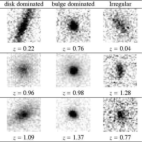	Figure 11: Example of classification in the three main morphological types at different redshifts. The image size is $1.7\hbox {$^\prime $ }\times 1.7\hbox {$^\prime $ }$.
Open with DEXTER

Our results offer the first direct measurement of the distribution of galaxy in three morphological types at $z\simeq1$ from high spatial-resolution imaging in the K-band. We observe that the fraction of $12\%$ of irregular objects at z=1 is significantly higher than the fraction of these objects in the local Universe, confirming from rest-frame data at $\sim$1 microns the well documented trend of this population increasing with redshift (e.g. Brinchmann et al. 1998). However, this result must be taken with caution. Indeed GIM2D accuracy decreases for objects fainter than $K_{\rm s}=19$, which represents $80\%$ of the sample. Moreover at the faint end, the fraction of irregular objects can be overestimated because of the low S/N. But there are good reasons to consider this result significant. Even though there is an over estimation of disks in the faint end, the morphological classification bins are large enough to reduce the number of false classifications. Indeed, even in the zones where the random error in the bulge fraction estimate is $\sim$0.3 or larger, we do not classify a pure bulge ($B/T\sim1$) as a disk.

   
6 Comparison with ground-based and HST observations

In this section we compare our AO observations with ground-based and space observations.

6.1 Ground-based observations

Effective radii of local galaxies, except for compact dwarf galaxies, range from $\sim$1.0 to $\sim$10 kpc depending on their luminosity (Bender et al. 1992; Impey et al. 1996). Our spatial resolution of $\sim$ $0.1\hbox {$^{\prime \prime }$ }$corresponds to about 1 kpc at $z\sim1$ and we should be able to determine morphological types even at z>1. Thus, in order to estimate the performance of AO deep imaging and to justify the automated morphology classification, we compared our images with deep I-band seeing-limited images taken from the Canada-France-Hawaii Telescope Legacy Survey (CFTHLS). One of the so-called deep fields is centered on the COSMOS field, although it is smaller than the total COSMOS area (1 square degree out of 2). Here we used the release T0003 images (March 2006), especially the deep i' one, corresponding to a total integration time of 20 h, with an average FWHM of $\sim$ $0.7\hbox{$^{\prime\prime}$ }$.

We compared real data by selecting a galaxy classified as a disk by GIM2D and C-A in the NACO data and by comparing it to the results obtained with CFHTLS data. We computed the surface brightness profile within the isophotal area enclosed by pixels $3\sigma$ above the sky level. The corresponding limiting surface brightness is $\mu =20$ mag arcsec^-2 for the NACO image and $\mu =25$ mag arcsec^-2 for the MegaCam image. Sky levels and the corresponding isophotal areas were both determined using SE XTRACTOR.

The surface brightness profile was fitted with both a PSF-convolved de Vaucouleurs profile and a PSF-convolved exponential profile. Figure 12 shows that, with seeing-limited observations, it is more difficult to establish a clear separation between both profiles at small distances from the galaxy center (i.e. $\sim$ $0.2\hbox{$^{\prime\prime}$ }$), even if the determination of the brightness profile is possible at much larger distance (i.e. $\sim$ $1\hbox{$^{\prime\prime}$ }$) thanks to the depth of the images and the low noise level of the sky background. This supports the results obtained with GIM2D, which show that a correct estimate of the bulge fraction is possible for small objects. Although ultra-deep sub-arcsecond imaging is powerful in terms of high number statistics, thanks to the wide field coverage, we consider that it is more rewarding to look at a smaller sample of galaxies, but with more reliable morphology determinations thanks to the spatial gain of the AO.

Figure 12: Comparison with ground-based observations. We performed a profile fitting on the same real galaxy observed with NACO ( left) and MegaCam (CFHTLS-i' band, right). The galaxy magnitude is KAB=20.5 and i'=21.3. Surface brightness profiles were computed within the isophotal areas enclosed by pixels $3\sigma$ above the sky level. The corresponding limiting surface brightness is $\mu =20$ mag arcsec-2 for the NACO image and $\mu =25$ mag arcsec-2 for the MegaCam image. The fit was done with a pure de Vaucouleurs and exponential profile.

Open with DEXTER

   
6.2 Space observations

We compare our images with space data taken from the COSMOS survey. Since our observed fields were selected within the COSMOS area, the same objects were observed with the HST-ACS in the I-band at high spatial resolution. We thus morphologically classified the 60 objects for which the photometric redshift are known (Sect. 4). We used those results to both estimate the effect of the observation band on morphology and to validate our method to divide the C/A plane. The C-A estimators were calibrated with simulations using the same method as for the K band data. Standard boundaries, from other existing works, were used to divide the C-A plane. Figure 16 shows the C-A plane cut. The figure also shows the border between bulge-dominated and disk-dominated galaxies obtained with the automatic method described in Sect. 5.2.1 for this population. We again find a negative slope for the border between disk and bulge dominated objects. We find for the whole sample $32\%\pm1.6\%$ irregulars, $47\%\pm1.5\%$ disk-dominated, and $21\%\pm2.5\%$ bulge dominated.

6.2.1 About boundaries

As said, the computed boundaries of the C-A plane are different from what can be found in the literature. Previous works have been done in the I-band using HST imaging (Abraham et al. 1996; Brinchmann et al. 1998). As we have a sample observed in the I-band, we are able to establish whether the change in the boundaries has significant consequences in the morphological classifications. To do so, we classified the I-band sample using the Brinchmann et al. (1998) boundaries and compared the results to the ones obtained with our method (Fig. 14). We find that there are no significant discrepancies between both classifications. We conclude that our method is valid and moreover has the key advantage being free of subjective judgments.

6.2.2 Rest-frame morphologies

We observe some discrepancies in the global morphological distributions between the I and K bands, in particular more perturbed morphologies are seen in the I band. When we look at each object individually (Fig. 13) we confirm this trend: there are uncertainties between K irregulars and I disks and between I disks and K bulges. Indeed an important fraction of bulge-dominated objects and disk-dominated objects detected by NACO are seen as disk-dominated and irregulars respectively, by ACS, as if there was a systematic trend that moves objects to later types when we move to shorter wavelengths. Certainly, the number of objects is small and a few mismatches cause high discrepancies in Fig. 13. However, this is an expected effect since ACS probes younger stellar populations. A visual inspection of some of the objects that present different morphologies reveals that some of the ACS irregulars are in fact well-resolved spiral galaxies with inhomogeneities that probably increase the asymmetry indices.

	Figure 13: Galaxy distribution: comparison between K-band and I band C-A classifications. The figure shows the probability that a galaxy in the K-band is classified in the same morphological type in the I-band.
Open with DEXTER

In order to correctly compare both classifications we need to correct the measurements to estimate how galaxies would look if they were observed locally in the same photometric band. As a matter of fact, Brinchmann et al. (1998) showed that high-z galaxies imaged by HST differ in appearance from their local counterparts because of their reduced apparent size and sampling characteristics, a lower S/N and reduced surface brightness with respect to the sky background and a shift in the rest wavelength of the observations. These effects combine to give some uncertainty in the morphological classifications of galaxies.

	Figure 14: Comparison of classifications with different boundaries. We repeat the morphological classification with the boundaries used by Brinchmann et al. (1998). We conclude that the results do not change significantly which supports the validity of the employed method.
Open with DEXTER

The first effect is a change in the concentration value measured at low redshift. Indeed, Brinchmann et al. (1998) draw the boundaries in the C-A plane using a local sample (Frei et al. 1996) visually classified. However, the concentration value depends on redshift, since the threshold is defined relative to the sky. Thus, less of the galaxy is sampled because of cosmological dimming. The solution they adopt is to correct C for this effect. We do not need a correction of the concentration in this paper because we use simulations that reproduce exactly the observing conditions to calibrate the C-A plane. The result is that boundaries are moved with respect to a local classification instead of changing the C value.

The shift in the rest-frame wavelength of observations is however more difficult to estimate. Indeed the question that arises here is whether the morphological type estimated at high redshift would be the same if observed at low redshift. When observing a galaxy in the K-band at redshift $z\sim1$, the equivalent rest-frame wavelength will be around the z band, however, when observed in the I-band, the rest-frame will be around the B band. That implies that a mismatch can exist in the morphological classification since we are not probing the same morphological blocks. To correct for this effects we need to "move the objects'' into a common rest-frame wavelength. This is the called morphological k correction. The method employed by Brinchmann et al. (1998) consists in determining the morphology from a local sample, redshifting the objects using SED models, and looking at the fraction of galaxies that move in to an other morphological class. A drift coefficient that characterizes the drift from category X to category Y is thus defined as

$$D_{\rm XY}=\frac{N_{\rm X\rightarrow Y}}{N_{\rm X}}\cdot$$ (2)

Once the fraction of missclassified objects is determined, the observed number of objects in class X can be related to the true number:

$$N_{\rm X}^{\rm obs}=N_{\rm X}+\sum{N_{\rm Y}D_{\rm YX}}-N_{\rm X}\sum{D_{\rm XY}}.$$ (3)

Here we proceed as follows: Brinchmann et al. (1998) computed the coefficients to shift from the I observed morphology to the R rest frame morphology, we use those coefficients to correct the observed HST morphology of our sample to the one observed in the R rest frame band, since the filter used for observations is the same (F814W). Once we have this corrected morphology, we can compare it to the NACO uncorrected morphology. This can be done because the observed sample is exactly the same in the K and in the I-band. If we were in the same rest-frame band, we should find the same morphology.

We use the coefficients computed by Brinchmann et al. (1998) to correct the ACS morphology and divide the sample into two redshift bins (z<0.8 and z>0.8). Results are shown in Fig. 15.

• At low redshift (z<0.8) the corrected I-band distributions and the uncorrected K-band are similar. The fact that there is no significant difference between the rest-frame R band and the uncorrected K-band population indicates that, when observing in the K-band, there is no need for morphological k correction.
• At higher redshift, the K-band distribution tends to give a larger fraction of bulge-dominated objects and a lower fraction of irregular objects than the I-band data. This can be caused by the fact that the drift coefficients computed by Brinchmann et al. (1998) might contain errors. Since they are based on SED fitting, it is logical to think that errors are more important for high-redshift objects. This would explain why the results are consistent at low redshift. It can also be a consequence of the size of the sample: as the number of objects per bin is small, errors in the classification of a small fraction can lead to discrepancies between the two bands. This issue will certainly be solved with a larger sample.

Figure 15: Redshift distribution for the three morphological types. We plotted the Brinchmann et al. (1998) sample (circles) and our sample observed with ACS (squares) and with NACO (triangles). Brinchmann et al. (1998) and ACS data are corrected to the R rest-frame band. The NACO sample is observed from the K-band and no correction has been applied. The ACS and NACO samples have been separated into two redshift bins (z<0.8and z>0.8). The represented redshifts are the median redshifts of each bin.

Open with DEXTER

Figure 16: C-A cut for the ACS images. The same classification procedure has been repeated for the same sample observed with ACS in the I-band. Left: simulated objects. Right: real objects. Circles: B/T<0.2, Filled squares: B/T>0.8, crosses: real objects. Dotted line is the border used in Brinchmann et al. (1998) to separate bulge dominated from disk dominated, dashed line is the one computed in the paper.

Open with DEXTER

Table 5: Morphological k correction: morphological differences when observing in the K and I-bands. The same objects observed in the K and I bands present different morphologies. The images size is $1.7\hbox {$^\prime $ }\times 1.7\hbox {$^\prime $ }$.

7 Summary and conclusions

We analyzed the morphologies of a sample of 79 galaxies in the near-infrared thanks to adaptive optics imaging at a resolution of  $0.1\hbox {$^{\prime \prime }$ }$. Thanks to extensive simulations, we showed that adaptive optics can be used to obtain reliable high-resolution 4mm morphological information in an automated way and is thus adapted to large observation programmes:

• Galaxy parameters (bulge fraction, disk scale length, bulge effective radius) can be estimated by means of model fitting with errors lower than $20\%$ up to $K_{\rm s}=19$. This is comparable with space data.
• Galaxies can be separated into three main morphological bins up to $K_{\rm s}=21$, with at least $70\%$ of good identifications and $66\%$ up to $K_{\rm s}=22$.
• For fainter galaxies ( $22<K_{\rm s}<23$) the accuracy of the morphological classification decreases. Simulations show that bulge-dominated and disk-dominated galaxies can be separated with only $55\%$ accuracy at $K_{\rm s}=23$.

We obtain, for the first time, an estimate of the mix of morphological types of the galaxy population up to $z\simeq1$ from ground-based K-band observations with high spatial resolution comparable or better than visible imaging from space. We demonstrate that estimating morphology from K-band data at $z\simeq1$ is not affected by morphological k correction, as there is no significant difference between our population and the corrected I-band population. We find that the fraction of irregulars at $z\simeq1$ is about $12\%\pm2.7\%$ using automated classification methods. This is higher than what is found in local surveys, confirming the well-established trend toward an increasing fraction of irregular galaxies with redshift as observed from surveys in the visible. Our small sample does not allow us to reach firm conclusions on the evolution of the fraction of late-type or early-type galaxies, but classifying galaxies from K-band AO imaging data is demonstrated to be reliable.

From this work it seems clear that adaptive optics can be used for observational cosmology with reliable accuracy, and consequently data of this type should contribute to a better understanding of galaxy evolution in the future. However, it is still a new technique and technical difficulties exist, such as variable PSF, small fields, subsampling and the need of guide stars that make the use of classical reduction methods more difficult. This is now easier with laser guide stars becoming available and new sets of utilities like the ones we are developing to enable easy data processing and analysis of adaptive optics data for the community. This opens the way to observing the large samples required to reach a robust statistical accuracy. We are planning to enlarge our sample by observing a large number of areas around bright stars in the COSMOS field, which will strongly reduce uncertainties in the study of morphological evolution.

Acknowledgements

The authors want to thank the anonymous referee for many useful comments that greatly improved this paper.

References

• Abraham, R., van den Bergh, S., Glazebrook, K., et al. 1996, ApJS, 107, 1 [NASA ADS] [CrossRef]
• Abraham, R. G., Valdes, F., Yee, H. K. C., & van den Bergh, S. 1994, ApJ, 432, 75 [NASA ADS] [CrossRef] (In the text)
• Abraham, R. G., van den Bergh, S., & Nair, P. 2003, ApJ, 588, 218 [NASA ADS] [CrossRef]
• Baker, A. J., Davies, R. I., Lehnert, M. D., et al. 2003, A&A, 406, 593 [NASA ADS] [CrossRef] [EDP Sciences] (In the text)
• Baugh, C. M., Cole, S., & Frenk, C. S. 1996, MNRAS, 283, 1361 [NASA ADS]
• Bender, R., Burstein, D., & Faber, S. M. 1992, ApJ, 399, 462 [NASA ADS] [CrossRef]
• Bershady, M. A., Lowenthal, J. D., & Koo, D. C. 1998, ApJ, 505, 50 [NASA ADS] [CrossRef]
• Bertin, E., & Arnouts, S. 1996, A&AS, 117, 393 [NASA ADS] (In the text)
• Brinchmann, J., & Ellis, R. S. 2000, ApJ, 536, L77 [NASA ADS] [CrossRef]
• Brinchmann, J., Abraham, R., Schade, D., et al. 1998, ApJ, 499, 112 [NASA ADS] [CrossRef]
• Bundy, K., Ellis, R. S., & Conselice, C. J. 2005, ApJ, 625, 621 [NASA ADS] [CrossRef]
• Cole, S., Lacey, C. G., Baugh, C. M., & Frenk, C. S. 2000, MNRAS, 319, 168 [NASA ADS]
• Conselice, C. J., Bershady, M. A., & Jangren, A. 2000, ApJ, 529, 886 [NASA ADS] [CrossRef] (In the text)
• Cowie, L. L., Songaila, A., Hu, E. M., & Cohen, J. G. 1996, AJ, 112, 839 [NASA ADS] [CrossRef]
• Cresci, G., Davies, R., Baker, F., et al. 2006 [arXiv:astro-ph/0607221] (In the text)
• De Lucia, G., Springel, V., White, S. D. M., Croton, D., & Kauffmann, G. 2006, MNRAS, 366, 499 [NASA ADS]
• de Vaucouleurs, G. 1948, Annales d'Astrophysique, 11, 247 [NASA ADS]
• Fall, S. M., & Efstathiou, G. 1980, MNRAS, 193, 189 [NASA ADS] (In the text)
• Frei, Z., Guhathakurta, P., Gunn, J. E., & Tyson, J. A. 1996, AJ, 111, 174 [NASA ADS] [CrossRef] (In the text)
• Gardner, J. P. 1998, PASP, 110, 291 [NASA ADS] [CrossRef] (In the text)
• Gardner, J. P., Cowie, L. L., & Wainscoat, R. J. 1993, ApJ, 415, L9 [NASA ADS] [CrossRef]
• Glazebrook, K., Peacock, J. A., Miller, L., & Collins, C. A. 1995, MNRAS, 275, 169 [NASA ADS]
• Hubble, E. 1936, ApJ, 415
• Ilbert, O., Arnouts, S., McCracken, H. J., et al. 2006a, ArXiv Astrophysics e-prints (In the text)
• Ilbert, O., Lauger, S., Tresse, L., et al. 2006b, A&A, 453, 809 [NASA ADS] [CrossRef] [EDP Sciences]
• Impey, C. D., Sprayberry, D., Irwin, M. J., & Bothun, G. D. 1996, ApJS, 105, 209 [NASA ADS] [CrossRef]
• Kleinmann, S. G. 1992, in Robotic Telescopes in the 1990s, ed. A. V. Filippenko, ASP Conf. Ser., 34, 203 (In the text)
• Lilly, S., & The Zcosmos Team. 2006, ApJ, in press (In the text)
• Lilly, S. J., Le Fevre, O., Hammer, F., & Crampton, D. 1996, ApJ, 460, L1 [NASA ADS] [CrossRef]
• Madau, P., Pozzetti, L., & Dickinson, M. 1998, ApJ, 498, 106 [NASA ADS] [CrossRef]
• Maihara, T., Iwamuro, F., Tanabe, H., et al. 2001, PASJ, 53, 25 [NASA ADS]
• McCracken, H. J., Metcalfe, N., Shanks, T., et al. 2000, MNRAS, 311, 707 [NASA ADS]
• McLeod, B. A., Bernstein, G. M., Rieke, M. J., Tollestrup, E. V., & Fazio, G. G. 1995, ApJS, 96, 117 [NASA ADS] [CrossRef]
• Mignoli, M., Cimatti, A., Zamorani, G., et al. 2005, A&A, 437, 883 [NASA ADS] [CrossRef] [EDP Sciences] (In the text)
• Minowa, Y., Kobayashi, N., Yoshii, Y., et al. 2005, ApJ, 629, 29 [NASA ADS] [CrossRef] (In the text)
• Persson, S. E., Murphy, D. C., Krzeminski, W., Roth, M., & Rieke, M. J. 1998, AJ, 116, 2475 [NASA ADS] [CrossRef] (In the text)
• Sandage, A. 1961, The Hubble atlas of galaxies (Washington: Carnegie Institution)
• Scoville, N. Z., & COSMOS Team. 2005, in BAAS, 1309 (In the text)
• Simard, L., Willmer, C. N. A., Vogt, N. P., et al. 2002, ApJS, 142, 1 [NASA ADS] [CrossRef]
• Vapnik, V. 1995, Springer-Verlag, 536 (In the text)
• Wolf, C., Meisenheimer, K., Rix, H.-W., et al. 2003, A&A, 401, 73 [NASA ADS] [CrossRef] [EDP Sciences]
• Zucca, E., Ilbert, O., Bardelli, S., et al. 2006, A&A, 455, 879 [NASA ADS] [CrossRef] [EDP Sciences]

 

  
Online Material

Table 6: Summary of the morphological classifications for the 79 detected objects. For each object we show the I and K band magnitudes and the estimated morphological type from AO imaging in the K-band (with GIM2D and C-A) and from HST-ACS in the I-band. BD stands for bulge-dominated, DD for disk-dominated and I for irregular.

   
Appendix A: Galaxy number counts

The number densities of galaxies as a function of magnitude is a classical test of evolutionary and large-scale structure models (McCracken et al. 2000). Number counts can help to constrain the Universe models, and may provide constraints on the globally-averaged initial mass function. In order to make reliable measurements and compare them with previous ones, we apply several corrections to the raw numbers. Firstly we correct for completeness using the computed completeness for extended sources (see Fig. 4). Completeness changes as a function of the galaxy morphological type; we thus use the bulge fraction computed with GIM2D (see Sect. 5.2.2) to estimate the completeness for each detected galaxy. In that way, a galaxy with a detection probability $P_{\rm det}$, will be counted as $1/P_{\rm det}$. In a second step, the number counts might also contain the counts from spurious detections due to the effect of statistical noise that becomes significant in the faint end. Those spurious detections are removed using the MAG_AUTO/MU_MAX plane as explained above (Fig. 2). Stellar objects are also removed at this step. Finally, errors in the determination of the object's photometry might result in a scatter of galaxy number counts among magnitude bins. In order to evaluate this effect we generated the probability matrix P_ijthat gives the probability that an artificial object detected with magnitude m_iactually has a magnitude of m_j. We corrected the galaxy number counts accordingly. The results of our galaxy number counts are shown in Fig. A.1.

Figure A.1: Ks corrected number counts compared with other K-band surveys. The solid line is the best fitting power-law in the range $17<K_{\rm s}<22$, with a slope ${\rm d}\!\log~(N)/{\rm d}m=0.42\pm0.05$. Error bars show poissonian errors.

We perform galaxy number counts up to $K_{\rm s}=22$. Above this magnitude limit, counts are no longer reliable as they must be corrected by a factor as large as the uncertainties; they are consequently not represented. We compute a power-law fitting in the range $17<K_{\rm s}<22$ since the K-band number counts tend to show a slope change at $K\sim17$ (Gardner et al. 1993). We find a mean slope of ${\rm d}(\log N)/{\rm d}m=0.42\pm0.05$, which is in good agreement with previous works (Bershady et al. 1998; McCracken et al. 2000). This slope is however much larger than the one derived from the SWAN observations (Cresci et al. 2006), also performed with an adaptive optics system. Indeed they claim to find a mean slope of ${\rm d}(\log N)/{\rm d}m=0.26\pm0.01$ in the range $16<K_{\rm s}<22$. As stated in Baker et al. (2003), the SWAN fields present, however, a selection bias at the bright end, since the fields were chosen to have an excess of bright galaxies. This could explain this difference despite that the excess becomes significant at $K_{\rm s}<16$, which is out of the computation range.