 |
(1) |
A&A 468, 313-321 (2007)
DOI: 10.1051/0004-6361:20054495
A. Otto1 - J. Büchner2 - B. Nikutowski2
1 - Geophysical Institute, University of Alaska, Fairbanks, AK 99775,
USA
2 - Max-Planck-Institut für Sonnensystemforschung, Max-Planck-Str.
2, 37191, Katlenburg-Lindau, Germany
Received 8 November 2005 / Accepted 14 February 2007
Abstract
Context. In recent years the accuracy of magnetic field observations in the solar atmosphere has made considerable progress. Similar progress is being made in computer modeling of complex plasma systems and computer capabilities.
Aims. To consider observed solar magnetic field structure in numerical simulations a new extrapolation method for solar magnetic fields is used to incorporate such fields into three-dimensional MHD simulations
Methods. The simulation employs a new modified linear magnetic field extrapolation which is specifically designed to satisfy symmetry conditions which are generic to MHD models. The model domain includes photosphere, chromosphere, and corona.
Results. The new model is applied to several solar field configurations and results are compared to three-dimensional field structure from observations and another extrapolation method. The new model provides a simple and efficient method for the simulation of observed solar magnetic field structures by constructing a three-dimensional initial field that is consistent with symmetry boundary conditions of MHD simulations.
Key words: magnetohydrodynamics (MHD) - Sun: magnetic fields - Sun: corona - methods: numerical - plasmas
Modern investigations of the solar atmosphere provide a wealth of new information on the magnetic and plasma structure. A valuable tool to interpret these data is numerical simulation of the magnetic coupling between the different regions of the solar atmosphere starting from the photosphere, where the magnetic field can be determined with the highest spatial resolution, through the chromosphere and the corona.
Existing solar simulation models usually use model magnetic fields on meso-scales (e.g., Choe & Cheng 2002; Cheng et al. 2003; Galsgaard et al. 2003; Antiochos et al. 2002; Priest & Forbes 2000) or address global solar phenomena (e.g., Linker et al. 2001; Mikic et al. 1999; Linker et al. 2003) to investigate the influence of the photospheric boundary conditions such as magnetic shear, plasma motion, emerging flux, etc. A first meso-scale simulation model based on observed line of sight magnetic fields has been used by Gudiksen & Nordlund (2002) to study coronal heating. The further development of such models is highly desirable to interpret the properties and evolution of structures in the solar atmosphere as observed in various wavelengths of the solar radiation. Here we describe a new method to incorporate observed photospheric magnetic fields in magnetohydrodynamic simulations to study the evolution of solar magnetic fields. For applications we refer to other publications (Büchner et al. 2005b,2004,2005a)
The method consists of two parts. First, the observed magnetic field
along the direction of the line of sight has to be converted into
three-dimensional magnetic fields. Our approach employs a solution
of the force free magnetic field condition
 (we use
instead of
the common
(we use
instead of
the common  the latter is used as an angular variable in
the Fourier expansion in this paper). Although there are various linear
and nonlinear methods for the extrapolation of solar magnetic field
most of these are not suitable to be used as initial conditions for
MHD simulations because of the required MHD boundary conditions.
the latter is used as an angular variable in
the Fourier expansion in this paper). Although there are various linear
and nonlinear methods for the extrapolation of solar magnetic field
most of these are not suitable to be used as initial conditions for
MHD simulations because of the required MHD boundary conditions.
The second step consists of the use of the extrapolated magnetic fields as an initial condition in the MHD simulation. The simulation code uses a finite difference approximation for the full set of MHD equations where the plasma is coupled to a neutral fluid. The latter is important in the photosphere and chromosphere.
The following section focuses on the extrapolation of the magnetic field consistent with MHD boundary conditions. Properties of the initial state and the extrapolated magnetic field for a case of a coronal bright point analyzed by Brown et al. (2001) are discussed in Sect. 3. Section 4 addresses the simulation method and the last section presents a summary and discussion of the presented results.
Various methods have been suggested to derive three-dimensional magnetic
field structures from the line-of-sight magnetic field component.
Several of these methods use potential (Semel 1968; Schmidt 1964), linear
(Semel 1988; Seehafer 1978; Chiu & Hilton 1977), or nonlinear force free fields
(Cuperman et al. 1990; Amari et al. 1997; Aly 1989) with a non-constant value of the
force-free parameter .
The use of the extrapolated fields
for MHD simulations, however, requires that the boundary conditions
of the extrapolation are consistent with boundary conditions that
can be applied to the MHD simulation. For the purpose of constructing
a method which can easily be employed and automated to construct three-dimensional
magnetic equilibria a constant value
is the most straightforward
choice. The particular numerical value of
can always be
chosen to represent characteristics of the observed magnetic field
such as the stretching with altitude over the photosphere or a particular
(inferred) magnetic helicity.
Our approach uses a method similar to the one outlined by Seehafer (1978).
This solution is constructed through a Fourier series expansion of
the magnetic field components where the coefficients of the horizontal
components (Bx and By) are related to the vertical component
z component Bz through the force free condition (1)
and
 .
This procedure implies periodic solutions
in the x and y directions. The solution of Seehafer (1978) has
the particular advantage of using a symmetry condition for Bzat the x and y boundaries of the system which allow a solution
in a quarter of the full periodic system, i.e., the solution is constructed
in the domain
.
This procedure implies periodic solutions
in the x and y directions. The solution of Seehafer (1978) has
the particular advantage of using a symmetry condition for Bzat the x and y boundaries of the system which allow a solution
in a quarter of the full periodic system, i.e., the solution is constructed
in the domain
 ,
,
 while the
full period covers the domain
while the
full period covers the domain
 ,
,
 .
This avoids the need for periodicity in the magnetic field.
.
This avoids the need for periodicity in the magnetic field.
However, this solution is not suitable as an initial condition for
an MHD simulation which requires well defined symmetry conditions
at the boundaries. For Bz the solution by Seehafer (1978) employs

 such that
Bz(0,y,z)=Bz(x,0,z)=0.
such that
Bz(0,y,z)=Bz(x,0,z)=0.
Using proper MHD symmetry boundary conditions (a detailed
discussion will be given in the following section) at x=0 implies
either
Bx(-x,y,z)=-Bx(x,y,z) or
Bx(-x,y,z)=Bx(x,y,z).
Allowing for a non vanishing normal component at this boundary therefore
implies the second choice. Furthermore
requires
 at the x=0 boundary (
 ,
and
,
and
 )
which
can only be satisfied in general if
By(-x,y,z)=-By(x,y,z)or
By(0,y,z)=0. Thus the normal component Bx is symmetric
and nonzero while the tangential components are zero and reverse sign.
However, using these symmetries and calculating the current at the
boundary x=0 yields
)
which
can only be satisfied in general if
By(-x,y,z)=-By(x,y,z)or
By(0,y,z)=0. Thus the normal component Bx is symmetric
and nonzero while the tangential components are zero and reverse sign.
However, using these symmetries and calculating the current at the
boundary x=0 yields
 .
Thus the normal component of the current must reverse sign at the
boundary.
.
Thus the normal component of the current must reverse sign at the
boundary.
The other boundaries at x and y have the same symmetry conditions. While there is no problem in the interior domain the conditions at the x and y boundaries are in contradiction to the force free condition (1) because the magnetic field normal to the boundary is continuous and the current normal to the boundary reverses sign. The reason for this mismatch is that the symmetry boundary condition is not the proper continuation of the magnetic field into the region x<0. The proper continuation into this region is determined by the fully periodic solution from -Lx to +Lx. For this reason the solution by Seehafer (1978) is not suitable as initial condition for an MHD simulation because an MHD simulation requires boundary conditions which are local symmetry conditions or requires to consider the full period of the system as considered by Gudiksen & Nordlund (2002). However, as will be illustrated the approach by Seehafer (1978) can be modified to accommodate well defined MHD symmetry conditions.
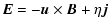
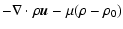
The MHD simulation will use the full set of MHD equations
![$x=\left[0,L_{x}\right]$](/articles/aa/full/2007/22/aa4495-05/img31.gif) and
y=[-Ly/2,Ly/2]. We will now consider symmetry
conditions at the boundary x=0 for a plane
and distinguish two basic cases:
,
and
y=[-Ly/2,Ly/2]. We will now consider symmetry
conditions at the boundary x=0 for a plane
and distinguish two basic cases:
,
 ,
and
,
and
 ,
which implies
,
which implies
 ,
,
 ,
and
,
and
 where
where
 .
.
The MHD variables must transform such that the MHD equations remain
invariant for the transformation implied by the boundary condition.
There are two possibilities for the individual variables. They can
transform either as
f(-x,y,z)=f(x,y,z) which we call symmetric
(abbreviated "s'') or they may transform as
g(-x,y,z)=-g(x,y,z)which we call antisymmetric (or "a''). Positive definite variables
like  ,
p, and
,
p, and  must transform symmetric for instance
 .
Examining the full set of MHD equation
with these rules yields two possible sets of transformations which
maintain the invariance of the equations. The result for the individual
variables is summarized in Table 1.
.
Examining the full set of MHD equation
with these rules yields two possible sets of transformations which
maintain the invariance of the equations. The result for the individual
variables is summarized in Table 1.
Table 1:
Transformation properties for the transformation
,
,
and
.
The result demonstrates that the transformation of the magnetic field components is always different than the transformation of the current density components. Set "a'' is not suitable because of the reasons outlined above. Set "b'' implies a zero normal magnetic field (at x=0) but has a nonzero normal current density which is also inconsistent with the force free condition (1).
,
 ,
and
,
which implies
,
,
and
,
which implies
,
 ,
and
,
and
 .
This resulting set of
boundary conditions implies a line symmetry along the line x=y=0.
.
This resulting set of
boundary conditions implies a line symmetry along the line x=y=0.
Similar to the prior symmetry all positive definite MHD variables
must be symmetric, e.g.,
 .
The result
for all variables is given in Table 2.
.
The result
for all variables is given in Table 2.
Table 2:
Transformation properties for the transformation
,
,
and
.
Both set "a'' and set "b'' have the same transformation properties for
the magnetic field and the current density and are thus suitable for
the MHD equations satisfying the force-free condition. In the following
we will employ the transformation set "b'' for the magnetic field extrapolation.
Note that while for MHD models the symmetry set (a) is equally suitable
but is lost if the Hall term is included in Ohm's law. The boundary
condition has some implications regarding a preconditioning of the
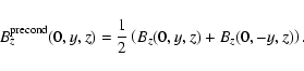
initial magnetic field. The symmetry also applies to the plane x=0,
i.e.,
Bz(0,-y,z)=Bz(0,y,z) such that the magnetic field
along the z axis must be symmetric with respect to y=0 which
can be obtained through
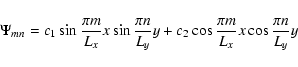
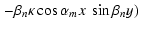
In the x, y plane we assume an expansion for Bz with base
functions of the form

![\begin{figure}
\par\includegraphics[width=7.1cm,clip]{4495f1.eps}
\end{figure}](/articles/aa/full/2007/22/aa4495-05/img53.gif) |
Figure 1: Illustration of the geometry of line symmetry. |
| Open with DEXTER | |
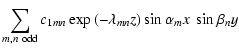
The solution is found similar to the work by Seehafer using an expansion
in the form:
 ,
,
 ,
and
,
and
 .
A given polarity
image in Bz is expanded in the set of these base functions at
the solar surface z=0 subject to the preconditioning of the image
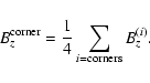
data according to (6) and (7). The extrapolated
solution is then used as an initial condition in the full three-dimensional
MHD simulation model.
.
A given polarity
image in Bz is expanded in the set of these base functions at
the solar surface z=0 subject to the preconditioning of the image
data according to (6) and (7). The extrapolated
solution is then used as an initial condition in the full three-dimensional
MHD simulation model.
It is important to note that neither the Seehafer (1978) nor the presented method require a total magnetic flux balance different from a fully periodic solution as used by Gudiksen & Nordlund (2002). The Seehafer (1978) solution is restricted in that it requires that the magnetic field has only a normal component at the boundaries in x and y while our extrapolation allows that all components of the magnetic field are non-zero at these boundaries except for the lines of symmetry.
The goal of the magnetic field extrapolation is to construct a suitable initial condition for an MHD simulation of the corresponding configuration. This does not necessarily imply that the initial configuration has to reflect the exact state of the magnetic field at the start of the simulation because this configuration undergoes continuous changes caused by the photospheric plasma motion. For this reason the magnetic and plasma structure can never be expected to be in an exact equilibrium configuration. However, after sufficient time has passed it can reasonably be expected that the precise initial state has only a minor influence on the dynamical evolution. In other words the system has a finite memory.
![\begin{figure}
\par\includegraphics[width=8.3cm,clip]{4495f2.eps}
\end{figure}](/articles/aa/full/2007/22/aa4495-05/img71.gif) |
Figure 2:
Magnetogram of the line of sight components at
the beginning of the  phase of an observed EUV bright point (Brown et al. 2001). phase of an observed EUV bright point (Brown et al. 2001). |
| Open with DEXTER | |
Nevertheless, it is desirable that basic geometrical magnetic field properties are accurately reflected in the initial magnetic field. Boundary conditions always influence this geometry and the magnetic field evolution. Therefore it is important to choose a simulation domain of sufficient size such that the main magnetic field concentrations and their inter-connections are contained within the system. As an example for the model properties we used a magnetogram related to an EUV bright point described by Brown et al. (2001). The original magnetogram is shown in Fig. 2 with a pixel size of about 500 km. We note that a decomposition by 32 modes provides a highly accurate representation of the original magnetogram. However, for a system size of 28 Mm as in the case of the Brown et al. (2001) observation, the scale height of harmonics larger than 16 is less than 600 km, decreasing with increasing mode number. Thus the higher order harmonics do not contribute significantly to the magnetic field structure at transition region heights and in the solar corona.
![\begin{figure}
\par\includegraphics[width=6.9cm,clip]{4495f3a.eps}\par\vspace*{2mm}
\includegraphics[width=6.9cm,clip]{4495f3b.eps}
\end{figure}](/articles/aa/full/2007/22/aa4495-05/img72.gif) |
Figure 3: Representation of the magnetogram in Fig. 2 by 16 ( top) and by 8 Fourier modes ( bottom) with an overlay of magnetic field lines representing the potential field. Field lines are started from the photospheric boundary and projected onto this boundary. |
| Open with DEXTER | |
The Fourier decomposed Bz magnetic field component based on
the solution in described in Sect. 2.3 for
 is shown in Fig. 3. Here the magnetogram
is resolved by 8 and by 16 Fourier modes for each direction. The plots
also include the projection of magnetic field lines starting from
the photospheric boundary where a reddish color indicates field lines
extending higher into the photosphere. Both decompositions show the
main magnetic polarities of the original data albeit the size of the
major polarities increases with decreasing mode number and the magnitude
of the magnetic field decreases with decreasing mode number. Although
magnetic field lines have some similarity Fig. 3
demonstrates that the inclusion of higher harmonics describes more
complex details of the field structure. Also more of the uniformly
space field lines are short and close within the photosphere consistent
with the small scale height of higher harmonics.
is shown in Fig. 3. Here the magnetogram
is resolved by 8 and by 16 Fourier modes for each direction. The plots
also include the projection of magnetic field lines starting from
the photospheric boundary where a reddish color indicates field lines
extending higher into the photosphere. Both decompositions show the
main magnetic polarities of the original data albeit the size of the
major polarities increases with decreasing mode number and the magnitude
of the magnetic field decreases with decreasing mode number. Although
magnetic field lines have some similarity Fig. 3
demonstrates that the inclusion of higher harmonics describes more
complex details of the field structure. Also more of the uniformly
space field lines are short and close within the photosphere consistent
with the small scale height of higher harmonics.
In comparison to our 8 mode solution Fig. 4 shows the Seehafer (1978) extrapolation with 8 modes. The two results show very similar distributions of the polarities and a similar shape of field lines close to the center of the system. However, field lines close to the boundary are rather different. The figure also demonstrates that all boundary field lines in the Seehafer solution are normal to the boundaries where they leave the domain as expected by the symmetry conditions discussed in Sect. 2. In fact the extrapolation after Seehafer (1978) allows only a normal component of the magnetic field at the boundary.
![\begin{figure}
\par\includegraphics[width=6.9cm,clip]{4495f4.eps}
\end{figure}](/articles/aa/full/2007/22/aa4495-05/img74.gif) |
Figure 4: Same as Fig. 3 for the Seehafer (1978) 8 mode extrapolation. |
| Open with DEXTER | |
The difference in the Bz component between our extrapolation and the Seehafer extrapolation is shown in Fig. 5 for the 16 mode expansion. The largest differences occur close to the boundaries as can be expected because of the different boundary conditions. The differences are also most pronounced in the highest order modes indicating that the difference decreases fast with height.
![\begin{figure}
\par\includegraphics[width=8.4cm,clip]{4495f5.eps}
\end{figure}](/articles/aa/full/2007/22/aa4495-05/img75.gif) |
Figure 5: Difference of the line of sight magnetic field between the Seehafer and our extrapolation for 16 modes. |
| Open with DEXTER | |
However, the comparison of the extrapolated magnetic fields does not
necessarily imply that the magnetic structure is similar. A quantitative
measure of this structure is difficult and the comparison of individual
field lines is a poor indicator of the basic field structure because
magnetic flux boundaries can be shifted by a small amount such that
individual magnetic flux tubes started at the same physical location
can have entirely different shape. Here we employ the differential
magnetic flux tube volume
![\begin{figure}
\par\includegraphics[width=8.2cm,clip]{4495f6.eps}
\end{figure}](/articles/aa/full/2007/22/aa4495-05/img77.gif) |
Figure 6: Flux tube volume for our magnetic field extrapolation ( top) and Seehafer's model. |
| Open with DEXTER | |
The differential magnetic flux tube volume for our field model and for the Seehafer extrapolation is shown in Fig. 6 for the cases of 8 modes and 16 modes for our model and the 8 mode expansion for the Seehafer model. Comparison with Fig. 3 demonstrates that small flux tube volume is indicative for short flux tubes which close below the transition region. These are typically arranged along polarity inversion boundaries. Large flux tube volume indicates foot point locations of magnetic structures which rise to considerable height. Large flux tube volume can also be indicative for complex magnetic structure because the differential flux tube volume becomes very large (or diverges) close to magnetic neutral points or lines.
The comparison of the 8 mode expansions show good agreement in the
central region of the system whereas there are considerable differences
closer to the boundaries. Noticeable are very large flux tube volumes
close to the boundaries in the Seehafer extrapolation. It turns out
that these are actually an artifact of the Seehafer solution. Since
the potential field in this expansion has only a normal component
at the boundaries, any change of the polarity of the normal component
implies a zero value of the magnetic field. Thus a reversal of the
normal component implies the presence of artificial neutral lines
at these boundaries. Figure 7 shows the normal magnetic
field and the neutral lines for the Seehafer extrapolation at the
x=0 boundary.
![\begin{figure}
\par\includegraphics[width=7.9cm,clip]{4495f7.eps}
\end{figure}](/articles/aa/full/2007/22/aa4495-05/img78.gif) |
Figure 7: Normal magnetic field for the Seehafer solution at x=0. |
| Open with DEXTER | |
A generic topological property of a three-dimensional field are isolated neutral points rather than neutral lines. Thus our model contains only isolated neutral points. The area of photospheric regions which map into the vicinity of neutral points is small. In contrast the presence of neutral lines (rather than neutral points) at the boundaries of the Seehafer extrapolation leads to the extended photospheric regions of large magnetic flux tube volumes illustrated in Fig. 6.
The 8 mode plot in Fig. 6 shows a relatively simple structure where areas with bluish color indicate longer field lines extending into the corona or mapping to the vicinity of neutral points. The case of 16 modes shows the same basic structure, however, with smaller dark regions which are cut out of the regions of higher flux tube volume. To understand this one has to remember that a larger number of modes implies the presence of small scale structure which also has a small scale height, i.e., which is not reaching into the corona. The strong magnetic field regions are more confined for cases with larger mode numbers. The dark cutouts in the flux tube volume reflect these small loops that do not reach into the corona and therefore have small flux tube volume. The same tendency, i.e., additional small size cutouts from the larger flux tube volume regions continuous in the case of 32 or more modes (not shown).
Another important question is the deviation of the tangential (Bxand By) components of the magnetic field, which arise in both,
the Seehafer and our extrapolation methods although they start with
the normal (Bz) component of the photospheric magnetic field
alone. The reason is that the force-free condition
 requires for selfconsistency finite Bx and By components
as well. In order to test our new extrapolation method we applied
it to a case, where the full vector magnetogram information was available.
As such we choose the active region NOAA AR8210 which was previously
discussed and investigated in detail by Longcope (2004) and Welsch et al. (2004).
We choose the moment 17:30 UT, just before a major eruption took place.
As a quantitative measure for the deviation we calculated the relative
tangential magnetic field deviation
requires for selfconsistency finite Bx and By components
as well. In order to test our new extrapolation method we applied
it to a case, where the full vector magnetogram information was available.
As such we choose the active region NOAA AR8210 which was previously
discussed and investigated in detail by Longcope (2004) and Welsch et al. (2004).
We choose the moment 17:30 UT, just before a major eruption took place.
As a quantitative measure for the deviation we calculated the relative
tangential magnetic field deviation
 ,
i.e., potential fields. Both methods reveal similar regions
with deviations in the tangential magnetic field components as compared
to the observed ones. Because of the similarity we interpret most
regions with large deviations as regions where larger field-aligned
(and possibly perpendicular ) currents are present in the observed
fields. Both methods also indicate larger deviations close to the
boundaries which is expected because of the influence of the boundary
conditions on the solution.
,
i.e., potential fields. Both methods reveal similar regions
with deviations in the tangential magnetic field components as compared
to the observed ones. Because of the similarity we interpret most
regions with large deviations as regions where larger field-aligned
(and possibly perpendicular ) currents are present in the observed
fields. Both methods also indicate larger deviations close to the
boundaries which is expected because of the influence of the boundary
conditions on the solution.
![\begin{figure}
\par\includegraphics[width=8.3cm,clip]{4495f8.eps}
\end{figure}](/articles/aa/full/2007/22/aa4495-05/img81.gif) |
Figure 8: Deviation of the tangential magnetic field between the extrapolated (our model - top; Seehafer - bottom) field and the vector magnetogram for the active region NOAA AR8210. |
| Open with DEXTER | |
The MHD equations are solved with a Leapfrog scheme which is second order accurate and has very low dissipation. A small dissipation is switched on if oscillations develop on the grid scale similar to flux corrected transport (FCT) schemes. Terms involving second order derivatives are treated with the Dufort-Frankel method which allows to consider very small resistivity.
The grid is chosen nonuniform in the z direction with the highest
resolution at  and
and
 (corresponding to about
160 km). At least 8 grid points should be considered for the smallest
wave lengths of the Fourier series expansion to ensure sufficiently
small discretization errors for the finite difference scheme, i.e.,
for an area of 64 pixels modeled with a maximum of 8 modes per direction
at least 64 grid points should be used for the simulation. In fact
it turned out that 16 grid points are desirable for the shortest wavelength
of the 16 mode expansion examples presented here. This corresponds
to a
(corresponding to about
160 km). At least 8 grid points should be considered for the smallest
wave lengths of the Fourier series expansion to ensure sufficiently
small discretization errors for the finite difference scheme, i.e.,
for an area of 64 pixels modeled with a maximum of 8 modes per direction
at least 64 grid points should be used for the simulation. In fact
it turned out that 16 grid points are desirable for the shortest wavelength
of the 16 mode expansion examples presented here. This corresponds
to a
 grid in the x, y plane. Since magnetic flux and
energy decrease fast with with altitude, only modes which contribute
significantly at coronal heights (z>4) are important for reconnection
and magnetic reconfiguration in the corona.
grid in the x, y plane. Since magnetic flux and
energy decrease fast with with altitude, only modes which contribute
significantly at coronal heights (z>4) are important for reconnection
and magnetic reconfiguration in the corona.
An important consideration for a model of the photosphere/chromosphere/corona region is the interaction with the neutral environment. In the collision dominated photosphere and chromosphere this implies ionization and recombination, friction, and thermal contact between the plasma and neutrals. Radiative processes are not included in the present model. The plasma is coupled to a neutral background fluid which is present only in the lower (z<4) portion of the system representing photosphere and chromosphere.
The focus of the current implementation of the model is to provide
a framework to simulate solar processes based on the extrapolation (Sect. 2)
of observed photospheric magnetic field and to examine basic effects
caused by the collisional environment below the transition region.
 because this yields a continuity equation in the absence of source
terms for the internal energy.
because this yields a continuity equation in the absence of source
terms for the internal energy.
The above set of equations is in normalized units. We normalize magnetic
field to
 ,
plasma density to
the density in the corona just above the transition region
,
plasma density to
the density in the corona just above the transition region
 m-3for protons (the actual number density is smaller but a presence of
heavier ions and convenience let us choose this number), and length
scales close to the length of an MDI pixel size L0=500 km.
This yields a normalization of velocities to the Alfvén speed
m-3for protons (the actual number density is smaller but a presence of
heavier ions and convenience let us choose this number), and length
scales close to the length of an MDI pixel size L0=500 km.
This yields a normalization of velocities to the Alfvén speed
 km s-1 and of times to Alfvén times
 s.
Pressure is normalized to typical magnetic pressure
s.
Pressure is normalized to typical magnetic pressure
 and temperature to
 (the factor 2 is because of electrons and ions). This yields a typical
thermal velocity of
(the factor 2 is because of electrons and ions). This yields a typical
thermal velocity of
 .
Note that the physical temperature
.
Note that the physical temperature  is determined by
 with p and
being the pressure and plasma mass density (assuming
protons) in simulation units.
with p and
being the pressure and plasma mass density (assuming
protons) in simulation units.
The ion neutral collision frequency is
 with
with
 m2. In normalized units this
yields
m2. In normalized units this
yields
 ,
where
,
where  is the neutral
mass density normalized to
is the neutral
mass density normalized to  (assuming hydrogen). This illustrates
that the normalized collision frequency is large anywhere below the
transition region (increasing toward the solar surface).
(assuming hydrogen). This illustrates
that the normalized collision frequency is large anywhere below the
transition region (increasing toward the solar surface).
Electron - ion collision frequencies are about
 s-1in the photosphere/chromosphere and
 s-1in the lower corona. The normalized resistivity is
 with the electron inertia length
 .
Note
that the diffusion time is
.
Note
that the diffusion time is
 which is 107 s in the photosphere/chromosphere and 1010 s
in the corona. The corresponding normalized resistivity is between
which is 107 s in the photosphere/chromosphere and 1010 s
in the corona. The corresponding normalized resistivity is between
 and
and
 .
However, the classical
resistivity is far too small to explain observed time-scales of reconnection
in the solar corona. In the simulation model we use a current dependent
resistivity based on the drift speed of the current carriers. Our
model assumes particle scattering as a result of plasma turbulence
when the drift velocity surpasses a threshold value (such as for ion-acoustic
or other micro-instabilities). Since these are sub grid processes
it is assumed that the actual current are filamentary and on a scale
of a few km, i.e. about 1/100 of our horizontal grid resolution. The
resistivity is switched on when the parallel plasma velocity is larger
then some critical value (
.
However, the classical
resistivity is far too small to explain observed time-scales of reconnection
in the solar corona. In the simulation model we use a current dependent
resistivity based on the drift speed of the current carriers. Our
model assumes particle scattering as a result of plasma turbulence
when the drift velocity surpasses a threshold value (such as for ion-acoustic
or other micro-instabilities). Since these are sub grid processes
it is assumed that the actual current are filamentary and on a scale
of a few km, i.e. about 1/100 of our horizontal grid resolution. The
resistivity is switched on when the parallel plasma velocity is larger
then some critical value (
 )
where
)
where
 is the height of the transition region.
Note that for strong magnetic fields the resistivity and Alfvén time decrease with the inverse magnitude of the magnetic field. To obtain fast reconnection the thickness of the diffusion region has to decrease to about 1 km below the transition region (if fast reconnection were possible with the strong neutral coupling) and to about 1 m in the corona (and below these values if the magnetic field is larger than B0=1 G).
The value for the ion neutral collision frequency is chosen in part
for numerical reasons (very large collision frequencies may require to
reduce the time step). The mass density below the transition region is
assumed to increase to  (in units of the corona density
which is set to 1) and the normalized collision frequency is assumed
with a maximum of
(in units of the corona density
which is set to 1) and the normalized collision frequency is assumed
with a maximum of  in the photosphere. This underestimates the
actual collisional effects such as friction, however, whether the
plasma is forced with 99% of the neutral velocity or with 99.99% is
not significant for the physics. On the considered time scales the
forcing is always large.
in the photosphere. This underestimates the
actual collisional effects such as friction, however, whether the
plasma is forced with 99% of the neutral velocity or with 99.99% is
not significant for the physics. On the considered time scales the
forcing is always large.
In the simulation we do not distinguish between effective frequencies
for ionization/recombination, friction, and energy exchange. The main
effect of the collisions is to keep plasma densities, velocities,
etc close to equilibrium or neutral values. For this purpose the exact
values do not matter as long as the frequencies are  1. The pressure
is assumed constant with a value of 1 (this is equal to the plasma
beta
1. The pressure
is assumed constant with a value of 1 (this is equal to the plasma
beta  based on B0=1 G) which yields a plasma
  for all regions with
 .
.
The dynamical evolution in the simulation is usually initiated through
a photospheric neutral vortex motion. This neutral velocity is chosen
to satisfy
 .
Since the plasma motion is
strongly coupled to the neutral motion, this condition implies
.
Since the plasma motion is
strongly coupled to the neutral motion, this condition implies
 and thus avoids potentially unrealistic density
perturbations. The neutral velocity is contained in x, y planes
and implemented through potential U such that
and thus avoids potentially unrealistic density
perturbations. The neutral velocity is contained in x, y planes
and implemented through potential U such that
 .
The neutral motion is
specified throughout the simulation domain but is effective only where
the neutral density and collision frequency are large. Thus the
neutral motion forces the plasma to move in the same manner below the
transition region.
.
The neutral motion is
specified throughout the simulation domain but is effective only where
the neutral density and collision frequency are large. Thus the
neutral motion forces the plasma to move in the same manner below the
transition region.
At the x and y boundaries line symmetry with respect to the center of each boundary plane is assumed as discussed in Sect. 2.
At the lower boundary the tangential velocity is specified as defined
by the neutral motion. The normal velocity is set to 0. The normal
magnetic field uses
and the horizontal
components are computed from
 .
As an alternative one could just fix the initial magnetic field for
cases without the neutral flow or one can assume symmetry, i.e.,
.
As an alternative one could just fix the initial magnetic field for
cases without the neutral flow or one can assume symmetry, i.e.,
 and
and
 .
Density and pressure are assumed symmetric
(zero normal derivative). At the top boundary symmetric conditions
(zero normal derivatives) are assumed.
.
Density and pressure are assumed symmetric
(zero normal derivative). At the top boundary symmetric conditions
(zero normal derivatives) are assumed.
There are many applications of the proposed modeling method. For instance the method can be used to identify the stability of solar magnetic field structures or to identify specific modes of magnetic reconnection. The presented model can employ inferred convection patterns for the foot point motion of the magnetic field in the photosphere. In the case of potential field this motion provides a pointing flux into the corona. In cases of a force free initial condition the resulting Poynting flux can be up- or downward.
![\begin{figure}
\par\includegraphics[width=6.8cm,clip]{4495f9a.eps}\par\vspace*{2mm}
\includegraphics[width=6.8cm,clip]{4495f9b.eps}
\end{figure}](/articles/aa/full/2007/22/aa4495-05/img125.gif) |
Figure 9: Magnetic field and magnetogram for the 16 ( top) and 8 mode ( bottom) expansions 99 min into the simulation. Field lines are computed from the plane z=5 just above the transition region. |
| Open with DEXTER | |
As an example for the dynamic evolution Fig. 9 shows magnetic field lines and the magnetogram 99 min into simulations for the 16 and the 8 mode expansions for the configuration illustrated in Fig. 2. Here field lines are computed from a plane at z=5 corresponding to about 2500 km, i.e., just above the transition region. The photospheric flow boundary condition have been presented in Büchner et al. (2005b). While Fig. 3 illustrates large differences in the magnetic field, the field structure is very similar in the plots of Fig. 9. The reason for this is the selection of field lines starting from the plane z=5. Since the amplitude of higher modes decreases rapidly with altitude (13)-(15) the magnetic structure of the 8 and 16 mode expansions are converging with increasing height. The difference between these expansions is largest at the photospheric boundary and for the current example the 8 mode expansions provides a reasonable approximation for the dynamics above the transition region.
![\begin{figure}
\par\includegraphics[width=6.8cm,clip]{4495f10a.eps}\par\vspace*{2mm}
\includegraphics[width=6.8cm,clip]{4495f10b.eps}
\end{figure}](/articles/aa/full/2007/22/aa4495-05/img126.gif) |
Figure 10: Extrapolated potential field for the 16 ( top) and 8 mode ( bottom) based on the observed at 15:36 UT by MDI line-of-sight magnetic field components, i.e., the same time as for the simulation results shown in Fig. 9. |
| Open with DEXTER | |
Our simulations demonstrate that currents are generated in the corona in response to the energy input through the photosphere . Indeed, we found that both parallel as well as perpendicular currents are created, which deform the magnetic fields compared to the potential field extrapolation. The two plots in Fig. 10 depict the potential fields, extrapolated based on the observed MDI line-of-sight magnetic field components at 15:36 UT, 99 min after the moment, for which the simulation was started (cf. Fig. 3) and at the same time that shows the simulation result in 9. The results of Figs. 9 and 10 demonstrate that the simulated magnetic field corresponds to a large extend to the magnetic field, extrapolated for the observed photospheric line of sight field. However there are many differences if one examines the detailed field structure which reflect the fact that the field from the simulation is not anymore a potential field and contains field-aligned as well as perpendicular currents. For instance, the elongated structural element, extending from the left main polarity to the lower right region, exists only in the simulated magnetic field structure. This structural element is due to the local current dissipation and reconnection, which we are able to describe by our simulation approach in contrast to any force-free extrapolation approach, which cannot reveal regions of perpendicular currents and reconnection.
Additional results on this case are presented in Büchner et al. (2005b). Those results demonstrate a good agreement between the TRACE observations of a corresponding EUV bright point and the field-aligned parallel potential. Other results using the presented method can be found in Büchner et al. (2005b,a). It is worth mentioning that model results frequently show large parallel electric fields forming in and just above the transition region, which demonstrates the importance of including this region into the MHD simulation.
The proposed method contains various assumptions and limitations, however, several of which can be overcome or can be improved upon. The main limitations are due to (a) the limited spatial resolution of observations and simulation; (b) the assumption of a force free equilibrium with a constant coefficient; (c) some of the physics included in the basic dynamical equations; and (d) the absence of newly emerging magnetic flux which is not implemented yet. Limitations in the third category address for instance radiative energy loss and heat conduction. The model development is being continued with the goal to incorporate additional important physics.
In summary the presented solar magnetic field expansion and simulation model provide a straightforward method which can incorporate observed solar magnetic fields into MHD simulations of the dynamics of magnetic structure. The model uses an extrapolation of the solar fields which is consistent with generic MHD boundary conditions. The model includes the photosphere, chromosphere, and solar transition region and results indicate that this transition region may be important for the dynamics of solar magnetic structure.
















![$\displaystyle -\nabla\cdot\left[\rho{\vec u}{\vec u}+\frac{1}{2}\left(p+B^{2}\r...
...underline{\underline{1}}-{\vec B}{\vec B}\right]-\mu\rho({\vec u}-{\vec u}_{0})$](/articles/aa/full/2007/22/aa4495-05/img86.gif)

