We present techniques for the estimation of stellar atmospheric parameters (
A&A 467, 1373-1387 (2007)
DOI: 10.1051/0004-6361:20077334
P. Re Fiorentin1 - C. A. L. Bailer-Jones1 - Y. S. Lee2 - T. C. Beers2 - T. Sivarani2 - R. Wilhelm3 - C. Allende Prieto4 - J. E. Norris5
1 - Max Planck Institut für Astronomie, Königstuhl 17, 69117
Heidelberg, Germany
2 -
Department of Physics & Astronomy, CSCE: Center for the Study of
Cosmic Evolution, and JINA: Joint Institute for Nuclear Astrophysics,
Michigan State University, East Lansing, MI 48824, USA
3 -
Department of Physics, Texas Tech University, Lubbock, TX 79409, USA
4 -
Department of Astronomy, University of Texas, Austin, TX 78712, USA
5 -
Research School of Astronomy and Astrophysics, Australian National
University, Weston, ACT 2611, Australia
Received 20 February 2007 / Accepted 8 March 2007
Abstract
We present techniques for the estimation of stellar atmospheric
parameters (
![]() ,
,
![]() ,
,
![]() )
for stars from the
SDSS/SEGUE survey. The atmospheric parameters
are derived from the observed medium-resolution (R = 2000) stellar spectra
using non-linear regression models trained either on (1) pre-classified
observed data or (2) synthetic stellar spectra. In the first case we use our
models to automate and generalize parametrization produced by a preliminary
version of the SDSS/SEGUE Spectroscopic Parameter Pipeline (SSPP). In the
second case we directly model the mapping between synthetic spectra (derived
from Kurucz model atmospheres) and the atmospheric parameters,
independently of any intermediate estimates. After training, we apply our
models to various samples of SDSS spectra to derive atmospheric parameters,
and compare our results with those obtained previously by the SSPP for the
same samples. We obtain consistency between the two approaches, with RMS
deviations on the order of 150 K in
)
for stars from the
SDSS/SEGUE survey. The atmospheric parameters
are derived from the observed medium-resolution (R = 2000) stellar spectra
using non-linear regression models trained either on (1) pre-classified
observed data or (2) synthetic stellar spectra. In the first case we use our
models to automate and generalize parametrization produced by a preliminary
version of the SDSS/SEGUE Spectroscopic Parameter Pipeline (SSPP). In the
second case we directly model the mapping between synthetic spectra (derived
from Kurucz model atmospheres) and the atmospheric parameters,
independently of any intermediate estimates. After training, we apply our
models to various samples of SDSS spectra to derive atmospheric parameters,
and compare our results with those obtained previously by the SSPP for the
same samples. We obtain consistency between the two approaches, with RMS
deviations on the order of 150 K in
![]() ,
0.35 dex in
,
0.35 dex in ![]() ,
and 0.22 dex in
,
and 0.22 dex in
![]() .
The models are applied to pre-processed spectra, either via Principal
Component Analysis (PCA) or a Wavelength Range Selection (WRS) method, which
employs a subset of the full 3850-9000
.
The models are applied to pre-processed spectra, either via Principal
Component Analysis (PCA) or a Wavelength Range Selection (WRS) method, which
employs a subset of the full 3850-9000 ![]() spectral range. This is both
for computational reasons (robustness and speed), and because it delivers
higher accuracy (better generalization of what the models have learned).
Broadly speaking, the PCA is demonstrated to deliver more accurate
atmospheric parameters when the training data are the actual SDSS spectra
with previously estimated parameters, whereas WRS appears superior for the
estimation of
spectral range. This is both
for computational reasons (robustness and speed), and because it delivers
higher accuracy (better generalization of what the models have learned).
Broadly speaking, the PCA is demonstrated to deliver more accurate
atmospheric parameters when the training data are the actual SDSS spectra
with previously estimated parameters, whereas WRS appears superior for the
estimation of ![]() via synthetic templates, especially for lower
signal-to-noise spectra.
From a subsample of some 19 000 stars with previous determinations of the
atmospheric parameters, the accuracies of our predictions (mean absolute
errors) for each parameter are
via synthetic templates, especially for lower
signal-to-noise spectra.
From a subsample of some 19 000 stars with previous determinations of the
atmospheric parameters, the accuracies of our predictions (mean absolute
errors) for each parameter are
![]() to 170/170 K,
to 170/170 K, ![]() to
0.36/0.45 dex, and
to
0.36/0.45 dex, and
![]() to 0.19/0.26 dex, for methods (1) and
(2), respectively. We measure the intrinsic errors of our models by
training on synthetic spectra and evaluating their performance on an
independent set of synthetic spectra. This yields RMS accuracies of 50 K,
0.02 dex, and 0.03 dex on
to 0.19/0.26 dex, for methods (1) and
(2), respectively. We measure the intrinsic errors of our models by
training on synthetic spectra and evaluating their performance on an
independent set of synthetic spectra. This yields RMS accuracies of 50 K,
0.02 dex, and 0.03 dex on
![]() ,
,
![]() ,
and
,
and
![]() ,
respectively.
Our approach can be readily deployed in an automated analysis pipeline,
and can easily be retrained as improved stellar models and synthetic spectra
become available. We nonetheless emphasise that this approach relies on an
accurate calibration and pre-processing of the data (to minimize mismatch
between the real and synthetic data), as well as sensible choices concerning
feature selection.
,
respectively.
Our approach can be readily deployed in an automated analysis pipeline,
and can easily be retrained as improved stellar models and synthetic spectra
become available. We nonetheless emphasise that this approach relies on an
accurate calibration and pre-processing of the data (to minimize mismatch
between the real and synthetic data), as well as sensible choices concerning
feature selection.
From an analysis of cluster candidates with available SDSS spectroscopy
(
![]() ,
,
![]() ,
,
![]() ,
and
,
and
![]() ), and assuming
the age, metallicity, and distances given in the literature are correct, we
find evidence for small systematic offsets in
), and assuming
the age, metallicity, and distances given in the literature are correct, we
find evidence for small systematic offsets in
![]() and/or
and/or ![]() for the parameter estimates from the model trained on real data with the SSPP.
Thus, this model turns out to derive more precise, but less accurate,
atmospheric parameters than the model trained on synthetic data.
for the parameter estimates from the model trained on real data with the SSPP.
Thus, this model turns out to derive more precise, but less accurate,
atmospheric parameters than the model trained on synthetic data.
Key words: surveys - methods: data analysis - methods: statistical - stars: fundamental parameters
The nature of the stellar populations of the Milky Way galaxy remains an important issue for astrophysics, because it addresses the question of galaxy formation and evolution and the evolution of the chemical elements. To date, however, studies of the stellar populations, kinematics, and chemical abundances in the Galaxy have mostly been limited by small number statistics.
Fortunately, this state of affairs is rapidly changing. The Sloan Digital Sky
Survey (SDSS; York et al. 2000) has imaged over 8000 square degrees of the
northern Galactic cap (above
![]() )
in the ugriz photometric system
for some 100 million stars.
Imaging data are produced simultaneously
(Abazajian et al. 2005; Gunn et al. 1998; Fukugita et al. 1996; Adelman-McCarthy et al. 2007; Gunn et al. 2006; Hogg et al. 2001) and processed through
pipelines to measure photometric and astrometric properties (Smith et al. 2002; Lupton et al. 1987; Pier et al. 2003; Ivézic et al. 2004; Tucker et al. 2002; Stoughton et al. 2002) and to select targets for
spectroscopic follow-up. Of even greater importance, some 200 000 medium-resolution stellar spectra
have been obtained during the course of SDSS-I (the original survey).
)
in the ugriz photometric system
for some 100 million stars.
Imaging data are produced simultaneously
(Abazajian et al. 2005; Gunn et al. 1998; Fukugita et al. 1996; Adelman-McCarthy et al. 2007; Gunn et al. 2006; Hogg et al. 2001) and processed through
pipelines to measure photometric and astrometric properties (Smith et al. 2002; Lupton et al. 1987; Pier et al. 2003; Ivézic et al. 2004; Tucker et al. 2002; Stoughton et al. 2002) and to select targets for
spectroscopic follow-up. Of even greater importance, some 200 000 medium-resolution stellar spectra
have been obtained during the course of SDSS-I (the original survey).
The SDSS-II project, which includes SEGUE (Sloan Extension for Galactic
Understanding and Exploration), is obtaining some 3500 square degrees of
additional imaging data at lower Galactic latitudes, in order to better explore
the interface between the thick-disk and halo populations between 0.5-4 kpc
from the Galactic plane.
SEGUE will obtain some 250 000 medium-resolution spectra of stars in the
Galaxy in the magnitude range
![]() in 200 fields covering the
sky visible from the northern hemisphere (Apache Point Observatory, New
Mexico). The targets are selected based on the photometry, and are chosen to
provide tracers of the structure, chemical evolution, and stellar content of
the Milky Way from 0.5 to 100 kpc from the Sun. Taken together, the stellar
database from SDSS-I and SEGUE provides an unprecedented opportunity for
developing better understanding of the properties of the Milky Way.
in 200 fields covering the
sky visible from the northern hemisphere (Apache Point Observatory, New
Mexico). The targets are selected based on the photometry, and are chosen to
provide tracers of the structure, chemical evolution, and stellar content of
the Milky Way from 0.5 to 100 kpc from the Sun. Taken together, the stellar
database from SDSS-I and SEGUE provides an unprecedented opportunity for
developing better understanding of the properties of the Milky Way.
Of special importance to achieve these goals is the determination of intrinsic
stellar physical properties, such as masses, ages, and elemental
abundances. The first step toward achieving this goal is to estimate the
atmospheric parameters for these stars. A number of early studies
(e.g., Bailer-Jones et al. 1997; Bailer-Jones 2000; Willemsen et al. 2005; Bailer-Jones et al. 1998; Gulati et al. 1996; Snider et al. 2001) have
demonstrated that non-linear regression models can be robust and precise
classifiers of stellar spectra, either when trained on pre-classified observed
data or on synthetic stellar spectra. In this paper we further explore the
capability of these techniques to estimate
![]() ,
,
![]() ,
and
,
and
![]() specifically for SDSS/SEGUE spectroscopy and photometry. Alternative
procedures are described by Allende Prieto et al. (2006), Lee et al. (2006), and Lee et al. (2007).
specifically for SDSS/SEGUE spectroscopy and photometry. Alternative
procedures are described by Allende Prieto et al. (2006), Lee et al. (2006), and Lee et al. (2007).
In this paper we explore three approaches in which either synthetic ("S'') or real ("R'') data are used for training and/or testing. With SS (training and testing on synthetic data), estimates of the atmospheric parameters are obtained from the model spectra, and the application is merely a test of the limits of the pre-processing/regression model. In RR (training and testing on real data), we use a set of pre-parametrized SEGUE spectra, in this case from a preliminary version of the SDSS/SEGUE Spectroscopic Parameter Pipeline (SSPP). Our model automates and, more importantly, generalizes these parametrizations. The model performance is evaluated on a separate set of data obtained from SDSS/SEGUE. SR is a model trained on synthetic data and applied to real data, thus allowing us to directly determine the atmospheric parameters without using an intermediate parametrization model. As we have no definitive "true'' values against which to compare our parametrizations, we instead compare the results of the SR and RR models to parameters estimated by the SSPP (on a set of data not used to train RR). Of course, in both the SR and RR cases the derived parameters are based on a set of model atmospheres - the difference is how the atmospheric parameters are derived from them.
The layout of this paper is as follows. In Sect. 2 we describe the spectroscopic and photometric data from which preliminary estimates of the atmospheric parameters were obtained. Our regression model is described in Sect. 3. In Sect. 4 we discuss the advantages of dimensionality reduction via Principal Component Analysis, as well as from wavelength ("feature'') selection. The results of the application of our methods using the SS, RR, and SR approaches are discussed in Sect. 5. An independent assessment of the accuracy (and calibration) of our models is provided in Sect. 6, where we estimate the atmospheric parameters of stars in several Galactic globular and open clusters. Finally, in Sect. 7 we provide our conclusions.
Stellar spectra from SDSS/SEGUE cover the wavelength range 3850-9000 ![]() at a resolving power
at a resolving power
![]() The spectra are
wavelength calibrated and approximately flux corrected using procedures
described in Stoughton et al. (2002). For the purpose of our work, we first rebin to
a final dispersion of 1.0
The spectra are
wavelength calibrated and approximately flux corrected using procedures
described in Stoughton et al. (2002). For the purpose of our work, we first rebin to
a final dispersion of 1.0 ![]() /pixel in the blue region
3850-6000
/pixel in the blue region
3850-6000 ![]() ,
and 1.5
,
and 1.5 ![]() /pixel in the red region
6000-9000
/pixel in the red region
6000-9000 ![]() .
Since the spectrophotometric corrections applied to these spectra are only
approximate, we remove the continuum via an automated, iterative procedure
(described in Sect. 2.2).
.
Since the spectrophotometric corrections applied to these spectra are only
approximate, we remove the continuum via an automated, iterative procedure
(described in Sect. 2.2).
We have selected a sample of 38 731 stellar spectra for stars in regions of
low reddening, and for which atmospheric parameter estimates of effective
temperature, gravity, and metallicity (
![]() ,
,
![]() ,
,
![]() )
have been obtained previously using the combination of procedures
described in the SSPP (Lee et al. 2007), including several that rely on the
available ugriz photometry.
These methods include chi-square minimization with respect to synthetic
spectral templates, neural networks, autocorrelation analysis, and a variety
of line index calculations based on previous calibrations with respect to
known standard stars. Estimates of the likely external errors in spectroscopic
parameter determinations are in the process of being obtained by comparison
with a number of previously available stellar spectroscopic libraries, as well
as with high-resolution spectroscopy of over 100 SDSS/SEGUE stars. The use of
multiple methods allows for empirical determinations of the internal errors
for each parameter. However, we remark that at present the parameters from SSPP are
inhomogeneously assembled, in the sense that we are still in the process of
exploring which techniques are optimal over the parameter ranges which we
study. This situation will change in the near future, when the techniques
involved in the SSPP can be evaluated more fully, and are used to produce a
meaningful weighted average.
)
have been obtained previously using the combination of procedures
described in the SSPP (Lee et al. 2007), including several that rely on the
available ugriz photometry.
These methods include chi-square minimization with respect to synthetic
spectral templates, neural networks, autocorrelation analysis, and a variety
of line index calculations based on previous calibrations with respect to
known standard stars. Estimates of the likely external errors in spectroscopic
parameter determinations are in the process of being obtained by comparison
with a number of previously available stellar spectroscopic libraries, as well
as with high-resolution spectroscopy of over 100 SDSS/SEGUE stars. The use of
multiple methods allows for empirical determinations of the internal errors
for each parameter. However, we remark that at present the parameters from SSPP are
inhomogeneously assembled, in the sense that we are still in the process of
exploring which techniques are optimal over the parameter ranges which we
study. This situation will change in the near future, when the techniques
involved in the SSPP can be evaluated more fully, and are used to produce a
meaningful weighted average.
Radial velocities estimated by the SSPP are used to reduce all spectra to a common radial velocity zero point.
In recent years a number of new atmospheric
models covering a wide range of atmospheric parameters have become
available. Here we make use of a set of 1816 synthetic spectra calculated from
Kurucz's NEWODF models (Castelli & Kurucz 2003) with solar abundances by
Asplund et al. (2005), including
![]() opacities, an improved
set of
opacities, an improved
set of
![]() lines, and no convective overshoot
(Castelli et al. 1997).
All pertinent molecular species are included in these models,
even those whose features have minor strength in the wavelength range
covered by the SDSS spectra.
The synthetic spectra are generated using the turbospectrum synthesis
code (Alvarez & Plez 1998), and employ line broadening according to the prescription
of Barklem & O'Mara (1998). The linelists used come from a variety of sources.
Updated atomic lines are taken mainly from the VALD database (Kupka et al. 1999).
The molecular species CH, CN, and OH are provided by B. Plez
(see Plez & Cohen 2005), while the NH,
lines, and no convective overshoot
(Castelli et al. 1997).
All pertinent molecular species are included in these models,
even those whose features have minor strength in the wavelength range
covered by the SDSS spectra.
The synthetic spectra are generated using the turbospectrum synthesis
code (Alvarez & Plez 1998), and employ line broadening according to the prescription
of Barklem & O'Mara (1998). The linelists used come from a variety of sources.
Updated atomic lines are taken mainly from the VALD database (Kupka et al. 1999).
The molecular species CH, CN, and OH are provided by B. Plez
(see Plez & Cohen 2005), while the NH,
![]() molecules are from the
Kurucz linelists (see http://kurucz.harvard.edu/LINELISTS/LINESMOL/).
Note that, at present, the linelists used to generate the synthetic spectra do
not include all of the interesting molecular species, in particular, the MgH
and CaH features. We plan to include these molecules in an updated version of
our synthetic spectra, which is now under construction.
molecules are from the
Kurucz linelists (see http://kurucz.harvard.edu/LINELISTS/LINESMOL/).
Note that, at present, the linelists used to generate the synthetic spectra do
not include all of the interesting molecular species, in particular, the MgH
and CaH features. We plan to include these molecules in an updated version of
our synthetic spectra, which is now under construction.
![\begin{figure}
\par\includegraphics[angle=-90,width=17cm]{7334fig01.ps} \end{figure}](/articles/aa/full/2007/21/aa7334-07/img30.gif) |
Figure 1:
The grid of stellar atmospheric parameters
|
| Open with DEXTER | |
Our grids span the parameter ranges [3500, 10 000] K in
![]() (27 values, stepsize of 250 K), [0, 5] dex in
(27 values, stepsize of 250 K), [0, 5] dex in ![]() (11 values in 0.5 dex
steps), and [-4.0, 0.0] dex in
(11 values in 0.5 dex
steps), and [-4.0, 0.0] dex in
![]() (7 values, stepsize between
0.5 dex and 1.5 dex; there is gap in the grid between
(7 values, stepsize between
0.5 dex and 1.5 dex; there is gap in the grid between
![]() and -4.0).
The synthetic spectra are similarly divided into blue and red regions, and the
same dispersion correction and flux "calibration'' (i.e. instrument
modeling) were applied to match the real SDSS/SEGUE spectra. Figure 1
shows the grid of the available parameters. The data used cover the full input
range provided, 3850-9000
and -4.0).
The synthetic spectra are similarly divided into blue and red regions, and the
same dispersion correction and flux "calibration'' (i.e. instrument
modeling) were applied to match the real SDSS/SEGUE spectra. Figure 1
shows the grid of the available parameters. The data used cover the full input
range provided, 3850-9000 ![]() ,
in 4152 individual data bins. It
should also be noted that we have not implemented any procedure to account for
the inevitable presence of telluric lines, in particular near the location of
the calcium triplet. At present, new reductions procedures for SDSS spectra are
being explored to minimize the impact of telluric lines in this region.
,
in 4152 individual data bins. It
should also be noted that we have not implemented any procedure to account for
the inevitable presence of telluric lines, in particular near the location of
the calcium triplet. At present, new reductions procedures for SDSS spectra are
being explored to minimize the impact of telluric lines in this region.
The continuum is removed by dividing the spectrum by an iterative fifth-order
polynomial fit of the spectrum. This is done separately for the blue and red
regions. In the following we exclude the red region 6000-6500 ![]() ,
because
we found that the synthetic spectra do not properly model the real ones.
This discrepancy may be due in part to instrumental signatures
in this spectral region, which corresponds to the wavelengths where
the dichroic used in the dual-arm SDSS spectrographs split the incoming
photons into the blue and red arms.
,
because
we found that the synthetic spectra do not properly model the real ones.
This discrepancy may be due in part to instrumental signatures
in this spectral region, which corresponds to the wavelengths where
the dichroic used in the dual-arm SDSS spectrographs split the incoming
photons into the blue and red arms.
We implement a flexible method of regression that provides a global
non-linear mapping between a set of inputs (the stellar spectrum
![]() )
and a set of outputs (the stellar
atmospheric parameters,
)
and a set of outputs (the stellar
atmospheric parameters,
![]() )
)
 |
(1) |
The free parameters, {w}, of the model are the learned error minimization
using sets of data for which inputs and their corresponding outputs are known.
This is an iterative procedure in which patterns are presented to the model,
the outputs calculated, and the difference between these and the target outputs
are used to perturb the weights in a direction that reduces the error. Learning
is stopped once the rate of reduction of the error drops below some threshold.
Our error function comprises two parts. The first term in the equation below
is the sum-of-squares error in the predictions (the likelihood), the second is
a regularization term,
![\begin{displaymath}E = \sum_p\left(\frac{1}{2} \sum_l {\beta_l[ y(p)_l - T(p)_l ]^2}\right) +
\alpha \frac 12\sum_i{w_{i}^2}
\end{displaymath}](/articles/aa/full/2007/21/aa7334-07/img38.gif) |
(2) |
Our estimate of the accuracy of the model in the application phase is the mean absolute error
 |
(3) |
Our initial models based on the full spectrum produced good results, but we find that the full spectrum is not necessary (not surprisingly, as it contains a large amount of redundant information). Dimensionality reduction often leads to enhanced reliability, because of the smaller number of parameters employed, and the considerably reduced computing time. We investigated various approaches and retained two - Principal Component Analysis (e.g.; Hastie et al. 2001; Singh et al. 2001; Bailer-Jones et al. 1998, and references therein) and a Wavelength Range Selection (e.g., Beers et al. 1999; Willemsen et al. 2005) - in the present work.
Principal Component Analysis (PCA) linearly transforms a set of data via a
rotation of the coordinate system, and an offset of its origin. The new axes
(or principal components, the PCs) are chosen such that the projection of the
data onto each axis in turn maximizes the variance in the data.
If we have a set of n vectors (spectra), ![]() ,
of dimension N (the
number of flux bins), then formally the principal components are the
eigenvectors,
,
of dimension N (the
number of flux bins), then formally the principal components are the
eigenvectors,
![]() (
(
![]() ), of the covariance matrix of the
data. The pth spectrum is reconstructed using the PC basis as
), of the covariance matrix of the
data. The pth spectrum is reconstructed using the PC basis as
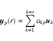 |
(4) |
| (5) |
![\begin{figure}
\par\includegraphics[width=15cm,clip]{7334fig02CMJN.eps} \end{figure}](/articles/aa/full/2007/21/aa7334-07/img47.gif) |
Figure 2: Reconstruction of SDSS/SEGUE spectra by projection onto synthetic principal components. In each row, the spectrum on the left is the original and the following show the reconstruction using increasing numbers of principal components. The residual spectrum (original minus reconstructed) is shown in the bottom of each panel. The quoted atmospheric parameters are taken from a preliminary version of the processing pipeline SSPP. |
| Open with DEXTER | |
![\begin{figure}
\par\includegraphics[width=15cm]{7334fig03CMJN.eps}\end{figure}](/articles/aa/full/2007/21/aa7334-07/img48.gif) |
Figure 3: As Fig. 2 but for principal components built from real spectra. |
| Open with DEXTER | |
If the number of spectra is smaller than the dimensionality of the data, i.e.,
if n < N, then the spectra span a subspace of dimensionality n. In this
case only n PCs are defined and a full reconstruction is achieved with
N=n. With ![]() ,
then using all PCs in the reconstruction means that
any spectrum - even one not used to form the PCs - can be
reconstructed exactly. With n < N this is no longer true. This is actually
the case with our synthetic data, where n=1816 and N=3818. This
potentially reduces the quality of any reconstruction, because some of the
data space is not spanned by the PCs.
,
then using all PCs in the reconstruction means that
any spectrum - even one not used to form the PCs - can be
reconstructed exactly. With n < N this is no longer true. This is actually
the case with our synthetic data, where n=1816 and N=3818. This
potentially reduces the quality of any reconstruction, because some of the
data space is not spanned by the PCs.
Reduced spectral reconstructions for five representative SDSS/SEGUE stars,
using different numbers of eigenvectors computed from the synthetic and real
spectra, are shown in Figs. 2 and 3 respectively. The
residual spectrum, defined as the difference between the original and the
reconstructed spectrum, is shown at the bottom
for each pattern
and each reconstruction. From inspection of these samples, one
can see how the PCA approach acts as an effective
filter to remove noise, recover missing and/or borderline features, and to
detect outliers in a spectrum that are reconstructed with large errors
(e.g., Storrie-Lombardi et al. 1995; Bailer-Jones et al. 1998).
However, here we also note that there is evidence that the Kurucz model
spectra we have adopted do not well describe SDSS/SEGUE spectra of cool
stars (
![]() K), especially when few PCs are retained in the
reconstruction. The residual spectrum of main sequence stars having
K), especially when few PCs are retained in the
reconstruction. The residual spectrum of main sequence stars having
![]() K and
K and
![]() K highlights difficulties in reproducing, with 5+5 and 25+25 PCs, the
K highlights difficulties in reproducing, with 5+5 and 25+25 PCs, the ![]() band at 5165
band at 5165 ![]() (see Fig. 2).
(see Fig. 2).
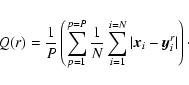
A useful measure of the reconstruction error over a set of P spectra is
In summary, a PCA compression retains those spectral features which are most common across the data set. It preferentially removes noise (and rare features), because they are statistically uncorrelated. Note that the atmospheric parameters are not used in defining the PCs.
Thus, considering the above, the choice of the optimal number of PCs to retain is a trade-off between retaining information versus reducing dimensionality and noise, and should be optimized in conjunction with the regression model. There exist more sophisticated methods of dimensionality reduction which could be used in the future, such as local and nonlinear variations on PCA (see Einbeck et al. (2007) for a review and astronomical application).
The restriction of an analysis to certain wavelength intervals via the
exclusion of (hopefully) unimportant ranges, is an alternative way to reduce
the dimensionality of the input space. This provides a way of directly
introducing domain information into the regression model. While this selection
is potentially difficult (and the number of permutations extremely large), we
show below that this approach is particularly effective for the estimation of
the surface gravity parameter, ![]() .
After considering a number of
alternatives, we chose to restrict the analysis on the wavelength ranges
3900-4400
.
After considering a number of
alternatives, we chose to restrict the analysis on the wavelength ranges
3900-4400 ![]() ,
4820-5000 Å, 5155-5350
,
4820-5000 Å, 5155-5350 ![]() ,
and 8500-8700
,
and 8500-8700 ![]() in
the spectra. These regions contain the most prominent hydrogen and metal
lines, including CaII K and H, the Balmer lines H
in
the spectra. These regions contain the most prominent hydrogen and metal
lines, including CaII K and H, the Balmer lines H![]() ,
H
,
H![]() ,
and
H
,
and
H![]() ,
the CH G-band, the Mg Ib triplet, and the CaII triplet.
,
the CH G-band, the Mg Ib triplet, and the CaII triplet.
In this section we report the results of the three types of models developed, SS, RR and SR (for a definition of these see Sect. 1).
For this analysis we adopt the sample of 1816 noise free synthetic spectra described in Sect. 2.2. This is randomly split into two equal-sized sets - one for model training, and one for model evaluation.
After a preliminary analysis with the full spectra, we decided to use a PCA
pre-processing of the data (Sect. 4.1). Principal components are
computed using the training set, then both sets are projected onto them to
yield the admixture coefficients, which are then the regression model inputs.
PCA is performed on the blue and red spectra separately, because this gave a
better reconstruction (which in turn reduced systematic offsets in the derived
parameters).
Table 1 shows typical parametrization errors for the three stellar
atmospheric parameters for different numbers of PCs retained in the
reconstruction; they all are very small and surprisingly lower for ![]() than for
than for
![]() .
We remark that, when increasing the number of PCs, the error is initially
determined predominantly by the amount of information present in the
reconstructed spectra, then by the limited ability of the non-linear
regression model to make full use of the available information.
These results, and the analysis of the reconstructed spectra, led us to select 25 (blue region) +25 (red region) PCs for the model.
.
We remark that, when increasing the number of PCs, the error is initially
determined predominantly by the amount of information present in the
reconstructed spectra, then by the limited ability of the non-linear
regression model to make full use of the available information.
These results, and the analysis of the reconstructed spectra, led us to select 25 (blue region) +25 (red region) PCs for the model.
![\begin{figure}
\par\resizebox{8.8cm}{!}
{\includegraphics[angle=-90,width=8.8cm]{7334fig04.ps}} \end{figure}](/articles/aa/full/2007/21/aa7334-07/img58.gif) |
Figure 4: PCA spectral reconstruction error, Q (defined in Eq. 6) on the evaluation data set for SR/RR/SS (solid/dashed/dotted lines, respectively) as a function of the number of eigenvectors, r, used for reconstruction. |
| Open with DEXTER | |
Table 1: Mean absolute errors on the evaluation set of 908 spectra in the SS model for different numbers of PCs retained in the reconstruction. (As PCA is done separately on the blue and red regions, the total number of inputs is twice the number of PCs.).
The above results were obtained with noise-free data, which is not very
realistic, so we also trained models where both the training and evaluation set
are degraded with Gaussian additive noise to signal-to-noise (SNR) levels of 10/1, 30/1, 50/1 and 100/1. Even at a SNR of 10/1, the errors are increased
by only 50 K in
![]() ,
0.02 dex in
,
0.02 dex in ![]() ,
and
0.03 dex in
,
and
0.03 dex in
![]() .
This modest deterioration is on account of the artifically good correspondence
between the training and evaluation set when using purely synthetic data;
the PCA noise filtering also appears to help. Note that whenever we
use synthetic spectra to define the PCs, we always use noise-free spectra
(also in Sect. 5.3).
.
This modest deterioration is on account of the artifically good correspondence
between the training and evaluation set when using purely synthetic data;
the PCA noise filtering also appears to help. Note that whenever we
use synthetic spectra to define the PCs, we always use noise-free spectra
(also in Sect. 5.3).
Following from our experience with the SS analysis, we build an RR regression
model to parametrize real spectra. The training and evaluation data sets are
taken from a set of 38 731 stars from 140 SDSS/SEGUE plates, in directions of
low reddening, which have had atmospheric parameters estimated by a
preliminary version of the SSPP. Both training and evaluation sets are drawn
at random (without replacement) with sizes 19 731 and 19 000 spectra
respectively. We use 2151 pixels in the blue spectrum between
3850-6000 ![]() and 1667 pixels in the red spectrum between
6500-9000
and 1667 pixels in the red spectrum between
6500-9000 ![]() .
A PCA compression reduces this to 25 (blue) +25 (red)
PCs, the PCs themselves formed only from the training set. This compresses the
data to 1.3% of its former size, resulting in more stable and faster
models. We use these data to predict
.
A PCA compression reduces this to 25 (blue) +25 (red)
PCs, the PCs themselves formed only from the training set. This compresses the
data to 1.3% of its former size, resulting in more stable and faster
models. We use these data to predict
![]() ,
,
![]() ,
and
,
and
![]() .
The standard deviations (essentially an estimate of their parameter ranges) of the input parameter
distributions are
.
The standard deviations (essentially an estimate of their parameter ranges) of the input parameter
distributions are
![]() K,
K,
![]() dex, and
dex, and
![]() dex,
respectively. These are on the order of the RMS errors which a random
classifier would achieve.
dex,
respectively. These are on the order of the RMS errors which a random
classifier would achieve.
![\begin{figure}
\par\includegraphics[angle=-90,width=15cm]{7334fig05.ps} \end{figure}](/articles/aa/full/2007/21/aa7334-07/img65.gif) |
Figure 5:
Atmospheric parameters estimation with
the RR model. We compare our estimated
|
| Open with DEXTER | |
In addition to this purely spectral model, we developed another model in which the four (de-reddened) photometric colours u-g, g-r, r-i, and i-z are added as four additional model inputs (they are not involved in the PCA).
Figure 5 compares our model estimates with those from the SSPP on the
evaluation set. Overall we see good consistency, especially for stars with
![]() K (
K (
![]() ). Above this effective
temperature we see that our models underestimate
). Above this effective
temperature we see that our models underestimate
![]() relative
to the SSPP. Our regression models are designed to smooth, i.e. interpolate,
data. Extrapolation of the model to estimate atmospheric parameters that are
not spanned by the training set is relatively unconstrained (and any model
would need to make additional assumptions). Furthermore, the accuracy of the
RR model is limited by the accuracy of the target atmospheric parameters used
in training, as well as their consistency across the parameter space. In this
case, the SSPP estimates are combinations from several estimation models, each
of which operates only over a limited parameter range. Thus, the transition we
see above 8000 K may indicate a temperature region where one of the SSPP
submodels is dominating the SSPP estimates, and this is not well-generalized
by our model. Of course, if we decided that we wanted to reproduce the SSPP
predictions for hot stars, we could do this simply by fitting a second-order
polynomial to our residuals to remove the systematic offset.
relative
to the SSPP. Our regression models are designed to smooth, i.e. interpolate,
data. Extrapolation of the model to estimate atmospheric parameters that are
not spanned by the training set is relatively unconstrained (and any model
would need to make additional assumptions). Furthermore, the accuracy of the
RR model is limited by the accuracy of the target atmospheric parameters used
in training, as well as their consistency across the parameter space. In this
case, the SSPP estimates are combinations from several estimation models, each
of which operates only over a limited parameter range. Thus, the transition we
see above 8000 K may indicate a temperature region where one of the SSPP
submodels is dominating the SSPP estimates, and this is not well-generalized
by our model. Of course, if we decided that we wanted to reproduce the SSPP
predictions for hot stars, we could do this simply by fitting a second-order
polynomial to our residuals to remove the systematic offset.
Table 2 quantifies the overall discrepacies for each parameter.
An error in
![]() of 0.0126 is an error of 2.9%, or 170 K at
6000 K. The last line in the table is the performance when we include
photometry. Adding photometry leads to significant improvement in all three
atmospheric parameters. This is not surprising for effective temperature, as
the photometric calibration of these bands is less complicated than the
spectral calibration.
A more accurate
of 0.0126 is an error of 2.9%, or 170 K at
6000 K. The last line in the table is the performance when we include
photometry. Adding photometry leads to significant improvement in all three
atmospheric parameters. This is not surprising for effective temperature, as
the photometric calibration of these bands is less complicated than the
spectral calibration.
A more accurate
![]() will permit more accurate
will permit more accurate ![]() and
and
![]() .
Thus, in directions where interstellar reddening is known to
be low, photometry should be used. The values listed in the table for a given
parameter are averaged over all values of the adopted atmospheric parameters.
Results for
gravity, metallicity, and effective temperature ranges
- dwarfs/giants, low/high metallicity, and cool/warm stars - are listed
in Table 5 and in Table 6.
.
Thus, in directions where interstellar reddening is known to
be low, photometry should be used. The values listed in the table for a given
parameter are averaged over all values of the adopted atmospheric parameters.
Results for
gravity, metallicity, and effective temperature ranges
- dwarfs/giants, low/high metallicity, and cool/warm stars - are listed
in Table 5 and in Table 6.
We have shown above that our regression models are capable of obtaining accurate and consistent estimates of atmospheric parameters when trained and tested on synthetic spectra (SS), and also when trained on real spectra with existing parametrizations and applied to another sample of real spectra (RR). We now develop the hybrid approach, SR, in which we train on synthetic spectra and use this model to determine atmospheric parameters for SDSS/SEGUE spectra directly. A very important aspect of this model is processing the synthetic and real data to look similar; inaccurate synthetic spectra (e.g. poor models or a poor flux calibration) will degrade performance and/or give rise to systematic errors.
Table 2: Mean absolute errors on the evaluation set of 19 000 spectra in the RR model (plotted in Fig. 5). The first line is for the full data set (training and evaluation data). The second and third are just for the evaluation sets. The third line is for a model which included the four photometric colours as additional model inputs (predictors).
Experience shows that it is advantageous to match the noise properties of
the synthetic training sample to that of the real sample. Essentially, noise
acts as a regularizer in the training phase and thus improves the overall
generalization performance of the models (e.g.; Odewahn et al. 2002; Snider et al. 2001),
in particular reducing systematics. For each of the 38 731 SDSS/SEGUE
stars in the evaluation set we use the SNR reported (for each pixel) in
the data array included in the FITS file (which was estimated by the reduction
pipeline). We assign a global SNR to the spectrum which is the median of all
flux bins over the wavelength range we retain (viz. 4000-5850 ![]() and
6500-8500
and
6500-8500 ![]() ). Figure 6 shows the distribution of these SNR
values. Based on this, we chose to develop two regression models, one
optimized for low SNR real spectra (
). Figure 6 shows the distribution of these SNR
values. Based on this, we chose to develop two regression models, one
optimized for low SNR real spectra (
![]() ,
13 487 stars) the other for
high SNR real spectra (
,
13 487 stars) the other for
high SNR real spectra (
![]() ,
25 244 stars). Experimentation showed that
this noise injection does indeed reduce systematics which are obtained when
using noise-free data for training.
,
25 244 stars). Experimentation showed that
this noise injection does indeed reduce systematics which are obtained when
using noise-free data for training.
![\begin{figure}
\par\resizebox{8.8cm}{!}
{\includegraphics[angle=-90,width=8.8cm]{7334fig06.ps}} \end{figure}](/articles/aa/full/2007/21/aa7334-07/img70.gif) |
Figure 6: Histogram of the SNR distribution for all 38 731 stars of the real sample. For each of them, the value for SNR has been estimated from the stellar spectrum. |
| Open with DEXTER | |
![\begin{figure}
\par\includegraphics[angle=-90,width=17cm]{7334fig07.ps} \end{figure}](/articles/aa/full/2007/21/aa7334-07/img71.gif) |
Figure 7:
Atmospheric parameters estimation with
the SR model. Comparison between our derived
|
| Open with DEXTER | |
We explored the application of dimensionality reduction with PCA, but found
that this led to rather large systematic errors in the parameters, in
particular in ![]() (up to 1.0 dex). We instead found that it is better
simply to select wavelength regions which are known to be the most sensitive
to surface gravity (e.g. 3900-4400
(up to 1.0 dex). We instead found that it is better
simply to select wavelength regions which are known to be the most sensitive
to surface gravity (e.g. 3900-4400 ![]() ,
4820-5000
,
4820-5000 ![]() ,
5155-5350
,
5155-5350 ![]() and 8500-8700
and 8500-8700 ![]() ). This is perhaps not unexpected, since
essentially all of the methods that are used by the SSPP to define the target
). This is perhaps not unexpected, since
essentially all of the methods that are used by the SSPP to define the target
![]() values use only these restricted wavelength ranges. This may also
indicate that the gravity signature in real stars outside of the wavelength
regions selected above behaves differently from the signature in the synthetic
spectra. Either way, the excluded regions show less sensitivity to
values use only these restricted wavelength ranges. This may also
indicate that the gravity signature in real stars outside of the wavelength
regions selected above behaves differently from the signature in the synthetic
spectra. Either way, the excluded regions show less sensitivity to ![]() ,
so for this parameter these regions do not add information, only
data that are uncorrelated with the parameter of interest (so are effectively
just noise). It is also possible, of course, that the PCA may be filtering out
subtle (weak) features which are strong predictors of
,
so for this parameter these regions do not add information, only
data that are uncorrelated with the parameter of interest (so are effectively
just noise). It is also possible, of course, that the PCA may be filtering out
subtle (weak) features which are strong predictors of ![]() .
.
Based on the above considerations, our final model uses PCA for estimating
![]() and
and
![]() and WRS for estimating
and WRS for estimating ![]() .
A separate
model is used for estimating each parameter (although the
.
A separate
model is used for estimating each parameter (although the
![]() model
also predicts the other two, the results of which are disregarded).
model
also predicts the other two, the results of which are disregarded).
Figure 7 compares our model atmospheric parameter estimates with those
from the preliminary SSPP for the 38 731 stars in the evaluation set. While
the overall consistency between the two models is reasonably good, we (again)
notice discrepancies at the extreme parameter values, in particular for
![]() .
This is sometimes an indication that the model has not been well
trained, i.e., it has not located a good local minimum of the error function
(it can never be shown that the global minimum has been found with anything
but an exhaustive search). However, there are inevitably problems with
spectral mismatch, in the sense that the synthetic spectra do not reproduce
all of the complexities of the spectra of real stars. The absence of several
molecular species in the linelists for the synthetic spectra may also be
contributing to this problem, especially for cooler stars where they are
expected to be more important.
For the determination of metallicity, we observe that our model
predicts lower metallicities for the lowest metallicity stars. This is probably
a consequence of the lack of synthetic samples between
.
This is sometimes an indication that the model has not been well
trained, i.e., it has not located a good local minimum of the error function
(it can never be shown that the global minimum has been found with anything
but an exhaustive search). However, there are inevitably problems with
spectral mismatch, in the sense that the synthetic spectra do not reproduce
all of the complexities of the spectra of real stars. The absence of several
molecular species in the linelists for the synthetic spectra may also be
contributing to this problem, especially for cooler stars where they are
expected to be more important.
For the determination of metallicity, we observe that our model
predicts lower metallicities for the lowest metallicity stars. This is probably
a consequence of the lack of synthetic samples between
![]() (see Fig. 1) in our current grid.
(see Fig. 1) in our current grid.
Table 3:
Mean absolute discrepancies (between our SR model and SSPP)
calculated on the evaluation set of 38 731 real spectra (see also
Fig. 7). Our models use PCA pre-processing for estimating
![]() and
and
![]() and WRS pre-processing for
estimating
and WRS pre-processing for
estimating ![]() ;
for the latter, PCA results are shown for
comparison. Separate models were applied for low and high SNR spectra
(the transition being at
;
for the latter, PCA results are shown for
comparison. Separate models were applied for low and high SNR spectra
(the transition being at
![]() ).
).
Table 3 shows the global results (averaged over all stars and
atmospheric parameters). It is interesting that the WRS pre-processing results
in little difference in the ![]() discrepancy for the low and high SNR
regimes. Results for
gravity, metallicity, and effective temperature ranges
- dwarfs/giants, low/high metallicity, and
cool/warm stars - are listed in Table 7 and in
Table 8, and visualized in Fig. 8. We note
that, in the estimation of
discrepancy for the low and high SNR
regimes. Results for
gravity, metallicity, and effective temperature ranges
- dwarfs/giants, low/high metallicity, and
cool/warm stars - are listed in Table 7 and in
Table 8, and visualized in Fig. 8. We note
that, in the estimation of ![]() ,
a systematic difference (our model
predictions lower than SSPP) occurs in the range
,
a systematic difference (our model
predictions lower than SSPP) occurs in the range
![]() -6700 K for
low-metallicity giants. Unfortunately we cannot include photometry in the SR models, because the
synthetic colours are not yet well-calibrated, and their zero points on the AB
system are still under discussion.
-6700 K for
low-metallicity giants. Unfortunately we cannot include photometry in the SR models, because the
synthetic colours are not yet well-calibrated, and their zero points on the AB
system are still under discussion.
![\begin{figure}
\par\includegraphics[angle=-90,width=17cm]{7334fig08.ps} \end{figure}](/articles/aa/full/2007/21/aa7334-07/img74.gif) |
Figure 8:
More detailed visualization of the SR model discrepancies
(Fig. 7). The diamonds joined by lines show mean absolute
residual (solid lines) and mean residual (dashed lines) for low
metallicity (
|
| Open with DEXTER | |
The RR and SR models developed above both appear to give reasonable
predictions, as measured by their mean accuracies with respect to the SSPP
predictions -
![]() with residual of
0.013/0.014 (
with residual of
0.013/0.014 (![]() 170 K),
170 K), ![]() with a residual of 0.36/0.45 dex and
with a residual of 0.36/0.45 dex and
![]() with a
residual of 0.19/0.26 dex for RR/SR respectively.
with a
residual of 0.19/0.26 dex for RR/SR respectively.
The global discrepancies are larger with SR for ![]() and
and
![]() ,
but this is not surprising because it is entirely independent of the SSPP
parameter estimates. While the synthetic spectra place a limit on the
performance of the SR model, this is true of any parametrization
model. Physical parameters can only be derived using physical models; none can
be measured "directly''. The advantage of the SR approach is that it only
uses one set in the parametrizations, it can easily be retrained using new
synthetic spectra, and it provides a quick, general model which operates over
the entire parameter range. In effect, the work in getting good predictions is
taken out of the machine learning model and moved to the definition of the
templates and the pre-processing.
,
but this is not surprising because it is entirely independent of the SSPP
parameter estimates. While the synthetic spectra place a limit on the
performance of the SR model, this is true of any parametrization
model. Physical parameters can only be derived using physical models; none can
be measured "directly''. The advantage of the SR approach is that it only
uses one set in the parametrizations, it can easily be retrained using new
synthetic spectra, and it provides a quick, general model which operates over
the entire parameter range. In effect, the work in getting good predictions is
taken out of the machine learning model and moved to the definition of the
templates and the pre-processing.
We find that PCA delivers more accurate atmospheric parameters when the
training data are the actual SDSS spectra with previously estimated
parameters, whereas WRS appears superior for the estimation of ![]() templates, especially from lower SNR spectra.
templates, especially from lower SNR spectra.
![\begin{figure}
\par\includegraphics[angle=-90,width=17cm]{7334fig09.ps} \end{figure}](/articles/aa/full/2007/21/aa7334-07/img76.gif) |
Figure 9: Comparison between SR and RR estimations on the 19 000 real spectra in common in their evaluation sets. The line shows the perfect correlation and the bottom panels the distributions of residuals. |
| Open with DEXTER | |
From the subsample of 19 000 stars used as the evaluation set in RR we
compare the SR predictions with the RR predictions (see Fig. 9). The
mean absolute differences are on the order of 0.010 in
![]() (150 K), 0.35 dex in
(150 K), 0.35 dex in ![]() ,
and 0.22 dex in
,
and 0.22 dex in
![]() .
.
Comparison of theoretical isochrones with data from clusters offers an
excellent opportunity to test the present model predictions. In particular,
we can use them to assess the calibration of the parameter determinations.
Here we focus our discussion on the globular cluster
![]() ,
but we have
also analysed the globular clusters
,
but we have
also analysed the globular clusters
![]() and
and ![]() and the open
cluster
and the open
cluster
![]() ,
all observed by SDSS/SEGUE. We select likely members,
then estimate their atmospheric parameters, and overplot these on a set of
isochrones fixed at literature values for the cluster distance modulus, age,
and metallicity. If these values (and the isochrones themselves) are correct,
discrepancies between our estimates and the isochrones would indicate problems
in the calibrations of the atmospheric parameters (e.g. of the synthetic
spectra on which the regression models are based). We note that Lee et al. (2007)
have looked more carefully at the three globular clusters, and make an
independent target selection based also on stellar densities, from which they
derive mean metallicities and radial velocities for the clusters.
,
all observed by SDSS/SEGUE. We select likely members,
then estimate their atmospheric parameters, and overplot these on a set of
isochrones fixed at literature values for the cluster distance modulus, age,
and metallicity. If these values (and the isochrones themselves) are correct,
discrepancies between our estimates and the isochrones would indicate problems
in the calibrations of the atmospheric parameters (e.g. of the synthetic
spectra on which the regression models are based). We note that Lee et al. (2007)
have looked more carefully at the three globular clusters, and make an
independent target selection based also on stellar densities, from which they
derive mean metallicities and radial velocities for the clusters.
The globular cluster
![]() is located in the sky at
is located in the sky at
![]() ,
,
![]() (Harris 1996), and has been extensively studied in the past (e.g., Binney & Merrifield 1998; Sandage 1970). SDSS/SEGUE plates 1960 and 1962 include observations of
its members. Figure 10 shows the distribution of the 526 stars with
available SDSS/SEGUE spectroscopy and ugriz photometry. The central regions
of the clusters are not generally available for spectroscopic observation, due
to fibre placement restrictions in the SDSS spectrographs. This must be borne
in mind when interpreting the results we describe below.
(Harris 1996), and has been extensively studied in the past (e.g., Binney & Merrifield 1998; Sandage 1970). SDSS/SEGUE plates 1960 and 1962 include observations of
its members. Figure 10 shows the distribution of the 526 stars with
available SDSS/SEGUE spectroscopy and ugriz photometry. The central regions
of the clusters are not generally available for spectroscopic observation, due
to fibre placement restrictions in the SDSS spectrographs. This must be borne
in mind when interpreting the results we describe below.
Based on position, we initially select 133 candidate members in the region
![]() and
and
![]() ,
as represented by the box shown in Fig. 10.
,
as represented by the box shown in Fig. 10.
The distribution of the atmospheric parameters
![]() versus
versus ![]() of this sample, using both the RR and SR models, is shown in
Fig. 11. The stars clearly fall into two groups, due to false
cluster members which we can plausibly take to be stars projected in front of
the cluster from the Galactic field (generally at higher metallicity), and
stars from the globular cluster itself (lower metallicity). It is also
obvious that, given the apparent magnitude limits of SDSS/SEGUE, we would not
expect to see higher-gravity main sequence stars that are true cluster members.
of this sample, using both the RR and SR models, is shown in
Fig. 11. The stars clearly fall into two groups, due to false
cluster members which we can plausibly take to be stars projected in front of
the cluster from the Galactic field (generally at higher metallicity), and
stars from the globular cluster itself (lower metallicity). It is also
obvious that, given the apparent magnitude limits of SDSS/SEGUE, we would not
expect to see higher-gravity main sequence stars that are true cluster members.
To obtain a more clean sample of likely cluster members, we select from the observed sample using published estimates of radial velocities and metallicities for the cluster (see Table 4).
We first select based on radial velocity; specifically, we retain as
candidates only those stars with
![]() .
This cut preferentially
excludes metal-rich main sequence stars, and results in a remaining sample that
contains 40 candidates with
.
This cut preferentially
excludes metal-rich main sequence stars, and results in a remaining sample that
contains 40 candidates with
![]() out of a total of 42.
out of a total of 42.
We define a second sample, now of main sequence stars; namely, the 8 or 7 stars
(for RR/SR respectively) having metal abundance
![]() and
and
![]() ,
without any radial velocity selection.
Using the absolute magnitude determination for
late-type dwarfs as a function of SDSS photometry (Bilir et al. 2005)
,
without any radial velocity selection.
Using the absolute magnitude determination for
late-type dwarfs as a function of SDSS photometry (Bilir et al. 2005)
| Mg=5.791(g-r)+1.242(r-i)+1.412 | (7) |
The complete sample of
![]() cluster members has 46 (RR)/ 45 (SR)
stars. The entire radial velocity selected sample is shown in
Fig.11 with filled circles, while the metal-poor main sequence
stars we suspect are cluster members are shown with asterisks.
cluster members has 46 (RR)/ 45 (SR)
stars. The entire radial velocity selected sample is shown in
Fig.11 with filled circles, while the metal-poor main sequence
stars we suspect are cluster members are shown with asterisks.
![]() has been previously analysed during the course of the development
of the SSPP. Our initial sample (of 133 stars) includes 26 of the 35
candidates. Of these, 7 stars which have been rejected on the grounds of their
apparently discrepant estimated abundance, or lack of an estimate at all, are
marked with a plus sign. The 19 stars confirmed as likely members are also
identified as part of our candidate members; we highlight these as
grey dots in Fig. 11.
Inspection of this figure shows the
has been previously analysed during the course of the development
of the SSPP. Our initial sample (of 133 stars) includes 26 of the 35
candidates. Of these, 7 stars which have been rejected on the grounds of their
apparently discrepant estimated abundance, or lack of an estimate at all, are
marked with a plus sign. The 19 stars confirmed as likely members are also
identified as part of our candidate members; we highlight these as
grey dots in Fig. 11.
Inspection of this figure shows the
![]() members as a clump of stars,
albeit one which is more clumped in the RR predictions of the atmospheric
parameters than in the SR predictions of the atmospheric parameters.
members as a clump of stars,
albeit one which is more clumped in the RR predictions of the atmospheric
parameters than in the SR predictions of the atmospheric parameters.
From the sample of cluster members with consistent metallicities and radial
velocities we obtain a mean metallicity of
![]() dex (RR)/
dex (RR)/
![]() dex (SR). Using just the giants in this sample (i.e., excluding the metal-poor main
sequence stars) we obtain
dex (SR). Using just the giants in this sample (i.e., excluding the metal-poor main
sequence stars) we obtain
![]() dex (RR)/
dex (RR)/
![]() dex (SR). These values are in good agreement with previous determinations in the literature (see Table 4).
dex (SR). These values are in good agreement with previous determinations in the literature (see Table 4).
![\begin{figure}
\par\includegraphics[angle=-90,width=7.5cm,clip]{aa7334fig10NEW.ps}\end{figure}](/articles/aa/full/2007/21/aa7334-07/img88.gif) |
Figure 10:
Distribution on the sky of the 526 stars present from SDSS/SEGUE plates 1960 and 1962. The box defines the selection criteria (
|
| Open with DEXTER | |
![\begin{figure}
\par\includegraphics[angle=0,width=7.5cm,clip]{7334fig11.ps} \end{figure}](/articles/aa/full/2007/21/aa7334-07/img89.gif) |
Figure 11:
Distribution of
|
| Open with DEXTER | |
We now compare our atmospheric parameter estimates with theoretical SDSS
isochrones from Girardi et al. (2004). We adopt an age of 13.2 Gyr, a metallicity
![]() dex, and a distance modulus of 14.93 (e.g., Binney & Merrifield 1998; Sandage 1970).
dex, and a distance modulus of 14.93 (e.g., Binney & Merrifield 1998; Sandage 1970).
Figure 12 shows the colour-magnitude and effective
temperature-gravity diagrams for the likely
![]() members overplotted
with the theoretical isochrones. These isochrones bracket the candidates
reasonably well in the colour-magnitude diagram, but the distribution
in the atmospheric parameter plane shows systematic offsets, in particular for
the RR model estimates. A zero-point offset in either the gravity or
temperature parameterizations (or in the isochrones) would improve the
coincidence. On the other hand, the RR model clearly yields a tighter
distribution in the atmospheric parameters.
Thus, if we believe the isochrones, then we can conclude that the RR model
obtains more precise parameter estimates, while the SR model obtains
more accurate ones. In fact, if we would attribute the offset due
entirely to gravity, we would have to apply corrections of about 0.60 dex (RR)
or 0.25 dex (SR) to our estimates in order to obtain coincidence with their
predicted location in the effective temperature-gravity planes.
members overplotted
with the theoretical isochrones. These isochrones bracket the candidates
reasonably well in the colour-magnitude diagram, but the distribution
in the atmospheric parameter plane shows systematic offsets, in particular for
the RR model estimates. A zero-point offset in either the gravity or
temperature parameterizations (or in the isochrones) would improve the
coincidence. On the other hand, the RR model clearly yields a tighter
distribution in the atmospheric parameters.
Thus, if we believe the isochrones, then we can conclude that the RR model
obtains more precise parameter estimates, while the SR model obtains
more accurate ones. In fact, if we would attribute the offset due
entirely to gravity, we would have to apply corrections of about 0.60 dex (RR)
or 0.25 dex (SR) to our estimates in order to obtain coincidence with their
predicted location in the effective temperature-gravity planes.
We carried out the same analysis for three additional clusters which have also
been extensively studied in the past, and so have reasonably consistent
determinations of metallicity, age, and distance in the literature (see
Table 4). Candidate stars from the globular clusters
![]() (e.g., Binney & Merrifield 1998; Harris 1996; Shetrone 1994; Lupton et al. 1987; Sandage 1970) appear on SEGUE plates
2174, 2185, and 2255; from the globular cluster
(e.g., Binney & Merrifield 1998; Harris 1996; Shetrone 1994; Lupton et al. 1987; Sandage 1970) appear on SEGUE plates
2174, 2185, and 2255; from the globular cluster ![]() (e.g.,
Harris 1996; Lázaro et al. 2006) on SEGUE plate 1961; and from the open cluster
(e.g.,
Harris 1996; Lázaro et al. 2006) on SEGUE plate 1961; and from the open cluster
![]() (e.g.; McClure et al. 1974; Tianxing 1987; Smith 1987) on SEGUE plates 2078and 2079. For each of these, we select likely members following the same
procedures as for the
(e.g.; McClure et al. 1974; Tianxing 1987; Smith 1987) on SEGUE plates 2078and 2079. For each of these, we select likely members following the same
procedures as for the
![]() analysis (Sect. 6.1) and
compare them with isochrones with parameters based on previous analyses.
analysis (Sect. 6.1) and
compare them with isochrones with parameters based on previous analyses.
![\begin{figure}
\par\resizebox{18cm}{!}{\includegraphics[angle=-90,width=17cm]
{7334fig12.ps}} \end{figure}](/articles/aa/full/2007/21/aa7334-07/img91.gif) |
Figure 12:
The left panel shows the colour-magnitude diagram for M 15, and
the two other panels the distribution of atmospheric parameters
|
| Open with DEXTER | |
![\begin{figure}
\par\includegraphics[angle=-90,width=16cm]{7334fig13.ps} \end{figure}](/articles/aa/full/2007/21/aa7334-07/img92.gif) |
Figure 13:
As Fig. 12. Top:
|
| Open with DEXTER | |
Table 4: Globular/Open Clusters, literature values. The selection constraints applied for identification of likely members are labeled with *.
Table 5:
RR: partial results. We list the mean ![]() and the
corresponding standard deviation
and the
corresponding standard deviation ![]() of the difference
Committee-SSPP for each of the different stellar types and parameter
ranges.
of the difference
Committee-SSPP for each of the different stellar types and parameter
ranges.
Figure 13 shows the distribution of the atmospheric parameters for
expected members of each cluster in the colour-magnitude and in the
![]() plane, overplotted with the theoretical
isochrones selected to best match each cluster's properties. Inspection of
these distributions confirms our previous conclusions for the case of
plane, overplotted with the theoretical
isochrones selected to best match each cluster's properties. Inspection of
these distributions confirms our previous conclusions for the case of
![]() - (1) there exists a systematic offset in effective temperature
and/or surface gravity between the estimated parameters and those expected
from the theoretical isochrones, and (2) the RR model provides more precise
atmospheric parameter estimates, while the SR model provides more accurate
ones.
- (1) there exists a systematic offset in effective temperature
and/or surface gravity between the estimated parameters and those expected
from the theoretical isochrones, and (2) the RR model provides more precise
atmospheric parameter estimates, while the SR model provides more accurate
ones.
We are limited by the small number of likely cluster members in some cases,
especially for ![]() ,
which (so far) appears on only one SEGUE plate.
However, it seems that this evidence is more clearly visible in the globular
clusters which, as for
,
which (so far) appears on only one SEGUE plate.
However, it seems that this evidence is more clearly visible in the globular
clusters which, as for
![]() ,
are old and metal poor.
In the atmospheric parameter plane, the distribution for the open
cluster
,
are old and metal poor.
In the atmospheric parameter plane, the distribution for the open
cluster
![]() from the SR model looks a bit confusing. It is
plausible that this cluster is too metal-rich
to obtain good atmospheric parameter estimates, as the expected parameters are
at the extreme of the regions covered by the synthetic grid used for training.
Larger uncertainties are certainly present in this range of metallicity
(see Tables 7, 8). These limitations are
under study at the moment.
from the SR model looks a bit confusing. It is
plausible that this cluster is too metal-rich
to obtain good atmospheric parameter estimates, as the expected parameters are
at the extreme of the regions covered by the synthetic grid used for training.
Larger uncertainties are certainly present in this range of metallicity
(see Tables 7, 8). These limitations are
under study at the moment.
We have developed models to estimate the three primary stellar atmospheric
parameters (
![]() ,
,
![]() ,
and
,
and
![]() )
from
SDSS/SEGUE spectra. These models produce self-consistent parameter
estimates and can be implemented into an automated data processing
pipeline. Our models rely on an initial configuration (or "training'')
phase, which for one of the models (RR) uses pre-classified observed data,
for the other (SR) synthetic spectra selected by the user. Both are
flexible, in that new models can easily be introduced by changing the set
of training templates.
)
from
SDSS/SEGUE spectra. These models produce self-consistent parameter
estimates and can be implemented into an automated data processing
pipeline. Our models rely on an initial configuration (or "training'')
phase, which for one of the models (RR) uses pre-classified observed data,
for the other (SR) synthetic spectra selected by the user. Both are
flexible, in that new models can easily be introduced by changing the set
of training templates.
Both models are nonlinear, regularized regression models. The RR model uses an initial PCA compression of the data to reduce the dimensionality (from 3818 to 50), thus producing a more robust (and precise) parametrizer (which reduces the dimensionality further to 3, i.e., the three atmospheric parameters). They are also rapid, requiring of the order of one millisecond per star on a single, modest CPU.
The RR model has the advantage that exactly the same type of data are used in the training and application phases, thus eliminating the issue of discrepancies in the flux calibration or cosmic variance of the two samples. Of course, this requires an independent estimation method ("basis parameterizer'') to parametrize the training templates (which itself must use synthetic models at some level). Our regression model then automates and - more importantly - generalizes this basis parameterizer. Indeed, the basis parameterizer may even comprise multiple algorithms, perhaps operating over different parameters ranges or used in a voting system to estimate atmospheric parameters. This is true in the present case, where the basis parameterizer comes from a preliminary version of the SDSS/SEGUE Spectroscopic Parameter Pipeline (SSPP; Beers et al. 2006; Lee et al. 2007).
Table 6:
RR: partial results. We list the mean ![]() and the
corresponding standard deviation
and the
corresponding standard deviation ![]() of the difference
Committee-SSPP for each of the different stellar temperatures and metallicity
ranges.
of the difference
Committee-SSPP for each of the different stellar temperatures and metallicity
ranges.
Table 7:
SR: partial results. We list the mean ![]() and the
corresponding standard deviation
and the
corresponding standard deviation ![]() of the difference
Committee-SSPP for each of the different stellar types and parameter
ranges.
of the difference
Committee-SSPP for each of the different stellar types and parameter
ranges.
In contrast, our SR model is trained directly on synthetic spectra,
dispensing with the need for a basis parameterizer. For best results these
training data should have noise properties similar to the observed data
(which improves the regularization). We therefore implemented different models
for different SNR ranges. PCA is again used for data compression, except
for the surface gravity parameter ![]() ,
where better results were obtained
using a subset of spectral features known to be most sensitive to this
parameter.
,
where better results were obtained
using a subset of spectral features known to be most sensitive to this
parameter.
For each atmospheric parameter, the accuracy of our predictions with respect to
previous estimates (SSPP) are
![]() to 170/170 K,
to 170/170 K, ![]() to
0.36/0.45 dex and
to
0.36/0.45 dex and
![]() to 0.19/0.26 dex for methods RR and SR
respectively. Consistency between the two approaches is on order of 150 K
in
to 0.19/0.26 dex for methods RR and SR
respectively. Consistency between the two approaches is on order of 150 K
in
![]() ,
0.35 dex in
,
0.35 dex in ![]() ,
and 0.22 dex in
,
and 0.22 dex in
![]() .
Some discrepancies are probably due to the different Kurucz models
adopted in our SR model and in some of the methods employed in the SSPP.
.
Some discrepancies are probably due to the different Kurucz models
adopted in our SR model and in some of the methods employed in the SSPP.
As a test of our model predictions, we estimated atmospheric parameters for globular/open cluster members and compared these to theoretical isochrones. We found that RR gives more precise parameter estimates (stars show smaller scatter) whereas SR gives more accurate ones (stars show smaller offset, or bias). We can use this information to improve the parameter calibration of the basis parametrizers or the pre-processing of the synthetic spectra. We have also used our models to estimate atmospheric parameters for 89 600 SEGUE and 194 172 SDSS (DR-5) stellar spectra, which are being used for further scientific investigations.
We found that the inclusion of the four SDSS photometric colours improves the precision of parameter estimation significantly, but this will only work for zero (or very low) extinction regions. In principle, our models can be extended to predict extinction (by inclusion of its variance in the training set), allowing us to then use both photometry and spectroscopy to predict atmospheric parameters along significantly reddened lines of sight.
Table 8:
SR: Partial results. We list the mean ![]() and the
corresponding standard deviation
and the
corresponding standard deviation ![]() of the difference
Committee-SSPP for each of the different stellar temperatures and metallicity
ranges.
of the difference
Committee-SSPP for each of the different stellar temperatures and metallicity
ranges.
Our RR model has already been successfully integrated into the SSPP. The
SR will undergo further refinement with improved synthetic spectra. In
particular, models with more molecules included in the linelists
will improve the representation of cool stars. An extension to hotter stars
will make the model more widely applicable (at present such stars can be
filtered out via the PCA reconsuction error). Looking further ahead, the SR
approach will form the basis for atmospheric parameter estimation from the
very low resolution spectrophotometry (![]() -40) to be obtained with
Gaia (albeit using a more sophisticated and knowledge-based approach to
regression, which also includes the accurate parallaxes and high-precision
photometry from Gaia).
Our pattern recognition approach is probably indispensable in such an
application, because the low resolution and spectral purity of the
spectrophotometry prevent the definition of traditional indices.
-40) to be obtained with
Gaia (albeit using a more sophisticated and knowledge-based approach to
regression, which also includes the accurate parallaxes and high-precision
photometry from Gaia).
Our pattern recognition approach is probably indispensable in such an
application, because the low resolution and spectral purity of the
spectrophotometry prevent the definition of traditional indices.
Acknowledgements
This work was partly funded by a DFG Emmy-Noether Nachwuchsgruppe grant to C.A.L. Bailer-Jones. Y.S. Lee, T.C. Beers, and T. Sivarani acknowledge partial support for this work from grant AST 04-06784, as well as from grant PHY 02-16783: Physics Frontiers Center/Joint Institute for Nuclear Astrophysics (JINA), both awarded by the U.S. National Science Foundation.We wish to thank the referee, Norbert Christlieb, for a careful reading of this manuscript and for his useful remarks.
Funding for the SDSS and SDSS-II has been provided by the Alfred P. Sloan Foundation, the Participating Institutions, the National Science Foundation, the U.S. Department of Energy, the National Aeronautics and Space Administration, the Japanese Monbukagakusho, the Max Planck Society, and the Higher Education Funding Council for England. The SDSS Web Site is http://www.sdss.org/.
The SDSS is managed by the Astrophysical Research Consortium for the Participating Institutions. The Participating Institutions are the American Museum of Natural History, Astrophysical Institute Potsdam, University of Basel, University of Cambridge, Case Western Reserve University, University of Chicago, Drexel University, Fermilab, the Institute for Advanced Study, the Japan Participation Group, Johns Hopkins University, the Joint Institute for Nuclear Astrophysics, the Kavli Institute for Particle Astrophysics and Cosmology, the Korean Scientist Group, the Chinese Academy of Sciences (LAMOST), Los Alamos National Laboratory, the Max-Planck-Institute for Astronomy (MPIA), the Max-Planck-Institute for Astrophysics (MPA), New Mexico State University, Ohio State University, University of Pittsburgh, University of Portsmouth, Princeton University, the United States Naval Observatory, and the University of Washington.