A&A 467, 1313-1344 (2007)
DOI: 10.1051/0004-6361:20065258
J. F. Macías-Pérez1 - G. Lagache2 -
B. Maffei3 - K. Ganga4 -
A. Bourrachot5 - P. Ade3 -
A. Amblard6 - R. Ansari5 -
E. Aubourg4,7 - J. Aumont1 -
S. Bargot5 - J. Bartlett4 -
A. Benoît8 - J.-Ph. Bernard9 -
R. Bhatia10 - A. Blanchard11 -
J. J. Bock12,13 -
A. Boscaleri14 -
F. R. Bouchet15 -
P. Camus8 -
J.-F. Cardoso16 -
F. Couchot5 -
P. de Bernardis17 -
J. Delabrouille4 -
F.-X. Désert18 -
O. Doré19,2,20 -
M. Douspis2,11 -
L. Dumoulin21 -
X. Dupac10 -
Ph. Filliatre1,22 -
P. Fosalba23,2 -
F. Gannaway3 -
B. Gautier8 -
M. Giard9 -
Y. Giraud-Héraud4 -
R. Gispert2,![]() ,
,![]() - L. Guglielmi4 -
J.-Ch. Hamilton24 -
S. Hanany25 - S. Henrot-Versillé5 -
V. Hristov12 - J. Kaplan 4 - J.-M. Lamarre26 - A. E. Lange12 - K. Madet8 - Ch. Magneville4,7 - D. P. Marrone25 -
S. Masi 17 - F. Mayet 1 - J. A. Murphy27 -
F. Naraghi1 - F. Nati17 -
G. Patanchon28 - O. Perdereau5 -
G. Perrin1 - S. Plaszczynski5 -
M. Piat4 - N. Ponthieu2 -
S. Prunet15 - J.-L. Puget2 -
C. Renault1 - C. Rosset5 - D. Santos1 - A. Starobinsky29 - I. Strukov30 - R. V. Sudiwala3 - R. Teyssier15 - M. Tristram5,1 - C. Tucker3 - J.-Ch. Vanel4 - D. Vibert15 - E. Wakui3 - D. Yvon7
- L. Guglielmi4 -
J.-Ch. Hamilton24 -
S. Hanany25 - S. Henrot-Versillé5 -
V. Hristov12 - J. Kaplan 4 - J.-M. Lamarre26 - A. E. Lange12 - K. Madet8 - Ch. Magneville4,7 - D. P. Marrone25 -
S. Masi 17 - F. Mayet 1 - J. A. Murphy27 -
F. Naraghi1 - F. Nati17 -
G. Patanchon28 - O. Perdereau5 -
G. Perrin1 - S. Plaszczynski5 -
M. Piat4 - N. Ponthieu2 -
S. Prunet15 - J.-L. Puget2 -
C. Renault1 - C. Rosset5 - D. Santos1 - A. Starobinsky29 - I. Strukov30 - R. V. Sudiwala3 - R. Teyssier15 - M. Tristram5,1 - C. Tucker3 - J.-Ch. Vanel4 - D. Vibert15 - E. Wakui3 - D. Yvon7
1 -
LPSC, Université Joseph Fourier Grenoble I, CNRS/IN2P3, Institut National Polytechnique de Grenoble, 53 Avenue des Martyrs, 38026 Grenoble Cedex, France
2 -
Institut d'Astrophysique Spatiale, Bât. 121, Université Paris XI, 91405 Orsay Cedex, France
3 -
Cardiff University, Physics Department, PO Box 913, 5 The Parade, Cardiff, CF24 3YB, UK
4 -
APC, Collège de France, 11 pl. M. Berthelot, 75231 Paris Cedex 5, France
5 -
Laboratoire de l'Accélérateur Linéaire, BP 34, Campus Orsay, 91898 Orsay Cedex, France
6 -
University of California, Berkeley, Dept. of Astronomy, 601 Campbell Hall, Berkeley, CA 94720-3411, USA
7 -
CEA-CE Saclay, DAPNIA, Service de Physique des Particules, Bât. 141, 91191 Gif-sur-Yvette Cedex, France
8 -
Centre de Recherche sur les Très Basses Températures, BP 166, 38042 Grenoble Cedex 9, France
9 -
Centre d'Étude Spatiale des Rayonnements, BP 4346, 31028 Toulouse Cedex 4, France
10 -
ESTEC, Noordwijk, The Netherlands
11 -
Laboratoire d'Astrophysique de Tarbes Toulouse, 14 Avenue E. Belin, 31400 Toulouse, France
12 -
California Institute of Technology, 105-24 Caltech, 1201 East California Blvd, Pasadena CA 91125, USA
13 -
Jet Propulsion Laboratory, 4800 Oak Grove Drive, Pasadena, California 91109, USA
14 - IROE-CNR, Firenze, Italy
15 - Institut d'Astrophysique de Paris, 98bis, Boulevard Arago, 75014 Paris, France
16 - CNRS-ENST 46, rue Barrault, 75634 Paris, France
17 - Gruppo di Cosmologia Sperimentale, Dipart. di Fisica, Univ. La
Sapienza, P. A. Moro 2, 00185 Roma, Italy
18 - Laboratoire d'Astrophysique, Obs. de Grenoble, BP 53, 38041 Grenoble Cedex 9, France
19 - Dpt of Astrophysical Sciences, Princeton University, Princeton, NJ08544 USA
20 - CITA, University of Toronto, 60 St George Street, Toronto, ON M5S 3H8, Canada
21 - CSNSM-IN2P3, Bât. 108, 91405 Orsay Campus, France
22 - CEA-CE Saclay, DAPNIA, Service d'Astrophysique, Bât. 709,
91191 Gif-sur-Yvette Cedex, France
23 - Instituto de Ciencias del Espacio (IEEC/CSIC), Facultad de Ciencias,
Campus UAB, 08193 Cerdanyola, Spain
24 - LPNHE, Universités Paris VI et Paris VII, 4 place Jussieu, Tour 33, 75252 Paris Cedex 05, France
25 - School of Physics and Astronomy, 116 Church St. S.E., University of Minnesota, Minneapolis MN 55455, USA
26 - LERMA, Observatoire de Paris, 61 Av. de l'Observatoire, 75014 Paris, France
27 - Experimental Physics, National University of Ireland, Maynooth, Ireland
28 - Department of Physics & Astronomy, University of British Columbia, Vancouver, Canada
29 - Landau Institute for Theoretical Physics, 119334 Moscow, Russia
30 - Space Research Institute, Profsoyuznaya St. 84/32, Moscow, Russia
Received 23 March 2006 / Accepted 10 January 2007
Abstract
Aims. Archeops is a balloon-borne experiment inspired by the Planck satellite and its high frequency instrument (HFI). It is designed to measure the cosmic microwave background (CMB) temperature anisotropies at high angular resolution (![]() 12 arcmin) over a large fraction of the sky (around 30%) at 143, 217, 353, and 545 GHz. The Archeops 353 GHz channel consists of three pairs of polarized sensitive bolometers designed to detect the polarized diffuse emission of Galactic dust.
12 arcmin) over a large fraction of the sky (around 30%) at 143, 217, 353, and 545 GHz. The Archeops 353 GHz channel consists of three pairs of polarized sensitive bolometers designed to detect the polarized diffuse emission of Galactic dust.
Methods. In this paper we present an update of the instrumental setup, as well as the flight performance for the last Archeops flight campaign (February 2002 from Kiruna, Sweden). We also describe the processing and analysis of the Archeops time-ordered data for that campaign, which led to measurement of the CMB anisotropy power spectrum in the multipole range
![]() and to the first measurements of both the polarized emission of dust at large angular scales and its power spectra in the multipole range
and to the first measurements of both the polarized emission of dust at large angular scales and its power spectra in the multipole range
![]()
Results. We present maps covering approximately 30% of the sky. These maps contain Galactic emission, including the Galactic plane, in the four Archeops channels at 143, 217, 353, and 545 GHz and CMB anisotropies at 143 and 217 GHz. These are one of the first sub-degree-resolution maps in the millimeter and submillimeter ranges of the large angular-scale diffuse Galactic dust emission and CMB temperature anisotropies, respectively.
Key words: methods: data analysis - cosmic microwave background
The measurement of the cosmic microwave background (CMB) anisotropies
in temperature and polarization is a fundamental test of our concepts of modern
cosmology and of the physics of the early Universe. Since the first detection
of CMB anisotropies by the COBE satellite in 1992 (Smoot et al. 1992), a
large number of ground-based and balloon-borne experiments, such as DASI
(Halverson et al. 2002), CBI (Mason et al. 2003), VSA (Dickinson et al. 2004), BOOMERanG
(Netterfield et al. 2002) and Maxima (Hanany et al. 2000), have measured the CMB
angular power spectra from a few-degrees down to sub-degree scales.
However, simultaneous observation of very large and small angular
scales have proved to be particularly difficult, as it requires both
large sky coverage and high angular resolution. This was first
achieved by this experiment, Archeops (Benoît et al. 2003a; Tristram et al. 2005b),
which measured the CMB power spectrum in the multipole range
![]() .
Since, the WMAP satellite mission (Bennett et al. 2003)
has detected the CMB anisotropies, both in temperature and polarization.
.
Since, the WMAP satellite mission (Bennett et al. 2003)
has detected the CMB anisotropies, both in temperature and polarization.
Archeops, described in detail in Benoît et al. (2002), is a balloon-borne experiment designed as a testbed for many of the technologies to be used on the high frequency instrument (HFI) of the Planck satellite. Its telescope and focal plane optics are widely inspired by the Planck design. Implementation of the measurement chains - cryogenics, optics, bolometers, readout electronics - validated the innovative design. Moreover, the data processing has been a learning process for members of the HFI team.
Archeops performs circular scans on the sky with its optical axis tilted 41 degrees with respect to the horizon, spinning the gondola at 2 rpm. This scanning, combined with the rotation of the Earth, leads to 30% sky coverage in about 12 h of flight. With a rotating gondola, the Sun above the horizon produces a dominant parasitic signal. One way to avoid this, while conserving integration time, is by having a long duration (Arctic) night-time balloon flight.
The Archeops payload was successfully launched three times:
first, from Trapani, Italy, in July 1999 (Benoît et al. 2002) for a 4 h test flight; second, from the Swedish Esrange station in January
2001 for a 12-h flight (near Kiruna, Sweden, at 68 deg. latitude
North, just above the Arctic circle. Esrange is operated by the French
Centre National d'Etudes Spatiales, CNES, and the Swedish Space
Corporation. This will hereafter be called the KS1 flight); and
finally in February 2002, again from Kiruna for a 24-h flight from
which 12 night hours were exploited for scientific purposes (hereafter
called the KS3 flight). In the KS3 flight, a stratospheric altitude of
35 km was reached, significantly reducing the contamination from
atmospheric (mainly ozone) emission with respect to ground-based
measurements. Additional information about the Archeops flights may
be found at our web site![]() .
.
The Archeops bolometers are grouped into four frequency bands at 143 GHz (8 bolometers), 217 GHz (8 bolometers and a blind one), 353 GHz (3 polarized bolometer pairs), and 545 GHz (1 bolometer).
![\begin{figure}
\par\includegraphics[height=5cm,width=9cm,clip]{5258f1.ps}\end{figure}](/articles/aa/full/2007/21/aa5258-06/img17.gif) |
Figure 1: Spectral transmission of the various types of photometric pixels, obtained by combining different measurements at the component level. |
| Open with DEXTER | |
Figure 1 shows the spectral transmission of the four Archeops frequency bands. The 353 GHz photometers are arranged in pairs coupled to the same horn via the Ortho Mode Transducer (OMT, Chattopadhyay et al. (1999)) and are optimized to measure the polarized sky signal as described in Benoît et al. (2004). The 143 and 217 GHz channels are dedicated to the measurement of the temperature angular power spectrum of the CMB (Benoît et al. (2003a); Tristram et al. (2005b)). The 353 and 545 GHz channels allow the monitoring of both atmospheric emission and Galactic thermal dust emission. In addition, the polarization of the diffuse Galactic dust emission has been measured for the first time in this frequency range using the 353 GHz polarized bolometers (Benoît et al. 2004; Ponthieu et al. 2005).
We present here the processing of the Archeops data for the KS3 flight, going from raw, time-ordered data (TOD hereafter) to maps of the sky. The Archeops data processing was specifically designed to cope with the characteristics of the scanning strategy and has similarities with Planck-HFI data processing. Other dedicated processing techniques are described in detail in Rabii et al. (2005); Masi et al. (2005); Hanany et al. (2000); Ruhl et al. (2003); Kuo et al. (2004); Stompor et al. (2002); Lee et al. (2001) to deal with the Maxima, BOOMERanG, ACBAR spider web bolometer-experiments data and with the WMAP HEMT all sky survey satellite data (Hinshaw et al. 2003).
This paper is organized as follows. Sections 2 and 3 describe the instrumental set-up and the in-flight performance of Archeops during the KS3 flight. Section 4 presents the preprocessing of the Archeops data. In Sect. 5 we describe the offline pointing reconstruction. Section 6 deals with the optical and time response of the instrument. Sections 7 and 8 present the characterization and treatment of systematics and noise in the data. In Sect. 9 we discuss the intercalibration and absolute calibration of the Archeops data. Finally, Sect. 10 presents the construction of the Galactic and CMB Archeops maps. We draw conclusions in Sect. 11.
In this section we describe the main aspects of the Archeops instrumental setup. Particular interest is paid to changes performed on this setup since the Trapani test flight (Benoît et al. 2002).
![\begin{figure}
\par\includegraphics[angle=-90,width=9cm,clip]{5258f2.eps}\end{figure}](/articles/aa/full/2007/21/aa5258-06/img18.gif) |
Figure 2: Schematic of the Archeops gondola. |
| Open with DEXTER | |
The Archeops attitude control system is composed of gyroscopes, a GPS, and a fast stellar sensor (FSS). The gyroscopes were not changed after Trapani flight. A high precision z-axis laser gyroscope based on the Sagnac effect was added for long-term relative azimuth reconstruction. This is needed for daylight data, when there are not enough stars detected to track changes in the rotation speed. The GPS was changed after the Trapani flight, as it failed at high altitude. A one-meter diameter circular loop of copper wire was added and used as an Earth magnetic-field detector to perform a rough (5 degree accuracy), absolute, azimuth reconstruction. The electromagnetic influence of the pivot rotor and its associated wire on the loop signal disappeared from the KS1 to the KS3 flight, as the rotor was moved upwards along the flight chain.
The Fast FSS is a 40-cm optical telescope equipped with 46 photodiodes mounted on the bore-sight of the primary mirror (Fig. 2) for a-posteriori accurate pointing reconstruction. The photodiodes are aligned along a line that is perpendicular to the scanning direction. Each photodiode covers a 7.6 arcmin (parallel to the scan direction - para scan) by 1.9 arcmin (perpendicular to the scan direction - cross scan) area on the sky. The FSS sweeps a 1.4-degree wide ring at constant elevation during a payload revolution, and its center is mechanically within one degree of the main submillimeter telescope pointing direction. The FSS was improved with respect to the Trapani configuration (Benoît et al. 2002): a red filter had significantly diminished the background and parasitic noises were suppressed. A full report on the FSS is given by Nati et al. (2003). During the flights, about 100 to 200 stars per revolution were detected by the FSS. A detailed description of the pointing reconstruction can be found in Sect. 5.
For the KS3 flight campaign, the detection was done with an array
of 21 spider-web bolometers (Bock et al. 1996) of the same type as used in
the Maxima (100 mK) and BOOMERanG (300 mK) experiments. For each
bolometer, a neutron transmutation doped germanium thermistor is fixed
on a silicon nitride micromesh designed to absorb submillimeter light.
The bolometers are cooled down below 100 mK by an
![]() dilution cryostat (Benoît & Pujol 1994) and are optimized for the expected
background loads at this temperature, varying from 2 to 8 pW depending
on frequency. The bolometers were built at JPL/Caltech as part
of the development of the Planck HFI instrument (Lamarre et al. 2003).
dilution cryostat (Benoît & Pujol 1994) and are optimized for the expected
background loads at this temperature, varying from 2 to 8 pW depending
on frequency. The bolometers were built at JPL/Caltech as part
of the development of the Planck HFI instrument (Lamarre et al. 2003).
Bolometer characteristics were measured from standard I-V curves obtained
during ground-based calibrations. For this test the bolometers were dark,
and load curves were extrapolated to zero electrical power (see Sect. 3.2.2).
In order to prevent radio
frequency contamination, each bolometer is kept in a copper ![]() cavity, which acts as a Faraday cage for maximal absorption.
cavity, which acts as a Faraday cage for maximal absorption.
The sensitivity of the bolometers at 100 mK is limited by the photon noise and their short time response ranges, from 5 to 14 ms, which is adequate for the Archeops scanning and acquisition strategies.
The Archeops optical configuration consists of a 1.5 m off-axis Gregorian telescope illuminating a set of back-to-back horns that are coupled to each of the detectors in the focal plane. The horns, which are corrugated and flared, are cooled to 10 K by helium vapors. Their wave guide sections act as frequency high-pass filters. Low-pass filters are located at the back of the horns on the 1.6 K stage. These two sets of filters define the frequency band of operation of ARCHEOPS to be from 100 to 600 GHz. The complete set of bolometer, filters, and horn constitute a photometric pixel. Those are layed out on constant elevation (scan) lines. The telescope images these lines into curved lines on the focal-plane. Figure 3 shows the focal plane layout of the photometric pixels. The layout of bolometers at different frequencies was chosen so as to have redundancies on different angular and time scales. The main axis of each photometric pixel is pointed at the image of the primary mirror through the secondary mirror. The entrances of the 10 K back-to-back horns are located above the focal plane at various heights (typically about 6 mm) in order to prevent optical cross-talk between channels.
![\begin{figure}
\par\includegraphics[angle=90,height=8cm]{5258f3.eps} \par\end{figure}](/articles/aa/full/2007/21/aa5258-06/img21.gif) |
Figure 3: Optical layout of the Archeops focal plane. |
| Open with DEXTER | |
![\begin{figure}
\par\includegraphics[width=8.5cm,height=10cm]{5258f4.ps} \end{figure}](/articles/aa/full/2007/21/aa5258-06/img22.gif) |
Figure 4: From top to bottom, evolution of the temperature of the focal plane and of the 1.6 K and 10 K cryogenic stages during the KS3 flight. |
| Open with DEXTER | |
In this section we discuss the cryogenic and photometric performance of the Archeops instrument during the KS3 flight.
The cryostat functioned autonomously during the entire flight, except for two changes to the dilution flow. It was decreased at the beginning of the mission to increase the lifetime of the dilution and was increased at sunrise to compensate for the extra thermal power from the sun.
The full cryogenic system warmed up mechanically at launch, which was at
nominal temperature at about 15h00 UT time. Figure 4
shows the temperature of the focal plane, the 1.6 K and the 10 K
stages from top to bottom, respectively. At float altitude, the focal
plane cooled down, staying below 100 mK during the entire flight. A
plateau of about 90 mK was reached after 19h00 UT. The 1.6 K stage was
stable during the entire flight at a temperature of about 1.5 K. The
10 K stage remained at about 9 K until sunrise at
27h00 UT![]() , and then increased
to about 12 K. During the night, the temperature of the
bolometer bath was stable at 90 mK.
, and then increased
to about 12 K. During the night, the temperature of the
bolometer bath was stable at 90 mK.
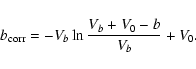
We characterize the thermistor behavior of thermometers and bolometers using
The heat equilibrium for the bolometer reads:
Table 1: Bolometer model parameters as described in Eqs. (1) and (2) for each of the Archeops bolometers.
![\begin{figure}
\par\includegraphics[angle=90, width=17cm,height=15cm]{5258f5.ps}\end{figure}](/articles/aa/full/2007/21/aa5258-06/img37.gif) |
Figure 5:
From top to bottom and from left to right: the power spectra (in
|
| Open with DEXTER | |
Table 2: For all Archeops bolometers from left to right. Photometric quantities as representative of night flight values: the current, the resistance, and the responsivity.Expected and measured absorbed power, efficiency, and photon and total noise.
Table 1 lists the parameters of all thermometers and
bolometers that were used during KS3 flight (bolometers ordered by channel,
217K05 was blind during the flight). The differential conductivity at 100 mK
is
![]() (from Eq. (2)). These
constants are consistent with those measured using cosmic ray hits. A more detailed
description of the previous issues is given in Sect. 6. The
heat capacity was simply taken as
(from Eq. (2)). These
constants are consistent with those measured using cosmic ray hits. A more detailed
description of the previous issues is given in Sect. 6. The
heat capacity was simply taken as
![]() ,
where
,
where ![]() is
the first time constant of the bolometer. Time constants are derived from a
fit on Jupiter data taken during the flight, including electronic filtering
and a Gaussian beam (see Sect. 6.1).
is
the first time constant of the bolometer. Time constants are derived from a
fit on Jupiter data taken during the flight, including electronic filtering
and a Gaussian beam (see Sect. 6.1).
The differential conductivity G is taken at
![]() .
The "Kiruna'' bolometers have typical conductivity between 60 and 80 pW/K and a heat capacity of 0.3 to 1 pJ/K, although some of them deviate significantly from this range.
.
The "Kiruna'' bolometers have typical conductivity between 60 and 80 pW/K and a heat capacity of 0.3 to 1 pJ/K, although some of them deviate significantly from this range.
We include in the detector noise model contributions from the FET electronics, the Johnson noise and the bolometer thermodynamic noise (Mather 1984). To the detector noise we quadratically add the photon noise deduced from our photometric model. The bolometer noise is not white at high frequency due to the bolometer time response. Figure 5 shows an example of power spectra of the time-ordered data of four representative Archeops bolometers during the KS3 flight. We overplot the noise model discussed above, which is in qualitative agreement without any parameter tuning at frequencies higher than a few Hz. We observe an increase in power with decreasing frequency mainly due to the low-frequency systematics. Although we have smoothed out the power spectrum we still can observe peaks that correspond to the sky signal at the spin frequency harmonics. These are mainly galactic and atmospheric emissions. Centered at 1 Hz, for the high frequency channels in particular, there is a very peculiar structure that may be of atmospheric origin. Finally, at high frequency we observe correlated structures. A more detailed description of systematics and their subtraction is given in Sect. 7.
Finally, we present a summary of the noise properties of all Archeops bolometers in Table 2. From left to right we include representative values within the night flight for the main photometric quantities of those bolometers: current, resistance, and responsivity. Next we provide the expected absorbed power from a simple photometric model made of subsystem transmission measurements presented in Sect. 3.2.1. Then we give the absorbed power as measured (with 1 pW absolute uncertainty) using the bolometer model described in Sect. 3.2.2. The efficiency is given as the ratio of the Jupiter inflight calibration to the calibration from the photometric model. Noise measurements are given at the bolometer level both for photon and total noise. The photon noise is within a factor 2 of the total noise as measured in flight conditions.
The data were acquired in total power mode via an AC square-wave
modulated bias. All the modulations are driven by the same clock at
76.3 Hz, leading to an acquisition frequency
![]() .
The AC square-wave modulated bias transformed the data into a series of
alternative positive and negative values. This induced a peak at the
Nyquist frequency,
.
The AC square-wave modulated bias transformed the data into a series of
alternative positive and negative values. This induced a peak at the
Nyquist frequency,
![]() ,
in the Fourier power spectrum of the
bolometer data. This peak dominates the signal and needs to be
removed after demodulation.
For this purpose we constructed a digital filter with the
following constraints:
,
in the Fourier power spectrum of the
bolometer data. This peak dominates the signal and needs to be
removed after demodulation.
For this purpose we constructed a digital filter with the
following constraints:
![\begin{figure}
\par\includegraphics[width=7.8cm,height=4.5cm]{5258f6.ps}\\ [1mm]
\includegraphics[width=7.8cm,height=4.5cm]{5258f7.ps}\end{figure}](/articles/aa/full/2007/21/aa5258-06/img49.gif) |
Figure 6: Top: Kernel of the digital filter used for demodulation (see text for details). Bottom: Fourier power spectrum of the digital filter compared to a square filter, to the beam pattern and to the bolometer time constant. |
| Open with DEXTER | |
![\begin{figure}
\par\includegraphics[scale=0.38,angle=90]{5258f8.ps} \end{figure}](/articles/aa/full/2007/21/aa5258-06/img50.gif) |
Figure 7: Top: Fourier power spectrum of KS3 143K01 bolometer data showing the frequency peaks produced by the readout electronic noise. Bottom: Same after preprocessing. The amplitude of the peaks is significantly reduced. |
| Open with DEXTER | |
While the on-board computer deals with in-flight commands,few data blocks are buffered
before being dumped into the flash memory.
Small offset variations in the electronics lead to
significant differences between the mean value of the last recorded
blocks and those following. As in-flight commands are sent and received
by the on-board computer periodically during the flight (every few data
blocks), the differences in the mean between blocks induce a parasitic
signal on the data. This parasitic signal shows up in the data as a
periodic pattern of frequency
![]() .
Furthermore, as series
of blocks are buffered before recording, we also observe in the data
periodic patterns at frequencies that are multiples of
.
Furthermore, as series
of blocks are buffered before recording, we also observe in the data
periodic patterns at frequencies that are multiples of
![]() .
For most of the bolometers this systematic signal
dominates the noise and is clearly visible both in the time and
frequency domain. The top panel of Fig. 7 shows a
zoom-up of the power spectrum of the data of the KS3 143K01 Archeops
bolometer. We observe a series of peaks in the spectrum that
correspond to the parasitic signal.
.
For most of the bolometers this systematic signal
dominates the noise and is clearly visible both in the time and
frequency domain. The top panel of Fig. 7 shows a
zoom-up of the power spectrum of the data of the KS3 143K01 Archeops
bolometer. We observe a series of peaks in the spectrum that
correspond to the parasitic signal.
The subtraction of the parasitic periodic signal can be easily achieved
using a time domain template for it. Indeed, we have implemented a
fast algorithm for calculating a time varying template of the parasitic
signal. First of all, for each Archeops timeline, we divide the
data into pieces of N blocks of 720 samples. The block size
corresponds to the longest period between two in-flight commands. Then
each piece of data is reordered into a
![]() matrix so
that pattern of the parasitic signal evolving in time over 720 samples
can be calculated by smoothing up over the N blocks. The exact number of
the 720-sample blocks to be summed up is a compromise between
the minimum signal to noise ratio needed for extracting the
parasitic signal from the data, the time evolution rate of the
parasitic signal, and the minimum time interval needed to
consider that the sky signal varies sufficiently for not contributing
to the template. We have found that
N=100 is a good compromise for most Archeops bolometers. The constructed template is repeated Ntimes (size in samples of the time interval processed) and then
subtracted from each piece of data.
matrix so
that pattern of the parasitic signal evolving in time over 720 samples
can be calculated by smoothing up over the N blocks. The exact number of
the 720-sample blocks to be summed up is a compromise between
the minimum signal to noise ratio needed for extracting the
parasitic signal from the data, the time evolution rate of the
parasitic signal, and the minimum time interval needed to
consider that the sky signal varies sufficiently for not contributing
to the template. We have found that
N=100 is a good compromise for most Archeops bolometers. The constructed template is repeated Ntimes (size in samples of the time interval processed) and then
subtracted from each piece of data.
The bottom panel of Fig. 7 shows the power spectrum of the KS3 143K01 bolometer after applying the above procedure, which reduces the peaks significantly. For example, the fundamental frequency peak at 2.12 Hz is reduced to much less than 10% of its original value. The peak at 12.7 Hz, although significantly reduced, is still visible in the preprocessed spectrum. It will be cut off in the Fourier domain as discussed in Sect. 7.3.
The cryostat temperature underwent a slow decrease during the flight,
leading to a slow change in calibration in
![]() .
This
change in calibration can be corrected for by modeling the responsivity of
the bolometer. Actually, for a given TOD
b in
.
This
change in calibration can be corrected for by modeling the responsivity of
the bolometer. Actually, for a given TOD
b in ![]() ,
we can write the
linearity corrected TOD as follows
,
we can write the
linearity corrected TOD as follows
 |
(3) |
In this section, we describe the identification and flagging of parasitic effects, including glitches, noise bursts, and jumps in the data. For Archeops, we call glitches those signals in the TOD related to the increase in temperature of the bolometer due to the energy deposited by cosmic-ray hits. We call jumps the step-like signals that are essentially due to changes of the equilibrium voltage of the bolometer that happen only a few times during the entire flight. We call bursts of noise signals in the TOD presenting large extra noise, which are given by microphonic noise coming mainly from the mechanical oscillations of the gondola. In the following we call spikes all those spike-like signals in the TOD well above the average noise rms. In Archeops the spikes in the data are either glitches, Galactic signal, bright point sources or point-like large noise regions.
To flag and remove the data affected by the above systematic effects,
the first step is to detect spikes in the TODs above a certain
threshold level. For this purpose the rms. noise level, ![]() 2,
is estimated locally on a 400-point running window as the standard
deviation from the median value, m, of the data after removing 5% of
the lowest and highest data values. The data deviating by more than 8
2,
is estimated locally on a 400-point running window as the standard
deviation from the median value, m, of the data after removing 5% of
the lowest and highest data values. The data deviating by more than 8![]() from the mean are considered to be glitches. To preserve the Galactic signal, which
can sometimes be spiky or/and larger than the threshold limit, a
baseline
from the mean are considered to be glitches. To preserve the Galactic signal, which
can sometimes be spiky or/and larger than the threshold limit, a
baseline
![]() is fitted as a combination of the two first Fourier
modes on the 400-point running window and is removed whenever data values
above the threshold are detected
at Galactic latitude between -10
is fitted as a combination of the two first Fourier
modes on the 400-point running window and is removed whenever data values
above the threshold are detected
at Galactic latitude between -10![]() and +10
and +10![]() .
The
value of
.
The
value of ![]() is then re-computed and the above criteria
re-applied. This technique is time-consuming but not required
outside of the Galactic plane where a flat baseline is already a very
good approximation.
is then re-computed and the above criteria
re-applied. This technique is time-consuming but not required
outside of the Galactic plane where a flat baseline is already a very
good approximation.
The second step is then to flag the data. When the parasitic
signal is due to a cosmic ray, we can model it by the convolution of a
Dirac delta function at time ti with the sampling window and a
decreasing exponential function with two time constants
![]() and
and
![]() .
The first corresponds to the
relaxation time of the bolometer itself and the second is of unknown
origin. The values of the time constants depend only on the bolometer and are assumed to
be the same for all glitches hitting this bolometer. The main objective of
this first analysis is not to reproduce the glitch shape faithfully but
to estimate which part of the data is badly affected by it and must be
flagged. Therefore, the same conservative values are adopted for all
bolometers,
.
The first corresponds to the
relaxation time of the bolometer itself and the second is of unknown
origin. The values of the time constants depend only on the bolometer and are assumed to
be the same for all glitches hitting this bolometer. The main objective of
this first analysis is not to reproduce the glitch shape faithfully but
to estimate which part of the data is badly affected by it and must be
flagged. Therefore, the same conservative values are adopted for all
bolometers,
![]() samples (13 ms) and
samples (13 ms) and
![]() samples (325 ms). We then fit the following glitch model
samples (325 ms). We then fit the following glitch model
![\begin{eqnarray*}t_{\rm min} & = & t_i - 11\\
t_{\rm max} & = & t_i
+ \tau_{\...
...{\rm long} \ln \left[\frac{A_{\rm long}}{0.1\sigma}\right]
+ 11
\end{eqnarray*}](/articles/aa/full/2007/21/aa5258-06/img68.gif)
Table 3: Statistics of glitches per minute for the KS3 flight and proportion of flagged data.
Detailed statistics of the number of cosmic rays detected in the KS3
flight are reported in Table 3. The bolometers from
the Trapani flight are quite sensitive to glitches, 15 to 20 glitches
per minute. The polarized OMT bolometers at 353 GHz shows a rate of ![]() 4 glitches per
minute, whereas we detect less than 2 glitches
per minute at 217 GHz and 545 GHz. At 143 GHz the bolometers have a glitch rate of between
1.5 and 4 per minute. The glitch rate is related to the
effective surface of the bolometer, which varies between bolometers. A
higher glitch rate can be explained by a larger effective area of the
spider-web absorber.
4 glitches per
minute, whereas we detect less than 2 glitches
per minute at 217 GHz and 545 GHz. At 143 GHz the bolometers have a glitch rate of between
1.5 and 4 per minute. The glitch rate is related to the
effective surface of the bolometer, which varies between bolometers. A
higher glitch rate can be explained by a larger effective area of the
spider-web absorber.
In the above procedure, bursts of other kinds of noises in the data are detected as glitches and the flagging obtained is poor. To ensure better flagging, we proceed to a visual inspection of the data. We check all the pieces of data found above the threshold limit and extend the flagging manually if necessary. Those data samples affected by noise bursts are flagged as such. We also observe jumps on the data that are caused by changes in the bias current of the bolometer.
The values of the bias current are stored as housekeeping data, which allows us to correct the data with jumps via a simple fitting algorithm. In addition, we determine the data samples which are affected by jumps by visual inspection and they are manually flagged. All these events occur only at the beginning and at the end of the flight.
At the end of the process, a total of 1-2.5% (resp. 2-4% and 12-18%) of the data are flagged for the KS3-like bolometers (resp. for the OMT and Trapani-like bolometers). Flagged data are then replaced by constrained realizations of noise as discussed in Sect. 8.4.
The knowledge of the pointing attitude was not needed during the flight but an accurate a posteriori reconstruction is critical for mapping the sky signal correctly. The pointing of each of the detectors in the focal plane is computed as follows. First, a pointing solution for the payload is obtained from the processing of optical data collected by the fast stellar sensor (FSS) during the flight. Finally, we estimate the pointing offset with respect to the payload axis for each bolometer using the reconstruction of the focal plane from measurements of point sources (see Sect. 6 for details).
We have developed an algorithm to extract star candidates from the FSS time-sampled photodiode signals (see Sect. 2.2). Each star candidate is kept in a table that includes its detection time, its position along the diode array and the electrical intensity observed. The position of the star candidate along the diode array is given in terms of an effective diode number. The electrical intensity measured is proportional to the logarithmic value of the flux of the star.
In the following, we use equatorial coordinates {
![]() }
to define the position of celestial objects on the sky. The FSS data
are most easily handled in local coordinates associated with the
gondola frame, for which the zenith corresponds to the gondola
spin-axis direction. The direction of a star on the celestial sphere is
then given by
}
to define the position of celestial objects on the sky. The FSS data
are most easily handled in local coordinates associated with the
gondola frame, for which the zenith corresponds to the gondola
spin-axis direction. The direction of a star on the celestial sphere is
then given by ![]() ,
the angular distance between the spin axis and
the direction of the star (hereafter the axial distance), and by
,
the angular distance between the spin axis and
the direction of the star (hereafter the axial distance), and by
![]() ,
the phase corresponding to the azimuth measured from the
North.
,
the phase corresponding to the azimuth measured from the
North.
To reconstruct the pointing direction of the gondola, we need to find
the direction of the center of the diode array. The instantaneous
pointing solution is fully described by the set {![]() ,
,
![]() ,
,
![]() }, where
}, where ![]() and
and ![]() are the
equatorial coordinates of the gondola spin axis and
are the
equatorial coordinates of the gondola spin axis and ![]() the
phase for the diode array. Note that the phase value
the
phase for the diode array. Note that the phase value ![]() is the
same for all the diodes in the array, and therefore also the same for all
detected stars, because the diode array is placed perpendicularly to
the scanning direction. In other words, the number of the diode lightened is only
given by the axial distance of the observed star.
is the
same for all the diodes in the array, and therefore also the same for all
detected stars, because the diode array is placed perpendicularly to
the scanning direction. In other words, the number of the diode lightened is only
given by the axial distance of the observed star.
The goal is to produce an optimal pointing solution as a function of time. The reconstruction is based upon the comparison between FSS data and a dedicated star catalog compiled from the Hipparcos catalog. The electrical intensity of stars in the catalog is computed by taking the FSS spectral response into account. Hereafter, we call signal a star candidate in the list produced by the FSS software and star an object taken from the star catalog. First, we find the star to be associated with each FSS signal. We then a global fit of all the associated detections to reconstruct the pointing.
To associate signals with stars, a first estimate of
the pointing solution is needed. This is obtained via the GPS data that give
the local vertical direction, corresponding to the spin-axis
direction {![]() ,
,
![]() } to an accuracy of
} to an accuracy of ![]() 1
degree, taking the gondola average pendulation of about few seconds
into account. We then
match signal and star directions and try to identify for each signal
the corresponding star. There is no direct measurement of the FSS
phase
1
degree, taking the gondola average pendulation of about few seconds
into account. We then
match signal and star directions and try to identify for each signal
the corresponding star. There is no direct measurement of the FSS
phase ![]() ,
so we need to reconstruct it from the rotation period
by integration.
,
so we need to reconstruct it from the rotation period
by integration.
We now describe the gondola motion relative to the celestial sphere.
We call a rotation period the elapsed time between two successive
detections of the same star after one revolution. Each revolution
takes about 30 s. Due to the Earth's rotation, the spin axis moves
about 5' in ![]() per revolution. Each star can thus be seen
several times by the FSS. For each signal, we look for all compatible
signals seen in the preceding revolution. A compatible signal has a
similar intensity and a nearby diode number. Time differences between
the signal and those seen in the last revolution are binned into a
histogram. The most populated bin gives us the rotation period.
Figure 8 shows the evolution of the rotation period as a
function of time for 3 hours of the KS3 flight. This evolution is
mainly due to the presence of strong stratospheric winds during the
flight.
per revolution. Each star can thus be seen
several times by the FSS. For each signal, we look for all compatible
signals seen in the preceding revolution. A compatible signal has a
similar intensity and a nearby diode number. Time differences between
the signal and those seen in the last revolution are binned into a
histogram. The most populated bin gives us the rotation period.
Figure 8 shows the evolution of the rotation period as a
function of time for 3 hours of the KS3 flight. This evolution is
mainly due to the presence of strong stratospheric winds during the
flight.
![\begin{figure}
\par\includegraphics[height=8cm,width=8.5cm,clip]{5258f9.eps} \end{figure}](/articles/aa/full/2007/21/aa5258-06/img75.gif) |
Figure 8: Rotation period evolution during the KS3 flight. |
| Open with DEXTER | |
We reconstruct the FSS phase by integrating the angular speed
![]() ,
where T is the rotation period. The resulting estimate
,
where T is the rotation period. The resulting estimate
![]() differs from the phase by a slowly varying
offset. To correct for this bias, we compare the phase of the most intense signals for each revolution with the phase of the brightest stars located in the 1.4 degree wide band scanned by the diode array during a revolution.
differs from the phase by a slowly varying
offset. To correct for this bias, we compare the phase of the most intense signals for each revolution with the phase of the brightest stars located in the 1.4 degree wide band scanned by the diode array during a revolution.
![\begin{figure}
\par\includegraphics[height=8cm,keepaspectratio=true]{5258f10.eps}\end{figure}](/articles/aa/full/2007/21/aa5258-06/img78.gif) |
Figure 9: Evolution of the distribution of phase differences between signals and bright stars for the KS3 flight. |
| Open with DEXTER | |
The analysis of phase differences
![]() -
-
![]() gives us the FSS phase offset shown in Fig. 9. The
distribution of axial distances
gives us the FSS phase offset shown in Fig. 9. The
distribution of axial distances ![]() ,
values of bright stars
associated to intense signals, allows us to adjust the geometrical
relation between the axial distance and the diode coordinates along the
array. Figure 10 shows the distribution of the axial distance
of bright stars as a function of the diode number of the corresponding
intense signal in the FSS. We see that, for each diode number, the
distribution has a well-defined peak from which we can reconstruct the
axial distance for each diode. The width of the peak is due to the
pendulation motion of the gondola.
,
values of bright stars
associated to intense signals, allows us to adjust the geometrical
relation between the axial distance and the diode coordinates along the
array. Figure 10 shows the distribution of the axial distance
of bright stars as a function of the diode number of the corresponding
intense signal in the FSS. We see that, for each diode number, the
distribution has a well-defined peak from which we can reconstruct the
axial distance for each diode. The width of the peak is due to the
pendulation motion of the gondola.
![\begin{figure}
\par\includegraphics[height=8cm,keepaspectratio=true]{5258f11.eps}\end{figure}](/articles/aa/full/2007/21/aa5258-06/img80.gif) |
Figure 10: Distribution of the axial distance of bright stars versus the diode number of the corresponding intense signals. Notice the strange behavior of the diode 26. This diode is excluded from analysis. |
| Open with DEXTER | |
The association algorithm used above is based on a comparison of the star and
signal directions. An error
![]() on the spin axis direction
(
on the spin axis direction
(
![]() ,
,
![]() )
translates into a local rotation and thus an
error on the reconstructed direction for each of the signals. The gondola
pendulation is a slowly varying function of time on scales of a few degrees.
Therefore, the error
)
translates into a local rotation and thus an
error on the reconstructed direction for each of the signals. The gondola
pendulation is a slowly varying function of time on scales of a few degrees.
Therefore, the error
![]() and the local rotation parameters are
slowly varying functions as well. In other words, signals detected within a few
degrees of each other may have a common pointing offset.
and the local rotation parameters are
slowly varying functions as well. In other words, signals detected within a few
degrees of each other may have a common pointing offset.
The matching algorithm is based on the above statement and proceeds as follows. First, for each signal, we associate stars and signals with compatible positions and intensities. Second, given a reference signal, we check whether for the N following signals there are N stars such that the corresponding shifts are close. If so, this displacement is the signature of a local rotation induced by an incorrect reconstruction of the spin axis direction or by an incorrect estimate of the FSS phase.
Free parameters like the number N of signals used or the tolerance on the angular distance between the signal and its corresponding star directions can be tuned to optimize the association efficiency. In practice, tight cuts on those parameters reduce the probability of incorrect associations, but at the same time reduce the number of correct associations available on the regions where the pointing reconstruction is bad. To improve this situation we use the fact that the FSS sees a given star during several revolutions. Once a good association is obtained we propagate this information to the whole data set using our estimate of the rotation period and thus improve the association efficiency and therefore the pointing solution.
The axial distance ![]() is the only quantity that can be measured directly.
When signals have been associated with catalog stars, it gives us
a way to reconstruct the spin axis direction. As the position of the
signal and that of its associated star must be the same, the spin axis
is therefore located on a cone centered on the star with an opening
angle
is the only quantity that can be measured directly.
When signals have been associated with catalog stars, it gives us
a way to reconstruct the spin axis direction. As the position of the
signal and that of its associated star must be the same, the spin axis
is therefore located on a cone centered on the star with an opening
angle ![]() .
Using two pairs of associations, signal-star, we can find the
direction of the spin axis. Indeed the intersection of the two cones,
one for each couple, leads to two solutions. Only one of them is
geometrically relevant. Using the whole data set, we can thus correct
the estimate of the spin axis direction during the flight. We upgrade
the FSS phase taking the new estimate of the spin axis pointing into account.
The process is used iteratively to obtain a more accurate estimate
of the pointing for the whole flight. The increase in accuracy at each
iteration allows us to use tighter cuts to get a better quality
matching between stars and signals.
.
Using two pairs of associations, signal-star, we can find the
direction of the spin axis. Indeed the intersection of the two cones,
one for each couple, leads to two solutions. Only one of them is
geometrically relevant. Using the whole data set, we can thus correct
the estimate of the spin axis direction during the flight. We upgrade
the FSS phase taking the new estimate of the spin axis pointing into account.
The process is used iteratively to obtain a more accurate estimate
of the pointing for the whole flight. The increase in accuracy at each
iteration allows us to use tighter cuts to get a better quality
matching between stars and signals.
The FSS dataset available is mainly composed of faint stars, making the above iterative solution very important. Further, calibration uncertainties on the signal get broader as the intensity decreases. The associations for the brightest stars allow us to recalibrate the FSS signals. Adding finer constraints on the intensity of the signal increases the quality of its association to a star in the catalog. This also improves the final pointing solution.
Once the signal-star associations are obtained we have a discrete
pointing solution at the times where the signal were observed.
Our purpose was to generate an optimal continuous scan path, so we have
to interpolate the pointing solution across the FSS data. This solution
should be not only interpolated, but also optimized using the data set
![]() .
To get an optimal pointing solution, we have to reconstruct
(
.
To get an optimal pointing solution, we have to reconstruct
(
![]() ,
,
![]() ,
,
![]() ),
from the
),
from the
![]() set,
where i labels a given signal-star association. This is performed by
first computing a smooth solution for the pointing and then correcting
it.
set,
where i labels a given signal-star association. This is performed by
first computing a smooth solution for the pointing and then correcting
it.
We first produce a smooth solution for the pointing (
![]() ,
,
![]() and
and
![]() )
by fitting
the set
)
by fitting
the set
![]() using a chi-square minimization.
As the set
using a chi-square minimization.
As the set
![]() is irregularly sampled in time, we obtain a generic interpolation,
is irregularly sampled in time, we obtain a generic interpolation,
![]() ,
of the pointing solution through a decomposition of the form
,
of the pointing solution through a decomposition of the form
The coefficients
![]() are obtained from the minimization of the chi-squared
are obtained from the minimization of the chi-squared
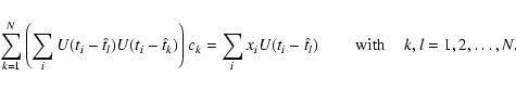
Once we have a first smooth solution for the pointing
(
![]() ,
,
![]() and
and
![]() ), we
compute corrections to it
), we
compute corrections to it
![]() ,
,
![]() ,
and
,
and
![]() .
To do this,
we decompose these 3 quantities in terms of kernel functions as in
Eq. (5). We call
.
To do this,
we decompose these 3 quantities in terms of kernel functions as in
Eq. (5). We call
![]() ,
,
![]() and
and
![]() the
decomposition coefficients for
the
decomposition coefficients for
![]() ,
,
![]() and
and
![]() ,
respectively. In
this case we consider high frequency terms to optimize the pointing solution.
,
respectively. In
this case we consider high frequency terms to optimize the pointing solution.
The FSS dataset
![]() can be
rewritten more explicitly as
can be
rewritten more explicitly as
![]() .
Here
.
Here ![]() is a
linear function of the diode number, and
is a
linear function of the diode number, and
![]() and
and
![]() are the coordinates of the star corresponding to signal
i. This set can also be expressed for the star position in gondola-frame
coordinates
are the coordinates of the star corresponding to signal
i. This set can also be expressed for the star position in gondola-frame
coordinates
![]() .
We can obtain an estimate of
the pointing corrections by comparing the reconstructed star positions with
the pointing position at the time of their observation.
.
We can obtain an estimate of
the pointing corrections by comparing the reconstructed star positions with
the pointing position at the time of their observation.
The star coordinates
![]() and
and
![]() in the
gondola frame depend on the spin axis direction. A variation
in the
gondola frame depend on the spin axis direction. A variation
![]() and
and
![]() in this
direction induces a modification of the coordinates
in this
direction induces a modification of the coordinates
![]() and
and
![]() .
To the first order, we have
.
To the first order, we have
![\begin{figure}
\par\includegraphics[height=8cm,keepaspectratio=true]{5258f12.eps}\end{figure}](/articles/aa/full/2007/21/aa5258-06/img130.gif) |
Figure 11: Scatter plot of the phase differences in degrees between signals and associated stars for each FSS diode. |
| Open with DEXTER | |
In the above we have assumed that the photodiode array was oriented
perpendicularly to the pointing direction. This hypothesis can be
verified by comparing the phase for the stars with the phase of the FSS
as a function of the diode number. This comparison is shown in
Fig. 11. We observe a phase shift that indicates that the
photodiodes array is tilted along the scan direction. Given the
1.8 m
focal length of the parabolic mirror and a 1 mm photodiode area along
the cross-can direction, we find an inclination of ![]() 3 degrees. The
phase of each signal is thus corrected to take this effect into account.
3 degrees. The
phase of each signal is thus corrected to take this effect into account.
We have two independent but complementary ways of assessing the
accuracy of the Archeops pointing reconstruction. A first estimate can
be obtained from the distribution of coordinate differences between the
signals and their associated stars. Figure 12
show the distribution of errors in the plane
axial distance-phase before and after the scan path fit. The
95% and 68% confidence level contours are displayed in white. We
observe that the axial distance coordinate has a intrinsically better
accuracy by a factor 2.5. Furthermore, we notice a significant decrease in
the errors for both the axial distance and the phase.
![\begin{figure}
\par\includegraphics[height=5cm,width=5cm]{5258f13.eps} \includegraphics[height=5cm,width=5cm]{5258f14.ps}\end{figure}](/articles/aa/full/2007/21/aa5258-06/img131.gif) |
Figure 12: From top to bottom, distribution of errors in axial distance - phase plane with 95% and 68% confidence levels (in white) before and after each scan path fit, respectively. |
| Open with DEXTER | |
We can also estimate the errors in the pointing reconstruction via the
Fisher matrix of the free parameters in the scan-path fit described by
Eqs. (8) and (9). This gives us a
continuous estimate of the pointing error that is used to flag those
regions for which the pointing is badly known. Hereafter, we call this
flag on the data the bad-pointing flag. The distribution of equatorial coordinate differences in
Fig. 13 shows that the attitude reconstruction is achieved
with an accuracy better than 1.5 and 1 arcmin in RA and Dec, respectively, at the 1-![]() level.
level.
![\begin{figure}
\par\includegraphics[height=5cm,width=5cm]{5258f15.ps} \end{figure}](/articles/aa/full/2007/21/aa5258-06/img132.gif) |
Figure 13: KS3 flight 95% end 68% confidence levels for error distribution in equatorial coordinates after the scan-path fit. |
| Open with DEXTER | |
We describe in this section the reconstruction of the Archeops focal
plane parameters for the KS3 flight. For this purpose we estimate
the time response of the bolometers, the optical response of
the photometric pixels, and
the focal plane geometry on the celestial sphere. The
focal plane is reconstructed using planet observations. The
brightest, Jupiter, was observed twice at ![]() 16.5 and
21h00 UT hours and can be considered to be a point source at the Archeops
resolution (apparent diameter of 45 by 42 arcsec). We also use Saturn
observations obtained at 15h36 and 18h427 UT hours to cross check the results.
Saturn can be also considered as a point source at the Archeops
resolution (apparent diameter of 19 by 17 arcsec).
16.5 and
21h00 UT hours and can be considered to be a point source at the Archeops
resolution (apparent diameter of 45 by 42 arcsec). We also use Saturn
observations obtained at 15h36 and 18h427 UT hours to cross check the results.
Saturn can be also considered as a point source at the Archeops
resolution (apparent diameter of 19 by 17 arcsec).
For each detector, we start by computing local maps of the planets in azimuth-elevation coordinates that correspond to the along-scan and cross-scan directions. These maps are obtained by projecting the TOD data without filtering. To remove the zero level in these maps we estimate a baseline in the TOD, which is then subtracted. The latter is estimated from a TOD where all the flagged data are interpolated using a constrained realization of noise. The TOD signal obtained for planet observations is the superposition of two main effects: first, the convolution of the source sky signal with the beam pattern of the photometric pixels, and second, the convolution of the bolometric signal with the time response of the bolometers that is characterized by a time constant. Both effects are clearly visible in the Jupiter map shown in the top panel of Fig. 14. The beam pattern convolution widens up the point-source signal both in the cross-scan and along-scan directions. The effect of the time response convolution appears as a tail in the map along the scan direction.
![\begin{figure}
\par\includegraphics[width=9cm,height=6cm]{5258f16.ps} \end{figure}](/articles/aa/full/2007/21/aa5258-06/img133.gif) |
Figure 14:
Top: map of Jupiter for the 143K03 bolometer in |
| Open with DEXTER | |
In our analysis we first estimate the bolometer time constants for each using in-scan profiles of the Jupiter or Saturn maps. We then deconvolve the TOD from these time constants and recompute local maps like the one presented in the bottom panel of Fig. 14. From these maps, we characterize the beam pattern of the photometric pixels.
The time response, TR, of the bolometers can be described by the combination of two decreasing exponentials with time constants ![]() and
and ![]()
 |
(10) |
The time constants are estimated fitting the Jupiter profiles using a
![]() minimization for a grid of 3 parameters
minimization for a grid of 3 parameters ![]() ,
,
![]() ,
and
,
and
![]() ,
which are set in the range [1, 10] ms, [10, 100] ms, and [0, 1]
respectively. The profiles used are the 4 arcmin cross-scan average of
local maps of the two Jupiter crossings. For each set of parameters,
we deconvolve the initial TOD from the
,
which are set in the range [1, 10] ms, [10, 100] ms, and [0, 1]
respectively. The profiles used are the 4 arcmin cross-scan average of
local maps of the two Jupiter crossings. For each set of parameters,
we deconvolve the initial TOD from the
![]() .
We then fit a Gaussian on the rising part of the beam profile and use a
Gaussian with the same amplitude and sigma for the decreasing part.
We fit the decay considering the lower 80% of the profile data.
.
We then fit a Gaussian on the rising part of the beam profile and use a
Gaussian with the same amplitude and sigma for the decreasing part.
We fit the decay considering the lower 80% of the profile data.
We compute the minimum of the ![]() in the (
in the (![]() ,
,
![]() ),
(
),
(![]() ,
,
![]() ), and (
), and (![]() ,
,
![]() )
planes. The best-fit
parameter values are obtained from the average of the two maxima
obtained for each parameter. We obtain
the 1
)
planes. The best-fit
parameter values are obtained from the average of the two maxima
obtained for each parameter. We obtain
the 1![]() error bars
by integrating the surface. If
error bars
by integrating the surface. If ![]() is compatible with 0 to
within 1
is compatible with 0 to
within 1![]() ,
we compute the estimation of
,
we compute the estimation of ![]() again using a
single time-constant model to reduce the error bars.
again using a
single time-constant model to reduce the error bars.
Figure 15 shows one of the Jupiter map profiles for the 217K04 bolometer before (in red) and after (in black) bolometer optical time response deconvolution. The tail in the profile due to the time response is clearly suppressed after deconvolution.
![\begin{figure}
\par\includegraphics[width=7cm,clip]{5258f17.ps} \end{figure}](/articles/aa/full/2007/21/aa5258-06/img138.gif) |
Figure 15:
217K04 Beam profile on Jupiter before (in red) and after (in black) deconvolution of the two time constants (
|
| Open with DEXTER | |
In Table 4 we present the values of
![]() ,
,
![]() ,
and
,
and
![]() for each of the Archeops bolometers obtained from analysis of the Jupiter profiles. The analysis of the Saturn profiles provides consistent results.
for each of the Archeops bolometers obtained from analysis of the Jupiter profiles. The analysis of the Saturn profiles provides consistent results.
Table 4: Bolometer time constants for the Archeops KS3 flight.
The time response of the bolometer can also be estimated using the
signal from cosmic-ray glitches with short time constant (see
Sect. 4.4) that hits the bolometer. To a very
good approximation the signal for these glitches is just the
convolution of a Dirac delta function with the bolometer time response
and the sampling kernel and so they all have the same shape. A
template of this can be obtained by piling up all short glitches in
the data after common renormalization both in position and amplitude.
We can then fit the glitch model
(Eq. (4)) to this template to estimate
![]() .
Notice that only
a few glitches have an additional, significantly long time constant
preventing us from reconstructing an accurate template.
Figure 16 shows in black the glitch template
computed for the bolometer 217K01. We trace the best glitch
model fit for it, corresponding to a time constant of
.
Notice that only
a few glitches have an additional, significantly long time constant
preventing us from reconstructing an accurate template.
Figure 16 shows in black the glitch template
computed for the bolometer 217K01. We trace the best glitch
model fit for it, corresponding to a time constant of
![]() ms.
ms.
![\begin{figure}
\par\includegraphics[width=5.5cm,clip]{5258f18.ps} \end{figure}](/articles/aa/full/2007/21/aa5258-06/img173.gif) |
Figure 16:
Glitch template for the bolometer 217K01. A single time constant
model has been fitted to the data. For the best fit, traced in red, the time
constant is
|
| Open with DEXTER | |
In Fig. 17 the values of
![]() obtained from
the fit of glitches are compared to the shorter optical time constant
obtained from
the fit of glitches are compared to the shorter optical time constant
![]() estimated using Jupiter (Table 4). These are
compatible within 1
estimated using Jupiter (Table 4). These are
compatible within 1![]() for a large number of detectors. The
observed discrepancies may be due to the intrinsic degeneracy between
time response and beam pattern and the way we break it. Equally, we
can imagine different time delays in the detector response depending on
where exactly the glitch hits.
for a large number of detectors. The
observed discrepancies may be due to the intrinsic degeneracy between
time response and beam pattern and the way we break it. Equally, we
can imagine different time delays in the detector response depending on
where exactly the glitch hits.
![\begin{figure}
\par\includegraphics[width=12cm,height=5cm]{5258f19.ps} \end{figure}](/articles/aa/full/2007/21/aa5258-06/img174.gif) |
Figure 17: Comparison between glitch and Jupiter short time constant estimates. |
| Open with DEXTER | |
The second time constants
![]() and
and ![]() differ by at least one
order of magnitude. The long time constant measured on glitches can be
interpreted as a longer thermal link for glitches that hit the immediate
surrounding of the bolometer so will not be considered in the following. In
contrast, the second optical time constant,
differ by at least one
order of magnitude. The long time constant measured on glitches can be
interpreted as a longer thermal link for glitches that hit the immediate
surrounding of the bolometer so will not be considered in the following. In
contrast, the second optical time constant, ![]() ,
must be taken into
account to accurately deconvolve from the bolometer optical time response.
,
must be taken into
account to accurately deconvolve from the bolometer optical time response.
After deconvolving the Archeops TOD from the bolometer's optical time response, we reconstruct local maps of Jupiter to estimate the beam pattern shape. The beam patterns for the Archeops photometric pixels happen to be asymmetric in particular for the multimode systems (all the 217 GHz detectors but 217K01, 217K02, and 217K05 and the two 545GHz detectors).
We model the main beam shape for each photometric pixel using the Asymfast method, described in Tristram et al. (2004). This method is based on the decomposition of the main beam shape into a linear combination of circular 2D Gaussians. This allows us to accurately and simply represent asymmetric beams and to convolve full sky maps with them in a reasonable amount of time. This is very interesting when producing simulations to estimate the beam transfer function in the spherical harmonic plane (Tristram et al. 2005b).
In the text
![\begin{figure}
\par\includegraphics[width=8.2cm,clip]{5258f20.ps} \end{figure}](/articles/aa/full/2007/21/aa5258-06/img175.gif) |
Figure 18:
From top to bottom and from left to right, for the
photometric pixel 143K03, the beam pattern map in |
| Open with DEXTER | |
The Archeops main beams have been modeled using up to 15 Gaussians. The residuals after subtraction of the model from the Jupiter local maps are less than 5%. Figure 18 shows an example of this multi-Gaussian beam modeling for the photometric pixel 143K03 using 7 circular 2D Gaussians. From top to bottom and from left to right, we show the beam pattern shape from the Jupiter local maps, its multi-Gaussian fit, the residuals, and the histogram of the residuals. The latter are shown to be compatible with Gaussian distributed noise.
Table 5: Resolution in terms of the FWHM and ellipticity of the beam pattern for the Archeops photometric pixels in the KS3 flight. See text for details.
The resolution for each of the photometric pixels has been estimated from a 2D
elliptical Gaussian fit to the local beam maps from Jupiter observations. The
FWHM values given in Table 5 are the geometric mean value in the
two directions. We also present the ellipticity as computed from the ratio
between the minor and the major axes. The optical mode of
the bolometers is indicated in the last column: S for single
mode bolometers and M for multimode bolometers.
For single-mode systems, the beamwidth is
about 11 arcmin. The multimode systems at 217 GHz and 545 GHz have larger
beams with
![]() arcmin. The 353 GHz beams are single mode but
illuminate a small part of the primary mirror to have clean
polarized beams. A degradation of the beams was noticed in the KS3
flight compared to ground-based measurements (which are close to the diffraction limit)
due to a slight change in focus as a result of the secondary mirror moving after the crash landing of the KS2 flight.
arcmin. The 353 GHz beams are single mode but
illuminate a small part of the primary mirror to have clean
polarized beams. A degradation of the beams was noticed in the KS3
flight compared to ground-based measurements (which are close to the diffraction limit)
due to a slight change in focus as a result of the secondary mirror moving after the crash landing of the KS2 flight.
No specific treatment has been applied in the data analysis to account for far side lobes, since optical modeling indicates that they are expected to be at the percent level. This level of accuracy should be sufficient as galaxy and the dipole are the only signals to couple with the CMB anisotropies on the large angular scales.
The position of each photometric pixel in the focal plane with respect
to the focal plane center (FPC) is computed using Jupiter
observations. This then allows us to build the pointing of each pixel
using the pointing reconstruction described in Sect. 5.
In practice we use the relative positions of the 2D circular Gaussians
of the Asymfast decomposition to estimate the center of the beam
in focal-plane coordinates.
Figure 19 shows the reconstruction of the Archeops focal plane in
azimuth (in-scan) and elevation (cross-scan) coordinates. The Archeops
focal plane is about 2 degrees high and 2.5 degrees wide.
![\begin{figure}
\par\includegraphics[width=6.8cm,clip]{5258f21.ps} \end{figure}](/articles/aa/full/2007/21/aa5258-06/img177.gif) |
Figure 19: Focal plane of Archeops reconstructed using Jupiter observations. |
| Open with DEXTER | |
In this section we describe in detail the main systematic effects present in the Archeops data, as well as the methods and algorithms used for their subtraction. Because of the circular scanning strategy used by Archeops, the sky signal shows up in the data at frequencies that are harmonics of the spin frequency. This naturally leads to three distinct regimes in frequency. First, the very low frequency components at frequencies well below the spin frequency (f< 0.01 Hz), which are mainly due to 1/f-like noise and systematics. Second, the spin-frequency components ( 0.03 < f < 3 Hz) at frequencies that contain most of the sky signal of interest. And finally the high-frequency components at frequencies much higher than the spin frequency (f > 10 Hz), which are dominated by detector noise.
![\begin{figure}
\par\includegraphics[height=10cm,width=17cm]{5258f22.ps} \end{figure}](/articles/aa/full/2007/21/aa5258-06/img178.gif) |
Figure 20:
Left column: from top to bottom, raw Archeops data in
|
| Open with DEXTER | |
At very low frequency the Archeops data are dominated by systematics coming mainly from temperature fluctuations of the three cryogenic stages at 100 mK, 1.6 K, and 10 K and from the variation of air mass during the flight due to changes in the balloon altitude. The left column of Fig. 20, from top to bottom, shows the raw Archeops data for the 143K03, 217K06, 353K01 and 545K01 bolometers in the period from 14h00 to 29h00 UT time. We observed a very low-frequency drift in the data which is very well correlated from bolometer to bolometer, as well as with the low-frequency components of the data from thermometers placed at each of the cryogenic stages and with measurements of the altitude of the balloon.
This drift is removed via a decorrelation analysis that uses as templates the housekeeping data described above and a fifth order polynomial defined in the time interval of interest. To compute the correlation coefficients, we first smear and undersample both the Archeops data and the templates, then perform a linear regression. A final estimate of the drift is obtained from the best-fit linear combination of the templates that are previously smoothed in order to keep only the very low frequency signal. In the left column of Fig. 20 we overplot the reconstructed very low-frequency drift for the four Archeops bolometers. In the right column of the figure we show the Archeops data after subtraction of the low-frequency drift estimate, which reduces the signal amplitude by a factor of 50. Although the decorrelation procedure is very efficient, we can still observe a correlated low-frequency parasitic signal in the bolometers. To avoid mixing of bolometer signals at this stage of the processing, this effect is considered within the map-making pipeline described in Sect. 10.
![\begin{figure}
\par\includegraphics[height=10cm,width=17cm,clip]{5258f23.ps} \end{figure}](/articles/aa/full/2007/21/aa5258-06/img179.gif) |
Figure 21:
Left column: from top to bottom, Archeops data in |
| Open with DEXTER | |
The Archeops data at the first few harmonics of the spin frequency are particularly important. They contain the large angular scale signal of the sky whose mapping is one of the main objectives of the Archeops experiment. At these frequencies, in addition to the CMB anisotropies and the Galaxy, two main components can be identified - the CMB dipole and atmospheric emission. Although the former is critical for calibrating the Archeops data at 143 and 217 GHz (see Sect. 9.1), in this analysis we remove these two contributions to obtain the galaxy and CMB anisotropy signal.
As above, we perform a decorrelation analysis to remove these parasitic
signals. A template for the dipole in mK
![]() is simulated using
the WMAP best dipole solution (Bennett et al. 2003).
The atmospheric contamination is
mainly due to the variation in the air mass induced by changes in the
altitude and the pointing elevation of the payload. As templates for
this effect, we use the housekeeping data corresponding to measurements
of the altitude of the balloon and the reconstructed elevation of the
focal plane. To compute the correlation coefficients, we smooth and
resample both the Archeops data and the templates and perform a
linear regression. The final estimate of the spin frequency
systematics are obtained from the best-fit linear combination of
templates. The left column of Fig. 21 shows from top to
bottom, the Archeops data in
is simulated using
the WMAP best dipole solution (Bennett et al. 2003).
The atmospheric contamination is
mainly due to the variation in the air mass induced by changes in the
altitude and the pointing elevation of the payload. As templates for
this effect, we use the housekeeping data corresponding to measurements
of the altitude of the balloon and the reconstructed elevation of the
focal plane. To compute the correlation coefficients, we smooth and
resample both the Archeops data and the templates and perform a
linear regression. The final estimate of the spin frequency
systematics are obtained from the best-fit linear combination of
templates. The left column of Fig. 21 shows from top to
bottom, the Archeops data in ![]() V and the reconstructed
spin frequency systematics for the 143K03, 217K06, 353K01,
and 545K05 bolometers, respectively. We see that in the low-frequency
channels the dipole contribution (exactly at the spin
frequency) dominates, while the atmospheric
emission at the high frequency is much more important and dipole becomes negligible.
V and the reconstructed
spin frequency systematics for the 143K03, 217K06, 353K01,
and 545K05 bolometers, respectively. We see that in the low-frequency
channels the dipole contribution (exactly at the spin
frequency) dominates, while the atmospheric
emission at the high frequency is much more important and dipole becomes negligible.
![\begin{figure}
\par\includegraphics[height=8cm,width=17cm,clip]{5258f24.ps} \end{figure}](/articles/aa/full/2007/21/aa5258-06/img182.gif) |
Figure 22:
From left to right and from top to bottom, the power spectrum
in |
| Open with DEXTER | |
Besides the main atmospheric signal, which is correlated with templates, there is
also a residual parasitic atmospheric signal. The latter can be
qualitatively reproduced by simulating turbulent atmospheric layers
drifting across the Archeops scanning beam. Typical gradients of half
a mK![]() over 10 degrees azimuth are observed at 545 GHz with an
evolving period of 1000 s.
over 10 degrees azimuth are observed at 545 GHz with an
evolving period of 1000 s.
![\begin{figure}
\par\includegraphics[height=8cm,width=17cm,clip]{5258f25.ps} \par\end{figure}](/articles/aa/full/2007/21/aa5258-06/img185.gif) |
Figure 23:
From left to right and from top to bottom, the power spectrum
in |
| Open with DEXTER | |
The Archeops data present, at frequencies f>5 Hz, parasitic noise that shows up on the time domain as noise bursts that are neither stationary nor Gaussian. In the Fourier plane this parasitic signal is observed in the form of well-defined, correlated structures, or peaks. This parasitic noise is very likely microphonic noise. Its contribution to the data was significantly reduced in the KS3 flight (compared to the KS1 flight) by increasing the distance between the payload and the spinning motor. The latter was placed far away in the flight chain with no rigid link between them. Figure 23 shows in black the power spectra of the Archeops low-frequency processed data for the 143K03, 217K06, 353K01, and 545K01 bolometers. Structures around 15, 22, 40 and 50 Hz are clearly visible in the power spectrum. One can also see a peak at 28.5 Hz in the power spectrum of the 353K03 bolometer data.
These structures are also observed on the power spectrum of the data from the focal plane thermometers and from the blind bolometer. Moreover, they are phase-correlated, in the temporal domain, in a number of detectors. This fact allows us to efficiently remove this parasitic noise via a decorrelation analysis in the Fourier plane, using as templates the focal-plane thermometers and the blind bolometer.
Assuming a linear model, we can write the Fourier transform of the
parasitic signal for the bolometer i as
![]() where T represent the templates described
above and
where T represent the templates described
above and
![]() is a frequency-dependent correlation
coefficient. As the parasitic signal is both localized well in time
and in frequency, we perform a regression analysis in the Fourier plane
using the windowed Fourier transform over time intervals of size L in
order to compute the correlation coefficient
is a frequency-dependent correlation
coefficient. As the parasitic signal is both localized well in time
and in frequency, we perform a regression analysis in the Fourier plane
using the windowed Fourier transform over time intervals of size L in
order to compute the correlation coefficient
![]() .
To maximize
the efficiency of the algorithm and to limit the subtraction of sky
signal, which may be accidentally correlated with the templates, we apply
the decorrelation analysis only in a few predefined frequency intervals
where the parasitic signal dominates. Further, to obtain a robust
estimate of the correlation coefficient, we average it over N time
intervals so that, for each of the frequency intervals, it reads
.
To maximize
the efficiency of the algorithm and to limit the subtraction of sky
signal, which may be accidentally correlated with the templates, we apply
the decorrelation analysis only in a few predefined frequency intervals
where the parasitic signal dominates. Further, to obtain a robust
estimate of the correlation coefficient, we average it over N time
intervals so that, for each of the frequency intervals, it reads
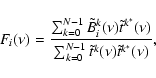 |
(11) |
The estimate of the high frequency parasitic noise is then subtracted from the data in the Fourier plane. We repeat this analysis for each of the available templates. The choice of the parameters of the method, i.e. L, N, result in a trade-off: we want to minimize the parasitic power in the TOD spectrum, but we also want that the CMB signal to remain unaffected by the process. Simulations lead to a best choice of parameters L=32 768 samples and N=32 to get a CMB power suppressed by less than 1%.
In Fig. 23 we plot the power spectra for the bolometers 143K03, 217K06, 353K01, and 545K01 before and after subtraction of the high-frequency parasitic signals. We observe that the parasitic signal is significantly reduced, in particular at the lowest frequencies. However, for most of the bolometers around 40 Hz, the processing, although efficient in removing the systematic effect, is not satisfactory (residuals are much larger than for lower frequencies). Therefore, in the following, the Archeops TODs are low-pass filtered at 38 Hz before any scientific analysis. We also observe that, in some of the bolometers, localized peaks in the spectrum are not removed in our process. These peaks are manually characterized and the signal at their frequencies is removed in the Fourier domain for all Archeops bolometers.
![\begin{figure}
\par\includegraphics[height=8.5cm,width=10cm,angle=90,clip]{5258f...
...\includegraphics[height=8.5cm,width=10cm,angle=90,clip]{5258f27.eps}\end{figure}](/articles/aa/full/2007/21/aa5258-06/img190.gif) |
Figure 24: Left column: from top to bottom, time-frequency representation in linear color scale of the 217T04 bolometer data and of the expected Galactic signal for it. Right column: same for the 217K04 bolometer. |
| Open with DEXTER | |
We have performed a time-frequency analysis of the Archeops data using the Discrete Wavelet Packet Transform (DWPT) as described in Macías-Pérez & Bourrachot (2006). The top left panel of Fig. 24 shows the power distribution in the time-frequency plane for the data of the 217T04 bolometer. At low frequency and because of the particular scanning strategy of Archeops, we can see spikes and some broader structures, which mainly correspond to the Galactic signal. This is clearly shown by the bottom plot where we trace the expected Galactic signal for this bolometer. Also at low frequency we distinguish the atmospheric residuals and the 1/f-like noise on the bolometer. We can further see, from 20 to 40 Hz, structures that vary with time and that are particularly strong around 21h00 UT. These structures are residuals, after subtraction, of the high-frequency systematics described above. Notice that the level of the systematics is significantly greater than the high-frequency noise, making this bolometer useless for scientific purposes.
On the top right panel of Fig. 24 we present the time-frequency analysis of the 217K04 bolometer. As above, we can clearly distinguish the Galaxy contribution at low frequencies, whose template is represented in the bottom right panel. We see that for this bolometer no intermediate frequency structures like that present in the previous bolometer. The systematic contribution has been significantly reduced by the high-frequency subtraction, and the residuals are well below the high frequency noise. This simple but efficient analysis allows us to exclude those bolometers that present either strong or highly time-variable systematic residuals from the further processing. Typically, all Trapani bolometers show a large amount of contamination and were excluded.
On the top panel of Fig. 24, at very high frequency we can
distinguish a slow decrease in the noise power with time, which is the main
cause of non stationarity in the Archeops data. This is due, as discussed in
Sect. 7.1, to the sudden increase in temperature of the
Archeops cryostat when taking off and to its slow cooling down to the nominal
value of about 95 mK during the f58light. To account for this non stationarity
we modeled the Archeops data as a time modulated-stationary wavelet
process (Macías-Pérez & Bourrachot 2006). These processes correspond to a continuous
generalization of piece-wise stationary processes. They are described by two
main variables: the mean power spectrum of the data and a time varying
function, ![]() (t), which account for the time variations in the power
spectrum.
(t), which account for the time variations in the power
spectrum.
![\begin{figure}
\par\includegraphics[angle=90,height=9cm,width=9cm,clip]{5258f28.ps}\end{figure}](/articles/aa/full/2007/21/aa5258-06/img191.gif) |
Figure 25:
Top: Average wavelet power spectrum in |
| Open with DEXTER | |
Figure 25 shows, in the top and bottom panels, the
time-averaged wavelet spectrum and the
![]() function,
respectively, for the noise of bolometer 217K04. In the top plot we can
clearly distinguish the increase in noise power with frequency that is
due to the deconvolution from bolometer time response. In the
function,
respectively, for the noise of bolometer 217K04. In the top plot we can
clearly distinguish the increase in noise power with frequency that is
due to the deconvolution from bolometer time response. In the
![]() function, there are two distinct regimes corresponding first to a
fast cooling of the cryostat in the first two hours and then to a
roughly constant temperature of the focal plane during the last 10
hours of flight. Notice that our estimate of
function, there are two distinct regimes corresponding first to a
fast cooling of the cryostat in the first two hours and then to a
roughly constant temperature of the focal plane during the last 10
hours of flight. Notice that our estimate of
![]() is noisy and
therefore we generally smooth it for further processing. We can also
see variations in
is noisy and
therefore we generally smooth it for further processing. We can also
see variations in
![]() above the noise limit for the second
regime, which, although small with respect to those in the first two
hours of flight, need to be taken into account in any further
processing.
above the noise limit for the second
regime, which, although small with respect to those in the first two
hours of flight, need to be taken into account in any further
processing.
Up to now, we have only considered the power spectrum evolution to define the level of the stationarity of the data. To be complete in our analysis we first have to characterize the Gaussianity of the noise distribution function and second to check its evolution in time. In practice and to reduce the uncertainties in the analysis, it is more convenient to proceed with the latter first.
We implemented a Kolmogorov-Smirnov test in the Fourier domain to check the evolution in time of the noise distribution function of each of the bolometers. Notice that the intrinsic bolometer noise can be considered Gaussian to a very good approximation, and therefore any changes on the distribution function of the noise will indicate the presence of significant residuals from systematics. We work in the Fourier domain both to speed up the calculations and to isolate the noise, which dominates at intermediate and high frequencies. We performed the test in consecutive time intervals of about 7 min that we compare two by two. We divided the frequency space in bins of 1 Hz. The test is considered to fail when the probability of having a greater Kolmogorov-Smirnov statistic under the equal distribution hypothesis is less than 1%.
![\begin{figure}
\par\includegraphics[scale=0.25,angle=90]{5258f29.ps}\\ [1.5mm]
...
...31.ps}\\ [1.5mm]
\includegraphics[scale=0.25,angle=90]{5258f32.ps} \end{figure}](/articles/aa/full/2007/21/aa5258-06/img193.gif) |
Figure 26: From top to bottom, results of the Kolmogorov-Smirnov test on the bolometers 143K03, 217K06, 353K06, and 545K01, respectively. The white polygons correspond to intervals in the time frequency plane where the test is considered to fail (see text for details). |
| Open with DEXTER | |
The results of the test for the KS3 bolometers 143K03, 217K06, 353K06, and
545K01 are shown in Fig. 26, being the white points the failing
intervals in the time-frequency domain. Between 16h00 and 27h00 UT, the test
is successful except for the lowest frequency bins (![]() Hz), in which
the Galactic and atmospheric signals, which are neither Gaussian nor
stationary, dominate. We notice that elsewhere the number of points where the
test fails is no more than 1% of the total. That is exactly what is expected
under the hypothesis of no time evolution of the distribution function.
Moreover, they do not exhibit any clustering. Around 28h00 UT, the sunrise on
the gondola induces strong time evolution due to the heating of the 10 K stage.
Hz), in which
the Galactic and atmospheric signals, which are neither Gaussian nor
stationary, dominate. We notice that elsewhere the number of points where the
test fails is no more than 1% of the total. That is exactly what is expected
under the hypothesis of no time evolution of the distribution function.
Moreover, they do not exhibit any clustering. Around 28h00 UT, the sunrise on
the gondola induces strong time evolution due to the heating of the 10 K stage.
In the range from 16h00 to 27h00 UT, as the properties of the distribution
function do not vary, we can globally study the Gaussianity of the noise.
For this purpose we have implemented a simple test in the
Fourier domain by fitting a Gaussian to the histogram of the coefficients of the Fourier
decomposition of the time ordered data that were binned in 1 Hz intervals as above
and by computing the ![]() value for the fit.
We consider the test to fail if for Gaussian distributed data the probability of having a greater
reduced
value for the fit.
We consider the test to fail if for Gaussian distributed data the probability of having a greater
reduced ![]() than the one measured is significantly below 5%.
Figure 27 shows the results of the test for the KS3
bolometers, 143K03, 217K06, 353K06, and 545K01. We trace the reduced
than the one measured is significantly below 5%.
Figure 27 shows the results of the test for the KS3
bolometers, 143K03, 217K06, 353K06, and 545K01. We trace the reduced
![]() as a function of the frequency bin. We
overplot the
as a function of the frequency bin. We
overplot the ![]() values for which the probability of having a higher
value considering a Gaussian distribution is 95% and 5%, respectively. The
reduced
values for which the probability of having a higher
value considering a Gaussian distribution is 95% and 5%, respectively. The
reduced ![]() measured are almost everywhere below or around the 5% limit,
except in the first frequency bin where the Galactic signal, highly non
Gaussian, dominates. We can therefore consider that the data are compatible with Gaussianity in a first approximation.
measured are almost everywhere below or around the 5% limit,
except in the first frequency bin where the Galactic signal, highly non
Gaussian, dominates. We can therefore consider that the data are compatible with Gaussianity in a first approximation.
We performed noise simulations, which we call constrained realizations of noise, to fill the gaps in the data. In this case we used a simple algorithm. First, we reconstructed the low-frequency noise contribution via interpolation within the gap using an irregularly sampled Fourier series. Finally, we computed the noise power spectrum locally (in time intervals of about 1 h around the gap) at high frequency and then produce a random realization of this spectrum. Note that we are only interested in keeping the global spectral properties of the data. Moreover, the gaps are in general very small in time compared to the piece of the data used for estimating the power spectrum, so this simple approach is accurate enough.
For the first estimate of the CMB angular power spectrum with the Archeops
data (Benoît et al. 2003a), we needed an accurate estimate of the noise angular
power spectrum. For this purpose, we have estimated the time power spectrum
of the noise for each of the Archeops bolometers using the algorithm described
in Amblard & Hamilton (2004). This algorithm relies on the iterative
reconstruction of the noise by subtracting in the TOD an estimate of the sky
signal. The latter is obtained from a coadded map, which at each iteration is
improved by taking the noise contribution into account. From the
reconstructed noise timeline, we can then obtain for each bolometer both the
average noise power spectrum and the ![]() function described in
Sect. 8.2. Since the noise in the Archeops data can be
considered as Gaussian-distributed (Sect. 8.3),
these two quantities are enough to simulate noise timelines using the
algorithm presented in Macías-Pérez & Bourrachot (2006). The fake timelines can then be
projected onto maps for the estimate of the noise angular power spectrum. In
general a few hundred simulations are needed to obtain a reasonable estimate.
function described in
Sect. 8.2. Since the noise in the Archeops data can be
considered as Gaussian-distributed (Sect. 8.3),
these two quantities are enough to simulate noise timelines using the
algorithm presented in Macías-Pérez & Bourrachot (2006). The fake timelines can then be
projected onto maps for the estimate of the noise angular power spectrum. In
general a few hundred simulations are needed to obtain a reasonable estimate.
![\begin{figure}
\par\includegraphics[scale=0.5,angle=90]{5258f33.ps} \end{figure}](/articles/aa/full/2007/21/aa5258-06/img195.gif) |
Figure 27:
From left to right and up to bottom, maximum reduced |
| Open with DEXTER | |
At low frequencies, the CMB dipole is a very good absolute calibrator
(Piat et al. 2003; Cappellini et al. 2003) that therefore
constitutes the primary absolute calibration of the Archeops data.
Here we used the total dipole which is the sum of the solar dipole
(constant in time) and the Earth induced dipole (with annual variations
due to the Earth's change in velocity) computed at the time of flight.
Indeed, the dipole calibration has the following advantages: 1) the dipole is spread over the whole sky, so it is always present
whatever the pointing, 2) it is much brighter (typically a factor of
100) than the CMB anisotropies, but still faint enough so that non
linearity corrections are usually not needed; and finally 3) it has the
same electromagnetic spectrum as the CMB anisotropies so that no color
corrections need be applied. The only drawback is that we must
assume a constant response for the instrument throughout a wide range
of angular scales, i.e. an extrapolation from ![]() to 1000.
The dipole being an extended source, we need to account for the beam and
the spectral transmission of each of the detectors to generate the
point-source calibration.
to 1000.
The dipole being an extended source, we need to account for the beam and
the spectral transmission of each of the detectors to generate the
point-source calibration.
In the Archeops case, the dipole signal is expected to contribute only to the
fundamental rotation frequency
![]() .
However, the drift of the rotation axis during the flight leads to a
broadening of the
.
However, the drift of the rotation axis during the flight leads to a
broadening of the
![]() dipole contribution, which needs to
be taken into account. Furthermore, as discussed in Sect. 7.2, other signals show up at the spin frequency, including both
Galactic and atmospheric signals. To account for these, we
computed the total dipole calibration coefficients from the correlation
analysis described in Sect. 7.2. We actually
produced templates of the Galactic emission using
extrapolation of the dust emission to the Archeops frequency
(Finkbeiner et al. 1999) and templates for the atmospheric emission
using the housekeeping data from
the altitude and elevation of the balloon. The template for the total
dipole in the time domain was obtained by using the Archeops
pointing to deproject a simulated CMB dipole map for which the dipole
amplitude and direction were taken from the WMAP results (Bennett et al. 2003)
dipole contribution, which needs to
be taken into account. Furthermore, as discussed in Sect. 7.2, other signals show up at the spin frequency, including both
Galactic and atmospheric signals. To account for these, we
computed the total dipole calibration coefficients from the correlation
analysis described in Sect. 7.2. We actually
produced templates of the Galactic emission using
extrapolation of the dust emission to the Archeops frequency
(Finkbeiner et al. 1999) and templates for the atmospheric emission
using the housekeeping data from
the altitude and elevation of the balloon. The template for the total
dipole in the time domain was obtained by using the Archeops
pointing to deproject a simulated CMB dipole map for which the dipole
amplitude and direction were taken from the WMAP results (Bennett et al. 2003)
The left panel of Fig. 28 shows the simulated total dipole map in Galactic coordinates for the Archeops coverage and centered in the Galactic anticenter. In the right panel we plot the Archeops reconstructed CMB dipole for the 143K03 bolometer. We see good agreement between the two maps except for some stripes when crossing the Galactic plane and on the North at high Galactic latitude.
| |
Figure 28: From left to right, simulated and reconstructed CMB dipole maps in linear scale for the Archeops 143K03 bolometer centered on the Galactic anticenter. To reconstruct both dipole maps, the timelines have been band-pass filtered. This introduces discontinuities on the maps due to the scanning strategy. |
| Open with DEXTER | |
The CMB dipole is detected with a signal-to-noise better than 500 for
12 hours of data on the 143 and 217 GHz channels. The errors on the dipole
calibration coefficients come mostly from systematic effects. We produced
several versions of the calibration coefficients by changing the templates
used in the fit. We noticed that the result is very stable compared to
even the most extreme cases. From those tests, we can deduce that the overall
(![]() )
uncertainties are 4% and 8% for the 143 and 217 GHz, respectively.
The greater uncertainty for the 217 GHz channel reflects
the spectrum of the atmospheric contamination. Notice that the dipole
calibration is performed in the early stages of the analysis before removing
the spin frequency systematics (see Sect. 7). When applied
to the 353 GHz channel, there is a residual contaminant at the same level as
the dipole. Considering the 545 GHz channel in the analysis can help in this
case and allows us to find the dipole calibration coefficient at 353 GHz, in
agreement with the Galactic calibration coefficients to within 20%, as described
below.
)
uncertainties are 4% and 8% for the 143 and 217 GHz, respectively.
The greater uncertainty for the 217 GHz channel reflects
the spectrum of the atmospheric contamination. Notice that the dipole
calibration is performed in the early stages of the analysis before removing
the spin frequency systematics (see Sect. 7). When applied
to the 353 GHz channel, there is a residual contaminant at the same level as
the dipole. Considering the 545 GHz channel in the analysis can help in this
case and allows us to find the dipole calibration coefficient at 353 GHz, in
agreement with the Galactic calibration coefficients to within 20%, as described
below.
At 353 and 545 GHz, Galactic emission is used to
calibrate the Archeops data. The best data, in term of spectral coverage and
absolute calibration accuracy, are the FIRAS spectra (Mather et al. (1990)).
FIRAS, on board the COBE satellite, was a scanning Michelson interferometer
that provided low-resolution spectra in a low (2-20 cm-1) and high
(20-100 cm-1) frequency band, for 98.7% of the sky. For individual
pixels, the signal-to-noise ratio of the FIRAS spectra was about 1 at high
Galactic latitude and ![]() 50 in the Galactic plane. The FIRAS maps used here
were obtained by fitting each FIRAS spectrum using a modified Black Body with
a
50 in the Galactic plane. The FIRAS maps used here
were obtained by fitting each FIRAS spectrum using a modified Black Body with
a
![]() emissivity law and extrapolating the fit to Archeops
frequencies. Since we were searching for the best representation of the data
and not for physical dust parameters, we restricted the fit to the frequency
range of interest, (which avoids the need for a second dust component, of the
type proposed by Finkbeiner et al. 1999). The FIRAS brightness maps are then
converted to photometric maps with the flux convention of constant
emissivity law and extrapolating the fit to Archeops
frequencies. Since we were searching for the best representation of the data
and not for physical dust parameters, we restricted the fit to the frequency
range of interest, (which avoids the need for a second dust component, of the
type proposed by Finkbeiner et al. 1999). The FIRAS brightness maps are then
converted to photometric maps with the flux convention of constant
![]() .
To
compare to the FIRAS maps and to maintain the best possible photometric
integrity, the Archeops data are convolved by the FIRAS beam and put into the
FIRAS Quadrilateralized Spherical Cube (QSC). At this stage, we have Archeops
maps at the FIRAS resolution that can be directly compared to the FIRAS
maps at the Archeops frequencies in order to derive the Galactic calibration factors.
.
To
compare to the FIRAS maps and to maintain the best possible photometric
integrity, the Archeops data are convolved by the FIRAS beam and put into the
FIRAS Quadrilateralized Spherical Cube (QSC). At this stage, we have Archeops
maps at the FIRAS resolution that can be directly compared to the FIRAS
maps at the Archeops frequencies in order to derive the Galactic calibration factors.
Due to its high signal-to-noise ratio and size, the Galactic plane is
the best place to derive the calibration factors. We computed Galactic
latitude profiles of both maps (
![]() )
at selected longitudes and performed
a best straight-line fit to the Archeops-FIRAS profile correlation from which
we derived the calibration factor and its error bar. An example of this fit is
shown in Fig. 29, where we observe a linear correlation
between the Archeops and FIRAS profile intensities. The whole calibration
process gives calibration factors with statistical errors of about 6%.
Details on the whole calibration process are given can be found in Lagache & Douspis (2006).
)
at selected longitudes and performed
a best straight-line fit to the Archeops-FIRAS profile correlation from which
we derived the calibration factor and its error bar. An example of this fit is
shown in Fig. 29, where we observe a linear correlation
between the Archeops and FIRAS profile intensities. The whole calibration
process gives calibration factors with statistical errors of about 6%.
Details on the whole calibration process are given can be found in Lagache & Douspis (2006).
![\begin{figure}
\par\includegraphics[scale=0.5]{5258f36.ps}\end{figure}](/articles/aa/full/2007/21/aa5258-06/img204.gif) |
Figure 29: FIRAS/Archeops Galactic profiles correlation on the Galactic plane (bolometer 353K01 at 353 GHz). Fitting a straight line gives the calibration factor. |
| Open with DEXTER | |
Our procedure has been extensively tested. We applied the calibration
scheme to the comparison between the FIRAS and DIRBE data at 140 and 240 ![]() m and found results in very good agreement with those of Fixsen et al. (1997).
We also tested our procedure on the Finkbeiner et al. (1999) maps, although these
maps exclude the Galactic plane below
m and found results in very good agreement with those of Fixsen et al. (1997).
We also tested our procedure on the Finkbeiner et al. (1999) maps, although these
maps exclude the Galactic plane below
![]() .
We obtained gain
differences that are less than 6% across the Archeops frequencies. We also
used Archeops maps obtained using different low-frequency filters to test the
effect of the filtering on the calibration. We found that
it modifies the calibration factors by only
.
We obtained gain
differences that are less than 6% across the Archeops frequencies. We also
used Archeops maps obtained using different low-frequency filters to test the
effect of the filtering on the calibration. We found that
it modifies the calibration factors by only ![]() 3%.
3%.
Although the calibration on the Galaxy is less accurate for the low-frequency
than for the high-frequency channels of Archeops, we can compare the CMB dipole
and Galaxy calibration factors in Fig. 30. We see
good agreement between both calibrations, with a mean ratio of the
calibration factors lower than 1.05 and all of them compatible with 1 within
the 1![]() error bars. This clearly demonstrates the robustness of the
methods used for the extended emission calibration and the consistency of the
data reduction from TODs (dipole calibration) to maps (Galactic calibration).
error bars. This clearly demonstrates the robustness of the
methods used for the extended emission calibration and the consistency of the
data reduction from TODs (dipole calibration) to maps (Galactic calibration).
![\begin{figure}
\par\includegraphics[scale=0.5]{5258f37.ps} \end{figure}](/articles/aa/full/2007/21/aa5258-06/img207.gif) |
Figure 30:
Comparison of the Galactic and Dipole calibration factors
(in
|
| Open with DEXTER | |
We also performed a point-source calibration using the measurements at the two independent crossings of the planets Jupiter and Saturn (5 times fainter than Jupiter).
For this purpose we proceed as follows: 1) We obtain the beam pattern
shape from the Jupiter measurements after deconvolution from the bolometer time response 2) We compute the flux of the sources (in ![]() V) using pixel photometry up to a radius of 40 arcmin starting from the center of the beam pattern. 3) Finally, we compare the fluxes
to a model of the temperature emission of the sources (Moreno 1998) that reproduces radio observations of Jupiter and Saturn from 20 to 900 GHz. Taking uncertainties on the
model into account, absolute errors on point-source calibration with Jupiter are estimated to be
V) using pixel photometry up to a radius of 40 arcmin starting from the center of the beam pattern. 3) Finally, we compare the fluxes
to a model of the temperature emission of the sources (Moreno 1998) that reproduces radio observations of Jupiter and Saturn from 20 to 900 GHz. Taking uncertainties on the
model into account, absolute errors on point-source calibration with Jupiter are estimated to be ![]() 12%.
12%.
The ratio between brightness temperatures at a given frequency when measured for Jupiter and Saturn
does not depend on the absolute instrument calibration. We find ratios of
![]() and
and
![]() at 143 and 217 GHz, respectively, which are not compatible with the one measured by Goldin et al. (1997) (
at 143 and 217 GHz, respectively, which are not compatible with the one measured by Goldin et al. (1997) (
![]() )
at a similar frequency (171 GHz). Due to the strong brightness
of Jupiter (about 1 K
)
at a similar frequency (171 GHz). Due to the strong brightness
of Jupiter (about 1 K![]() equivalent brightness), we expect some non-linearity in the
detection chain that could be the cause of this difference. This problem in addition to the uncertainties on the knowledge of the beam pattern and in particular of the far side lobes could also explain the small discrepancies between the Jupiter calibration and the dipole calibration as shown in Fig. 31.
equivalent brightness), we expect some non-linearity in the
detection chain that could be the cause of this difference. This problem in addition to the uncertainties on the knowledge of the beam pattern and in particular of the far side lobes could also explain the small discrepancies between the Jupiter calibration and the dipole calibration as shown in Fig. 31.
![\begin{figure}
\par\includegraphics[height=5cm,width=8cm]{5258f38.ps} \end{figure}](/articles/aa/full/2007/21/aa5258-06/img211.gif) |
Figure 31: Comparison of the point-source (Jupiter and Saturn) and dipole calibration factors. The error bars are about 4% and 8% for calibration on the dipole at 143 and 217 GHz respectively and about 12% for the calibration on the sources (essentially due to the uncertainty of the thermal emission model). |
| Open with DEXTER | |
The qualitative agreement between Jupiter calibration and the dipole primer calibration indicates that the instrumental main beam pattern is well understood.
The polarization signal for experiments like Archeops was reconstructed, as a first approximation, from the differences between pairs of bolometers (see Sect. 10.3); therefore, the accuracy of this reconstruction is very sensitive to the relative calibration between bolometers. In the case of the Archeops 353 GHz polarized channels, the absolute calibration on the Galaxy presented above is not accurate enough for the direct reconstruction of the polarized maps. Thus, we implemented a relative calibration algorithm based on the inter-comparison of Galactic profiles at constant Galactic longitude for all bolometers in the same channel. This algorithm was also applied to the unpolarized channels at 143 and 217 GHz as a cross check of the absolute calibration analysis.
Assuming N bolometers per channel, we can measure N Galactic profiles as a
function of the Galactic latitude, b,
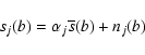
![\begin{figure}
\par\mbox{\includegraphics[width=4.3cm, height=5cm]{5258f39.ps} \includegraphics[width=4.3cm, height=5cm]{5258f40.ps} }
\end{figure}](/articles/aa/full/2007/21/aa5258-06/img215.gif) |
Figure 32:
From left to right, Archeops Galactic profiles in |
| Open with DEXTER | |
The profiles were
obtained by averaging the signal samples within latitude bins. The
errors are computed assuming that the noise is white, uncorrelated
between bolometers, and stationary. The noise in each sample is either
estimated from data outside the Galactic plane (
![]() )
or high-pass filtered data above 10 Hz (where the Galactic
signal is negligible). Results are very similar in the two methods
whose differences are less than 3% and induces negligible difference in
intercalibration coefficients. Finally, care was
taken to use the same sky coverage for all bolometers when
computing the Galactic profiles.
)
or high-pass filtered data above 10 Hz (where the Galactic
signal is negligible). Results are very similar in the two methods
whose differences are less than 3% and induces negligible difference in
intercalibration coefficients. Finally, care was
taken to use the same sky coverage for all bolometers when
computing the Galactic profiles.
For the polarized channels, the presence of strongly polarized regions on the sky may affect the computation of the intercalibration coefficients. To avoid this, we proceeded in two steps. First, we computed the relative calibration coefficients and mean Galactic profile on the full common sky area for the six polarized bolometers. Using these coefficients we built polarization maps and labeled strong polarized areas, which are then excluded from the analysis. We then rebuilt the Galactic profiles and recomputed the relative calibration coefficients. After two iterations, we observed that the estimates of the intercalibration coefficients were stable. We show the results of this analysis in Fig. 32 for the 353 GHz channel. From left to right we plot the Galactic profiles before and after intercalibration, respectively. We see that the intercalibration is achieved with a high degree of precision.
Final results on the intercalibration coefficients for the Archeops
data are given in Table 6 for all the bolometers at
143 GHz, 217 GHz (unpolarized), and 353 GHz (polarized). The
![]() statistical errors on the relative calibration coefficients
are at most 2.5% and always below 1% for the polarized channel.
Error bars are smaller at high frequency because the Galaxy signal is
stronger.
statistical errors on the relative calibration coefficients
are at most 2.5% and always below 1% for the polarized channel.
Error bars are smaller at high frequency because the Galaxy signal is
stronger.
Table 6: Relative calibration coefficients and their relative statistical errors from Galactic profiles at constant Galactic longitude.
Table 7: The Archeops KS3 in-flight timeline sensitivities per channel.
Using the observed response and white-noise level of the bolometers, we
can now estimate the global efficiency of the instrument during the KS3
flight. Table 7 gives the instrument
sensitivities in various units at the timeline level.
The best bolometers on each frequency channel are optimally
combined (
![]() )
to obtain a sensitivity at the instrument
level. From left to right the units correspond to a Rayleigh-Jeans spectrum, then a
constant
)
to obtain a sensitivity at the instrument
level. From left to right the units correspond to a Rayleigh-Jeans spectrum, then a
constant ![]() spectrum, and a CMB spectrum. Sensitivity
to the SZ effect is measured with the dimensionless y Compton
parameter. To convert to 1
spectrum, and a CMB spectrum. Sensitivity
to the SZ effect is measured with the dimensionless y Compton
parameter. To convert to 1![]() and to one-second integration,
we can simply divide by
and to one-second integration,
we can simply divide by ![]() :
see an example in the last
column.
We note that the instanteneous, single-bolometer sensitivities are among
the best ever obtained. This can be easily understood, as Archeops is above
of the atmosphere and is one of the few bolometric experiments that it is cold to
100 mK.
This places
Archeops within the best range of instrumental instantaneous
sensitivities for millimetre continuum measurements.
We also compute the averaged sensitivity, quoted in Table 8, by
using a total integration time of 12 h and a total sky coverage of
30%. The best bolometers on each frequency channel are
optimally combined (
:
see an example in the last
column.
We note that the instanteneous, single-bolometer sensitivities are among
the best ever obtained. This can be easily understood, as Archeops is above
of the atmosphere and is one of the few bolometric experiments that it is cold to
100 mK.
This places
Archeops within the best range of instrumental instantaneous
sensitivities for millimetre continuum measurements.
We also compute the averaged sensitivity, quoted in Table 8, by
using a total integration time of 12 h and a total sky coverage of
30%. The best bolometers on each frequency channel are
optimally combined (
![]() )
to obtain a sensitivity at the map
level. A square pixel of 20 arcmin is taken to compute the
average 1
)
to obtain a sensitivity at the map
level. A square pixel of 20 arcmin is taken to compute the
average 1![]() noise. The KS3 flight roughly covered 30% of the
total sky, which represent 110 000 pixels. One bolometer observed a
pixel on the map during an average time of 0.4 s.
In this case Archeops is not among the best experiments,
because the sensitivity per pixel is diluted by the large covering area
needed for reconstructing the large angular scales on the sky.
noise. The KS3 flight roughly covered 30% of the
total sky, which represent 110 000 pixels. One bolometer observed a
pixel on the map during an average time of 0.4 s.
In this case Archeops is not among the best experiments,
because the sensitivity per pixel is diluted by the large covering area
needed for reconstructing the large angular scales on the sky.
Table 8: The Archeops KS3 in-flight map sensitivities per channel.
In this section we describe how we obtained submillimetre sky maps from the Archeops timelines and pointing information. Prior to projection we remove low-frequency drifts on the Archeops timelines via a destriping algorithm. Then, these timelines are processed in three different ways to produce after projection: CMB, Galactic intensity, and polarization maps.
![\begin{figure}
\par\includegraphics*[height=8.cm,keepaspectratio=true,angle=90]{...
...ludegraphics*[height=8.cm,keepaspectratio=true,angle=90]{5258f42.ps}\end{figure}](/articles/aa/full/2007/21/aa5258-06/img226.gif) |
Figure 33: Left: power spectrum of the time-ordered data of the bolometer 545K01 before (black) and after (red) destriping. Right: zoom-in of the left plot at first multiples of the spinning frequency. |
| Open with DEXTER | |
Even after the subtraction of the very high and low-frequency,
identified systematic effects from the data, we can observe residual
stripes on the Archeops simple coadded maps. These are mainly due to
low-frequency drifts in the data coming from atmospheric residuals and
other thermal backgrounds. Notice that there is no electronic 1/fcomponent because of the AC bolometer modulation scheme (see
Sect. 4.2). To remove those drifts we
implemented a destriping algorithm (Bourrachot 2004) making the
assumption that the scanning direction is generally not related to the
orientation of the structures on the sky.
To destripe we computed a low-frequency baseline in the timelines by
minimizing the ratio
between the rms in the cross-scan and in the in-scan directions
directly from the time-ordered data (no reconstruction of maps is
needed). To represent the baseline, we used a basis of localized
functions Uk(t) where
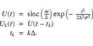 |
(12) |
The minimization was performed outside the Galactic plane over boxes
with sizes related to ![]() (typically a few tens of square degrees).
The cut on the Galactic plane is obtained from a Galactic mask derived
from Galactic template maps computed at the Archeops frequencies
(using Finkbeiner et al. 1999). The
algorithm is applied in steps of decreasing
(typically a few tens of square degrees).
The cut on the Galactic plane is obtained from a Galactic mask derived
from Galactic template maps computed at the Archeops frequencies
(using Finkbeiner et al. 1999). The
algorithm is applied in steps of decreasing ![]() (4000, 1000, 500,
and 300) to focus on different frequency ranges. In any case, data
at frequencies above 1 Hz are not affected by this method. Prior to
this process, we generally applied a classical destriping algorithm based on the
minimization of the variance per pixel in the maps to produce a first
approximation of the baseline and in particular of the lower frequency
components (below 0.7 Hz).
(4000, 1000, 500,
and 300) to focus on different frequency ranges. In any case, data
at frequencies above 1 Hz are not affected by this method. Prior to
this process, we generally applied a classical destriping algorithm based on the
minimization of the variance per pixel in the maps to produce a first
approximation of the baseline and in particular of the lower frequency
components (below 0.7 Hz).
We applied the destriping algorithm to simulated Archeops data at 217 and 545 GHz including correlated noise at low frequencies and Galactic and CMB emissions. No bias was observed in the estimation of the Galactic signal. For the CMB the power was reduced by at most 5%. The full destriping transfer function in the multipole space is presented in Tristram et al. (2005b).
An example of the application of the destriping procedure to the Archeops data is shown in Fig. 33. In the left panel, we represent the power spectrum of the 545K01 bolometer data before and after application of the destriping method. We observe that the noise is reduced significantly at low frequencies and in particular the spectrum flattens. Furthermore we see from the right plot that the power spectrum signal at the first few multiples of the spin frequency are much broader before destriping. By comparing the 353 and 545 GHz data we can conclude, that this extra structure comes mainly from atmospheric emission.
![\begin{figure}
\par\includegraphics[scale=0.3,angle=90]{5258f43.ps}\includegraph...
...le=90]{5258f45.eps}\includegraphics[scale=0.3,angle=90]{5258f46.eps}\end{figure}](/articles/aa/full/2007/21/aa5258-06/img230.gif) |
Figure 34: From left to right and from top to bottom MDMC decomposition of the Archeops data at intermediate frequencies for the 143K03, 217K04, 353K01, and 545K01 bolometers. The black, blue and red line correspond to power spectrum in arbitrary units of the raw data, the parasitic-like and the Galactic-like contributions respectively. |
| Open with DEXTER | |
For producing Galactic maps from the Archeops data we first need to remove the residual parasitic atmospheric noise. Although very efficient at frequencies lower than 1 Hz the destriping algorithm described above, cannot fully eliminate it. From Fig. 33 we observe that the latter shows up on the power spectrum of the time-ordered data as residuals at the spin frequency multiples. This also produces two well-defined structures in the range 0.9 to 1.6 Hz in the power spectrum. This is shown in Fig. 34 where we plot the power spectrum of the TOD for the 143K03, 217K04, 353K01, and 545K01 bolometers. Notice that the parasitic noise shows a common spectrum shape for all the Archeops bolometers and that its total intensity increases with the frequency of observation.
To estimate this parasitic atmospheric noise and remove it from the data, we used a modified version of the MDMC-SMICA (Multi Detector Multi Component Spectral Matching Independent Component Analysis) component separation algorithm (Delabrouille et al. 2003) which can work directly on time-ordered data. We assumed a very simple linear model for the Archeops timelines with three main components: Galactic emission, atmospheric emission, and Gaussian instrumental noise. In the time-ordered data the Galactic emission is weak compared to the noise. Therefore, to improve the convergence of the algorithm we used as inputs, apart from the Archeops data, fake timelines of Galactic emission that were extrapolated to the Archeops frequencies from the IRAS maps using model 8 in Finkbeiner et al. (1999). Finally, to reduce the noise contribution we restricted our analysis to the frequency range from 0.03 to 2.5 Hz. The main results of this analysis for the 143K03, 217K04, 353K01, and 545K01 bolometers are presented in Fig. 34, with the reconstructed atmospheric and Galactic emissions. We see that the reconstructed emission reproduces the two structures on the power spectrum and also contributes to the multiples at the spin frequency. As we expected the atmospheric emission to vary with time, we performed this analysis for different time periods. As shown in Fig. 35 the power spectrum of the atmospheric parasitic noise does not change significantly in either shape or intensity. From these results, we constructed a template of the atmospheric emission, which is subtracted from the data via a simple decorrelation analysis as described in Sect. 7.
The final Archeops Galactic maps, presented in Fig. 36, are produced in the Healpix pixelization scheme by simple coaddition of the previous processed timelines that were previously band-pass filtered. The low-pass filtering allows us to remove both spurious high frequency noise in the data (see Sect. 7) and to avoid aliasing on the final maps. The high-pass filtering keeps frequencies above 0.03 Hz. To reduce ringing we first masked the brightest Galactic regions and fit an irregularly sampled Fourier series truncated to the frequency of interest. The latter was then fully sampled and subtracted from the data. We produced individual maps for each of the detectors, as well as combined maps per channel using the best available bolometers.
From top to bottom, Fig. 36 shows the combined Galactic maps for the Archeops 143, 217, 353, and 545 GHz channels. These are the first available large angular scale maps of the sky in this frequency range with sub-degree angular resolution. The maps are displayed in antenna temperature units and in Galactic coordinates with the Galactic anticenter at the center of the map. The Galactic plane structure, such as the Cygnus region on the right of the map and the Taurus region on the left, are clearly visible. Their intensity increases globally with frequency as expected for Galactic dust emission. At high Galactic latitudes, the maps at low frequencies show no contamination from the atmospheric emission. At 545 GHz we can see some atmospheric contamination. This was expected since the atmospheric signal is stronger at high frequencies and because we only have a single bolometer available. A more detailed description and scientific analysis of these maps will be presented in a forthcoming paper. In particular almost all (about 100) identified point sources are Galactic and will be presented elsewhere.
Whereas most of the preprocessing and noise subtraction is common to all channels, the 353 GHz polarized channel requires additional specific treatments. The direction of polarization of the bolometers oriented mechanically on the focal plane has to be checked, as well as their polarization efficiencies. Moreover, the map-making algorithm differs from that of temperature maps since it has to deal with non scalar quantities. Details regarding the map-making algorithm as well as the final polarized Archeops maps at 353 GHz, are given in Benoît et al. (2004). Before map making, the TODs are processed as above using the MCMD-SMICA algorithm to remove the contamination from atmospheric emission.
![\begin{figure}
\par\includegraphics[scale=0.3,angle=90]{5258f47.eps} \end{figure}](/articles/aa/full/2007/21/aa5258-06/img231.gif) |
Figure 35: Power spectrum in arbitrary units of the parasitic-like component for the MDMC analysis of the bolometer 353K01 for different time intervals. |
| Open with DEXTER | |
The reconstruction of the polarization directions of the bolometers on the focal plane was performed during ground calibration. For this purpose, we built two wire-grid polarizers of 10 cm diameter similar to those used for wire chambers in high energy physics experiments. We used Cu/Be wires of 50 microns, spaced by 100 microns on circular steel frames. This was expected to produce an incoming radiation at more than 98% at 850 microns (353 GHz). We built an alignment mechanism that could hold one or both polarizers on top of the entrance window of the cryostat, directly facing the focal plane. One of the polarizers could rotate at 1.5 rpm. A 13.4 Hz chopper modulated the incoming radiation of a liquid Nitrogen polystyrene box used as a 77 K black body to enable a lock-in detection. Once the lock-in and standard noise subtraction were performed, the rotating polarizer induced a 20 second period sinusoidal response for the polarized channels, from which the phase provided the direction in the focal plane and the offset and amplitude the cross-polarization level. The positions were confirmed to be nominal (30, 120, 150, 240, 90, 0) deg with respect to the scan axis up to the precision of the method, which was estimated to be 3 deg. The cross polarization, defined as the ratio cross-intensity/co-intensity, was found to be approximately 2%. The absolute calibration of the polarized photometers was performed in the same way as for the other channels. The relative calibration was performed using the algorithm described in Sect. 9.4.
![\begin{figure}
\par\mbox{\includegraphics[scale=0.35,angle=90]{5258f48.ps} \incl...
...258f50.ps} \includegraphics[scale=0.35,angle=90]{5258f51.ps} }
\par\end{figure}](/articles/aa/full/2007/21/aa5258-06/img232.gif) |
Figure 36: From top to bottom: Galactic maps in antenna temperature for the 143, 217, 353, and 545 GHz Archeops channels. They are displayed in Galactic coordinates with the Galactic anticenter at the center of the map. |
| Open with DEXTER | |
![\begin{figure}
\par\includegraphics[width=8cm,height=12cm]{5258f52.ps} \par\end{figure}](/articles/aa/full/2007/21/aa5258-06/img233.gif) |
Figure 37: From top to bottom, power spectrum of the Archeops time ordered data before (black curve) and after (red curve) foreground removal for the 143K03 and 217K04 bolometers, respectively. For comparison, the bottom plot shows the power spectrum of the 545K01 bolometer. |
| Open with DEXTER | |
For reconstructing the CMB signal on the sky, we needed to remove from the Archeops data the foreground contribution corresponding to the Galactic dust emission and the atmospheric parasitic noise. Both of them have a rising electromagnetic spectrum with increasing frequency. Therefore they are significantly brighter in the Archeops high frequency channels. The Galactic dust emission in the millimeter and submillimeter ranges has a grey-body spectrum with an emissivity on the order of between 1.7 and 2 (see Finkbeiner et al. 1999; Bennett et al. 2003; Lagache 2003, for more details). A slightly steeper index increasing with frequency is observed for the atmospheric parasitic noise.
We have developed a decorrelation algorithm to remove atmospherics and foregrounds from the Archeops data. The method works in the time domain and not, as usual, for foregrounds in the map domain because the atmospheric signal is not constant for a fixed sky position. Furthermore, the atmospheric and foreground contributions overlap in the time-frequency range. As templates of the foreground emission, we used the Archeops high-frequency channel bolometers but also fake timelines of the expected Galactic emission contribution to the Archeops data to improve the efficiency of the algorithm. These fake timelines were produced in two steps. First we extrapolated the IRAS satellite data to the Archeops frequencies using Model 8 of Finkbeiner et al. (1999). Second the extrapolated maps were deprojected into time-ordered data following the Archeops scanning strategy. For the decorrelation analysis of each of the low-frequency (at 143 or 217 GHz) bolometers, we used as templates the 353 and 545 GHz time-ordered data, fake Galactic timelines corresponding to those data, and an extra fake Galactic timeline corresponding to the decorrelated bolometer.
To improve the efficiency of the decorrelation method, we bandpass-filtered both the Archeops data and the fake Galactic timelines in the range 0.1 to 2 Hz where the atmospheric and Galactic emission dominates. This can be clearly seen in the bottom plot of Fig. 37, where we represent the power spectrum of time-ordered data for the bolometer 545K01. At low frequencies we observe the Galactic and atmospheric emissions in the form of peaks at frequencies that are multiples of the spinning frequency. In the range 0.9 to 1.6 Hz, we can distinguish the atmospheric parasitic structure discussed in Sect. 10.2. Above 1.6 Hz the instrumental noise dominates. The correlation coefficients are computed via a simple regression analysis using the bandpass-filtered data. A linear combination of the templates previously smoothed and multiplied by the correlation coefficients is removed from the data.
The first two upper plots of Fig. 37 show the results of the decorrelation analysis for the Archeops bolometers 143K03 and 217K04. We plot the power spectrum of time-ordered data before and after decorrelation. For the 143K03 bolometer, we see that the peaks in the spectrum are completely removed by the decorrelation analysis but at frequencies lower than 0.2 Hz. The same is found for the 217K04 bolometer. Furthermore, we see that the atmospheric structures between 1 and 1.5 Hz are also removed. The residual Galactic emission at frequencies lower than 2 Hz increases dramatically with decreasing frequency. This seriously limits the size of the largest angular scale for which the CMB angular power spectrum can be reconstructed using the Archeops data. Although the algorithm is very efficient, residual atmospheric and Galactic emission are expected in the final Archeops CMB maps. A more detailed discussion of these two issues is given in Tristram et al. (2005b) and Patanchon et al. (2005).
![\begin{figure}
\par\includegraphics[width=8cm,height=8cm]{5258f53.ps}\end{figure}](/articles/aa/full/2007/21/aa5258-06/img234.gif) |
Figure 38: Top: angular power spectrum of the simulated CMB signal before (black line) and after data processing (blue line) for the 143 GHz. Bottom: transfer function of the data processing pipeline for 143 GHz data. |
| Open with DEXTER | |
To accuratly determine the CMB power spectrum with the Archeops data, we have to correct any biases introduced in the signal by the data processing. For this we estimated the Archeops pipeline transfer function in multipole space. Here we consider the full data processing except for the destriping for which the transfer function was discussed above.
For each of the Archeops bolometers at 143 and 217 GHz, we made fake Archeops CMB timelines. These were produced from the deprojection of the same simulated CMB map using the Archeops pointing solution. These CMB timelines were converted into voltage units using the standard calibration coefficients for each bolometer and then filtered out with the low pass prefilter (see Sect. 4.1). We added the corresponding fake CMB timeline to each original bolometer time-ordered data and then saved them into files the same way the true ones are. Finally, we passed each combined timeline through the full Archeops data pipeline except for the destriping. The effect of the data processing on the CMB simulated signal can be easily obtained. First we subtract the corresponding equivalently-processed Archeops data from the combined processed timeline . Finally, we reproject the difference onto a map. By comparing the CMB angular power spectrum of the simulated Archeops CMB signal before and after data processing, we obtain the pipeline transfer function.
![\begin{figure}
\par\includegraphics[scale=0.6,angle=90]{5258f54.ps} \includegraphics[scale=0.6,angle=90]{5258f55.ps} \par\end{figure}](/articles/aa/full/2007/21/aa5258-06/img235.gif) |
Figure 39: From top to bottom, combined Archeops CMB maps for the 143 and 217 GHz channels. In the Galactic plane region the residual galactic emission is still visible but clearly disappears at high galactic latitudes where the CMB studies are performed. |
| Open with DEXTER | |
The top panel of Fig. 38 shows the angular power spectrum for the simulated CMB data before and after data processing for one of the 143 GHz Archeops bolometers. Dividing the one by the other, we can estimate the Archeops pipeline transfer function, which is shown in the bottom panel plot. The changes induced in the CMB signal by the data processing pipeline are smaller than 1%. Similar results were obtained for the other bolometers at 143 and 217 GHz. Therefore, there is no need to account for the pipeline transfer function when estimating the CMB angular power spectrum with Archeops (see Benoît et al. 2003a; Tristram et al. 2005b).
The Archeops CMB maps were obtained by projection and bandpass filtering of the foreground cleaned timelines using the Mirage optimal map making code (Yvon & Mayet 2005). The data were low-pass filtered at 30 Hz to remove spurious high-frequency noise and high-pass filtered at 0.1 Hz to reduce the contribution from residual atmospheric and Galactic emissions. We produced both individual maps for each of the selected best bolometers at 143 and 217 GHz, and combined weighted maps for each of the low-frequency channels.
Figure 39 shows, from top to bottom, the Archeops combined CMB maps at 143 and 217 GHz. These maps are in longitude rotated Galactic coordinates with the anticenter at the center of the maps. We represent them in CMB temperature units. Notice that close to the Galactic center, and in particular near by the Cygnus region (right of the map), there are residuals from Galactic emission. However neither atmospheric nor Galactic residuals are observed at high Galactic latitude. For the CMB analysis (Benoît et al. 2003a; Tristram et al. 2005b), we used a Galactic mask to exclude the observed contaminated regions. A detailed analysis of the properties of these maps and how they compare to those from the WMAP satellite is presented in a forthcoming paper (Patanchon et al. 2005). Other than CMB studies, these maps were used in combination with the WMAP data (Bennett et al. 2003) to statistically study the Sunyaev-Zeldovich effect in clusters of galaxies (Hernández-Monteagudo et al. 2006).
The processing and the instrumental setup were improved between successive flights going from the Trapani test flight to the latest Kiruna one. For example, after analysis of the data of the first two flights, we were able to significantly reduce the high-frequency noise excess in the data by moving the spinning pivot motor higher up in the flight chain to dampen mechanical vibrations. A thermal dependency of the signal on the 10 K thermal stage was completely removed for the last flight after a complete clean-up of the corrugated back-to-back horns in each of the Archeops photometric pixels. By contrast, because of the wearing off of the instrument from flight to flight and the lack of time for a complete ground calibration, the instrument was not launched in a fully optimal configuration for the latest Kiruna flight. In particular, we are aware that as a consequence of the accidental landing during the penultimate campaign, the telescope was slightly out of focus, thereby producing optical beams that were larger and more elongated than expected. To correct for this asymmetry, new specific processing techniques were developed.
The processing of the Archeops data could not be performed in a single linear pipeline. We needed extra pipelines to reconstruct the pointing information and to compute basic instrumental and observational parameters. For example with respect to calibration, we had to design dedicated pipelines for each of the methods used: dipole reconstruction, Galaxy dust emission, intercalibration, and planet calibration. Equally, we worked in independent pipelines to characterize the instrumental response, but also the data processing, in order to correct the bias introduced by those effects in the computation of the CMB temperature angular power spectrum and of the polarized dust power spectra. For this purpose we computed the transfer functions in multipole space for the beam smoothing, the pipeline processing, and the destriping. Furthermore, we produced very specific pipelines to remove foreground contributions to the data for each of the scientific goals. Many checks were performed on the subpipeline levels using simulated data. Complete end-to-end tests were difficult to achieve because of the complexity of the problem and the fact that the pipelines could not be gathered into a single one.
Archeops provides the first submillimeter maps of the sky with a large sky coverage, on the order of 30%, at sub-degree resolution and on the large-angular scales of both the CMB temperature anisotropies and the temperature and polarization diffuse emission from Galactic dust. Maps of the diffuse temperature Galactic-dust emission are available at the four Archeops frequency channels, 143, 217, 353, and 545 GHz. These are very useful maps as intermediate resolution products between the FIRAS and the expected Planck HFI maps (Bernard 2004). Foreground-cleaned CMB maps were produced for the lowest frequency channels at 143 and 217 GHz using the information on dust and atmospheric emission provided by the high-frequency ones. These maps provided the first simultaneous determination of the Sachs-Wolfe plateau and of the first acoustic peak of the CMB anisotropies' temperature power spectrum (Benoît et al. 2003a) and, more recently, of the second acoustic peak (Tristram et al. 2005b). By combining those maps with the data from the WMAP experiment and the 2MASS catalog of galaxies, we obtained a local statistical detection of the SZ effect in clusters (Hernández-Monteagudo et al. 2006). In a forthcoming paper (Patanchon et al. 2005), an analysis of the level of any diffuse SZ emission will be presented, using the Archeops and WMAP data in order to have a broad electromagnetic spectral leverage. Finally, I, Q, and U maps of the polarized diffuse emission of Galactic dust were constructed at 353 GHz combining the measurements from the six polarized sensitive bolometers. These maps allowed us, for the first time, to characterize the polarized diffuse emission from Galactic dust in the Galactic plane (Benoît et al. 2004) and to estimate the polarized power spectra of the diffuse Galactic dust emission at intermediate and high Galactic latitudes (Ponthieu et al. 2005).
The Archeops data are the first available ones to present very similar characteristics to those of the Planck HFI instrument. This is because the instrumental configuration, the acquisition system, and the scanning strategy in Archeops and Planck are very similar. There are few important differences between these two data sets, as for example, the presence of an atmospheric signal in the Archeops data that would not be at all present in the Planck data and that is among the most important systematics in Archeops. However, in many other aspects they are sufficiently similar to consider that the techniques and methods applied for the processing of the Archeops data will be very useful for processing the Planck HFI data. In this sense, the processing of the Archeops data was for us a learning process for analyzing the Planck HFI data. Actually, most of the preprocessing, decorrelation, and deconvolution from the bolometer time constant, beam pattern reconstruction, noise spectrum estimation, destriping, calibration and power-spectrum estimation methods are currently being adapted to the Planck data within the Planck HFI Level 2 data processing.
We encourage interested parties to contact members of the Archeops collaboration for any specific scientific project (for example correlation with other data sets) using the Archeops data.
Acknowledgements
We would like to pay tribute to the memory of Pierre Faucon who led the CNES team during several difficult and long campaigns. We thank the Russian recovery teams who worked under very harsh conditions to retrieve the precious instrument and data. The Swedish Kiruna Esrange base is warmly thanked for all the help during the launch preparations. We thank the CNES balloon program, Programme National de Cosmologie, and the participating laboratories for financial support. We thank Juan R. Pardo for helping us with atmospheric modeling and Bruno Bézard for planet calibration. The HEALPix package was used throughout the data analysis (Gorski et al. 1999). We thank the anonymous referee for constructive remarks and improvement to the manuscript.
We describe the details of the intercalibration procedure of the Archeops bolometers discussed in Sect. 9.4.
Let's us formulate the problem as follows:
![]() are
N profiles (e.g. of the Galaxy), measured by N different
bolometers; b stands for the Galactic latitude, and runs from 1 to
B;
are
N profiles (e.g. of the Galaxy), measured by N different
bolometers; b stands for the Galactic latitude, and runs from 1 to
B;
![]() is the estimated profile, which has to be
determined.
is the estimated profile, which has to be
determined.
We can write the estimated profile as
If we assume Gaussian white noise, we can write the ![]() as:
as:
 |
(A.2) |
We notice that the ![]() is invariant
under the following transformation:
is invariant
under the following transformation:
Let's us choose a general relation:
![]() .
Using the method
of Lagrange's multiplier, we thus have to minimize the function
.
Using the method
of Lagrange's multiplier, we thus have to minimize the function
| = | |||
| (A.4) |
These equations can be solved by iteration: starting from any set of
![]() ,
we can calculate
,
we can calculate
![]() with
Eq. (A.8), and calculate new
with
Eq. (A.8), and calculate new
![]() with
Eq. (A.9). At each step of the iteration, we have to check
that the constraint is satisfied or to impose it. The iteration ends
when the relative differences between two successive steps is small
enough.
with
Eq. (A.9). At each step of the iteration, we have to check
that the constraint is satisfied or to impose it. The iteration ends
when the relative differences between two successive steps is small
enough.
We can develop any ![]() functions around its minimum as :
functions around its minimum as :
| |
= | ||
 |
|||
| (A.10) |
 |
(A.11) |
In our particular case, the Fisher matrix F is dimension
![]() ,
and we can compute it analytically for any constraint g:
,
and we can compute it analytically for any constraint g:
 |
(A.12) |
 |
(A.13) |
 |
(A.14) |
 |
(A.15) |
 |
(A.16) |
 |
(A.17) |
We performed a lot of tests in order to validate this
intercalibration method. First, we used Monte Carlo
simulations to test the reliability of the error bars computed with the Fisher
matrix. Second, we compared the influence of the choice of the
constraint on the intercalibration coefficients and their errors. When
comparing what is comparable, i.e. the ratio of
intercalibration coefficients, we found no difference wether in the
value or in the error. We chose to impose the constraint
![]() (i.e. the
first profile has a relative calibration coefficient with respect to
the average profile of 1). Finally, we compared the iterative
minimization method (alternatively using Eqs. (A.8)
and (A.9)) with a standard minimization program (Minuit, from
the CernLib). Differences were lower than the numerical precision.
(i.e. the
first profile has a relative calibration coefficient with respect to
the average profile of 1). Finally, we compared the iterative
minimization method (alternatively using Eqs. (A.8)
and (A.9)) with a standard minimization program (Minuit, from
the CernLib). Differences were lower than the numerical precision.
![\begin{displaymath}
P_{\rm C}(T_{1},T_{0})=g\left[ \left( \frac{T_{1}}{T_{100}}\...
...}{T_{100}}\right) ^{\beta}\right]=P_{\rm J}+P_{\rm R}\ {\rm ,}
\end{displaymath}](/articles/aa/full/2007/21/aa5258-06/img26.gif)
![\begin{displaymath}f(t,t_i) = \left[ A_{\rm short}~{\rm e}^{-\frac{t-t_i}{\tau_{...
...i}{\tau_{\rm long}}} \right] \ast F_{\rm acq}~~+~~f_{\rm base}
\end{displaymath}](/articles/aa/full/2007/21/aa5258-06/img62.gif)
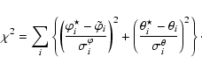
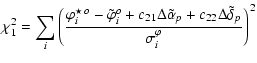
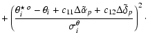
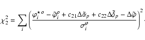
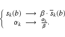
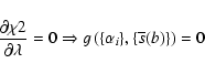
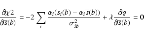
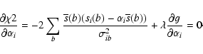
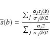

![\begin{figure}
\par\mbox{ \includegraphics[width=4.3cm, height=5cm]{5258f56.eps} \includegraphics[width=4.3cm, height=5cm]{5258f57.eps} }
\end{figure}](/articles/aa/full/2007/21/aa5258-06/img278.gif)