A&A 462, 763-767 (2007)
DOI: 10.1051/0004-6361:20066328
A. L. MacKinnon
DACE/Department of Physics and Astronomy, University of Glasgow, Glasgow G12 8QQ, UK
Received 31 August 2006 / Accepted 24 October 2006
Abstract
Aims. To quantify the solar X-ray halo resulting from inner bremsstrahlung in beta decay of neutrons generated by cosmic ray bombardment of the solar surface.
Methods. We show analytically how the angular form of this X-ray halo directly reflects the energy distribution of neutrons escaping the Sun. Previous Monte Carlo calculations of solar albedo neutron production are used to normalise an assumed parametric form for the escaping neutron distribution and thus to estimate the halo's intensity. The main remaining assumptions, that neutrons escape radially and that gravitational deceleration may be neglected, affect a negligible fraction of all solar neutrons.
Results. Observations of this halo would have clear diagnostic interest for cosmic ray propagation in the inner heliosphere. Unfortunately it is unlikely to be observable in competition with the cosmic X-ray background.
Key words: Sun: X-rays, gamma rays - plasmas - acceleration of particles
Inner bremsstrahlung (IB) is the name given to the electromagnetic radiation that accompanies beta decay of neutrons, or indeed any beta-unstable nuclei. Neutron IB was previously employed by Petrosian & Ramaty (1972) to comment on the viability of the Steady State cosmology in the light of the observed intensity of the cosmic X-ray background.
Cosmic rays impacting the solar surface will produce a quasi-static population of free neutrons surrounding the Sun (Seckel et al. 1991). This neutron population may be augmented by any ion acceleration accompanying the coronal heating process. Thus, the Sun will be surrounded by a faint, extended X-ray glow produced by IB emission as these neutrons decay. The existence of this halo should not be forgotten in discussing signatures of e.g. decaying WIMPs (Weakly Interacting, Massive Particles - Zioutas et al. 2004; DiLella & Zioutas 2003). It may also serve as a diagnostic for the ion population normally impinging on the solar surface.
The
mean lifetime of a free neutron is about 15 min. Solar neutrons around a GeV
in energy will thus extend over a region of radius ![]() 2 AU. Much more
energetic neutrons will be found throughout a greater region because of their
relativistically dilated lifetimes. Neutrons of significantly lower
energies will travel lesser distances before they decay. Thus, the angular dependence
of the intensity of this X-ray halo reflects the energy
distribution of neutrons escaping from the Sun. Its extent
distinguishes neutron IB from other cosmic ray
secondary processes (e.g. via pion production), which will be observed only
from the immediate vicinity of the solar surface.
2 AU. Much more
energetic neutrons will be found throughout a greater region because of their
relativistically dilated lifetimes. Neutrons of significantly lower
energies will travel lesser distances before they decay. Thus, the angular dependence
of the intensity of this X-ray halo reflects the energy
distribution of neutrons escaping from the Sun. Its extent
distinguishes neutron IB from other cosmic ray
secondary processes (e.g. via pion production), which will be observed only
from the immediate vicinity of the solar surface.
Properties of IB are calculated as a corollary to the Fermi theory of beta decay
(Knipp & Uhlenbeck 1936; Bloch 1936). IB radiation is more intense than the subsequent bremsstrahlung
yield of the beta-decay produced electrons - we get ![]()
![]() photons per decay, as opposed to the typically 10-5 photons per
electron slowing down in a thick target (e.g. Koch & Motz 1959). Neutrons decaying at rest
produce a very hard photon spectrum with an upper cutoff at 781 keV.
photons per decay, as opposed to the typically 10-5 photons per
electron slowing down in a thick target (e.g. Koch & Motz 1959). Neutrons decaying at rest
produce a very hard photon spectrum with an upper cutoff at 781 keV.
We describe this X-ray spectrum in more detail in Sect. 2. In Sect. 3 we show how the angular form of the IB X-ray halo reflects the energy distribution of neutrons escaping from the Sun. Section 4 leans on the previous calculation of Seckel et al. (1991) to estimate the intensity of the X-ray halo resulting from neutrons produced by cosmic rays impacting the solar surface. This halo appears not to be competitive with the cosmic X-ray background. A concluding Section considers factors that might enhance the IB flux to the level of observability and discusses further the diagnostic potential of this new component of the solar X-ray emission.
The calculation of the neutron beta decay photon spectrum, carried out by
Bloch (1936) and by Knipp & Uhlenbeck (1936), is summarised
in Petrosian & Ramaty (1972). The photon flux
goes identically to zero at 781 keV, the maximum energy of
electrons emitted in neutron beta decay. The assumptions in this theoretical
spectrum break down and it suffers
a mild infrared catastrophe as photon energy
![]() (finite energy flux, but
diverging photon number flux - Bloch 1936) but it is accurate in the X-ray photon energy range.
The photon spectrum
(finite energy flux, but
diverging photon number flux - Bloch 1936) but it is accurate in the X-ray photon energy range.
The photon spectrum
![]() (photons keV-1 neutron-1) produced by neutrons decaying at
rest is shown in Fig. 1 and
is
approximated to within 10%, for photon energies below 650 keV, by this functional form:
(photons keV-1 neutron-1) produced by neutrons decaying at
rest is shown in Fig. 1 and
is
approximated to within 10%, for photon energies below 650 keV, by this functional form:
This is a
very hard spectrum, roughly like
![]() in the
10-100 keV energy range (Fig. 1). It represents the neutron rest
frame photon spectrum, and should in principle be transformed into the
observer's frame. As long as the distribution of neutrons escaping from
the Sun declines with energy (as it does for instance in the case of the Earth, e.g. Gordon et al. 2004; Hess et al. 1959),
the majority of neutrons present along the line of sight
within 90
in the
10-100 keV energy range (Fig. 1). It represents the neutron rest
frame photon spectrum, and should in principle be transformed into the
observer's frame. As long as the distribution of neutrons escaping from
the Sun declines with energy (as it does for instance in the case of the Earth, e.g. Gordon et al. 2004; Hess et al. 1959),
the majority of neutrons present along the line of sight
within 90![]() of the Earth-Sun direction will be non-relativistic; see
Sect. 3.1 below. Thus, we may ignore this
complication for present purposes so that the photon fluence from a fixed, initial population of neutrons
is just given by the total number of neutrons
multiplied by the photon fluence
of the Earth-Sun direction will be non-relativistic; see
Sect. 3.1 below. Thus, we may ignore this
complication for present purposes so that the photon fluence from a fixed, initial population of neutrons
is just given by the total number of neutrons
multiplied by the photon fluence
![]() per neutron.
per neutron.
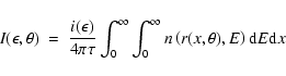
![\begin{figure}
\par\includegraphics[width=8.5cm,clip]{6328fig1.eps}
\end{figure}](/articles/aa/full/2007/05/aa6328-06/img15.gif) |
Figure 1:
Inner bremsstrahlung photon spectrum per neutron calculated numerically from the expressions
given in Petrosian & Ramaty (1972) (solid line). Also shown for comparison is the approximate fit (1) (dashed line)
but the difference between the two curves is very small in this energy range, mostly |
| Open with DEXTER | |

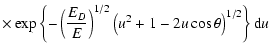
The
behaviour of the survival probability becomes more transparent for non-relativistic
neutrons. In this case it is given by
Suppose that the Sun is bombarded at a steady rate by cosmic
rays and that the resulting neutron distribution about the Sun is spherically
symmetric. Let
![]() be
the density of neutrons (cm-3) with kinetic energies between E and
be
the density of neutrons (cm-3) with kinetic energies between E and
![]() at distance r. Let the distribution at the solar surface be
at distance r. Let the distribution at the solar surface be
![]() .
We continue to assume that all neutrons move radially outward and to neglect gravitational deceleration,
discussing the consequences of these assumptions below (Sect. 4.3).
At any distance
.
We continue to assume that all neutrons move radially outward and to neglect gravitational deceleration,
discussing the consequences of these assumptions below (Sect. 4.3).
At any distance
![]() ,
n is given by
,
n is given by
![\begin{figure}
\par\includegraphics[width=6.5cm,clip]{6328fig2.eps}
\end{figure}](/articles/aa/full/2007/05/aa6328-06/img32.gif) |
Figure 2: Geometry for calculation of X-ray halo brightness as a function of angle to the Earth-Sun direction. |
| Open with DEXTER | |
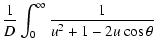
Immediately, we see that the IB spectrum at Earth
![]() (photons keV-1 s-1 cm-2 sterad-1), at photon energy
(photons keV-1 s-1 cm-2 sterad-1), at photon energy ![]() and angle
and angle ![]() to the Earth-Sun distance (Fig. 2) is
to the Earth-Sun distance (Fig. 2) is
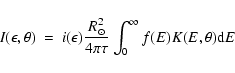
Using (3) in (4) we rewrite this in terms of f(E):
The observed photon spectrum
![]() will be separable in
will be separable in ![]() and
and ![]() .
Its
.
Its
![]() -dependence is determined by an integral over the neutron energy
distribution f(E) at the Sun. Measurements of this
-dependence is determined by an integral over the neutron energy
distribution f(E) at the Sun. Measurements of this ![]() -dependence might
allow us to deduce f(E) via the usual regularization techniques
(e.g. Craig & Brown 1986) applied to Eqs. (6) and (7), or
via forward fitting of parametric models. In turn, then, we might
comment on the energy distribution of cosmic rays arriving at the Sun and
their transport in the solar atmosphere.
-dependence might
allow us to deduce f(E) via the usual regularization techniques
(e.g. Craig & Brown 1986) applied to Eqs. (6) and (7), or
via forward fitting of parametric models. In turn, then, we might
comment on the energy distribution of cosmic rays arriving at the Sun and
their transport in the solar atmosphere.
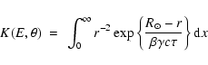
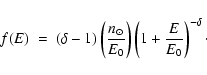
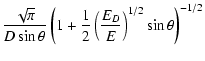
Some further analytical development is possible, which might aid in the
application of standard numerical techniques. In the Appendix we give an approximate
form for
![]() ,
valid roughly for
,
valid roughly for
![]() .
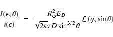
Using this
in (6) we find
.
Using this
in (6) we find
Calculations of escaping neutron distributions in flares (e.g. Hua & Lingenfelter 1987; Hua et al. 2002) have certain characteristic features. At energies of 10s of MeV and above, the neutron energy distribution mirrors the incident, primary ion energy distribution. At lower energies it becomes almost energy-independent, dominated by the scattering and thermalisation processes inevitably implicated in neutron escape from the Sun, as well as by the behaviour of the production cross-sections near threshold.
Thus, the energy distribution of escaping neutrons may be modelled with
the functional form
Terrestrial atmospheric neutrons measured at sea level or at high altitude (Hess et al. 1959) offer another guide to the possible form of the solar neutron energy distribution, albeit one dominated by cosmic ray interaction with heavier species. This distribution is harder in the >100 MeV energy range than our form (9) but steepens again below about 20 MeV (Gordon et al. 2004). Below we also comment on the consequences of adopting this distribution as a guide.
We can use the predicted neutron flux from Seckel et al. (1991) and the guessed
energy distribution (9) to estimate the neutron density near
the Sun. First of all we fix ![]() by requiring that Eqs. (3)
and (9) together imply the same flux at 1 AU of >100 MeV
neutrons predicted by Seckel et al. (1991). We find
by requiring that Eqs. (3)
and (9) together imply the same flux at 1 AU of >100 MeV
neutrons predicted by Seckel et al. (1991). We find
![]() cm-3.
cm-3.
We can now make some preliminary rough estimates of the form and intensity of the
neutron IB halo. Neutron numbers fall off rapidly above E0 = 10 MeV,
while lower energy neutrons decay closer to the Sun.
Thus, the characteristic size of the IB halo
will be given by the distance travelled by 10 MeV neutrons in a time ![]() ,
about
,
about
![]() .
The angular radius of the halo will be
.
The angular radius of the halo will be
As a more precise illustration, Fig. 3 shows the angular part of the
IB X-ray flux as a function of angle ![]() to the
Earth-Sun direction, using
to the
Earth-Sun direction, using
![]() ,
E0 = 10 MeV and fixing
,
E0 = 10 MeV and fixing ![]() as above.
Values shown in this figure need only be multiplied by the value
of
as above.
Values shown in this figure need only be multiplied by the value
of
![]() at a particular value of
at a particular value of ![]() ,
or its integral over a
given photon energy range, to yield a photon flux
,
or its integral over a
given photon energy range, to yield a photon flux
![]() (photons cm-2 keV-1 sterad-1 s-1).
(photons cm-2 keV-1 sterad-1 s-1).
Figure 3 was calculated using the exact expressions (6) and (7).
Apart from the adoption of the energy distribution (9), the main assumptions are
that all neutrons travel radially, and that gravitational deceleration may be neglected. The former
assumption minimises neutron travel times to any given location, and thus sets an upper limit
on the IB flux from any direction. Its relaxation will be most important for neutrons that travel ![]() or less in a time
comparable to
or less in a time
comparable to ![]() ,
i.e. for neutron energies of about 4 keV or less. As already mentioned, neutrons of 2 keV or less do not
actually escape so these will be present near the Sun in greater numbers than estimated here.
10 keV is thus a rough upper limit to the neutron energy at which both these effects become important. With the
form (9), such neutrons amount to just 0.2% of the total population. A different assumption about the
angular distribution of neutrons would affect Fig. 3 negligibly, as would the gravitational trapping of low energy
neutrons near the Sun.
,
i.e. for neutron energies of about 4 keV or less. As already mentioned, neutrons of 2 keV or less do not
actually escape so these will be present near the Sun in greater numbers than estimated here.
10 keV is thus a rough upper limit to the neutron energy at which both these effects become important. With the
form (9), such neutrons amount to just 0.2% of the total population. A different assumption about the
angular distribution of neutrons would affect Fig. 3 negligibly, as would the gravitational trapping of low energy
neutrons near the Sun.
Gordon et al. (2004) give an analytical expression, valid in the range 0.1-10 000 MeV, representing their experimentally measured results for the
terrestrial neutron energy distribution. We repeated the above exercise
using this energy distribution. The X-ray flux then falls off much more
steeply with angle than shown in Fig. 3, dropping by an order of magnitude in just 2![]() .
This is because this distribution continues to increase to lower neutron energies, as
opposed to the energy-independence characterising the low-energy behaviour of (9). However, the
terrestrial neutron distribution is much flatter in the 10-100 MeV range than (9),
especially with
.
This is because this distribution continues to increase to lower neutron energies, as
opposed to the energy-independence characterising the low-energy behaviour of (9). However, the
terrestrial neutron distribution is much flatter in the 10-100 MeV range than (9),
especially with
![]() ,
so total numbers, fixed by the Seckel et al. 1 AU result, are much smaller and
the peak intensity of the X-ray halo is smaller by two orders of magnitude.
,
so total numbers, fixed by the Seckel et al. 1 AU result, are much smaller and
the peak intensity of the X-ray halo is smaller by two orders of magnitude.
![\begin{figure}
\par\includegraphics[width=8.5cm,clip]{6328fig3.eps}
\end{figure}](/articles/aa/full/2007/05/aa6328-06/img61.gif) |
Figure 3:
|
| Open with DEXTER | |
We must compare this predicted X-ray flux with the general (cosmic) X-ray background flux
which has a value of
![]() erg s-1 cm-2 deg-2 integrated
over the 2-10 keV photon energy range (Moretti et al. 2003; McCammon & Sanders 1990).
To
compare the Sun's IB halo with this value, we simply multiply
the values in Fig. 3 by
erg s-1 cm-2 deg-2 integrated
over the 2-10 keV photon energy range (Moretti et al. 2003; McCammon & Sanders 1990).
To
compare the Sun's IB halo with this value, we simply multiply
the values in Fig. 3 by
 |
(10) |
The Sun's IB halo, a previously undiscussed component of solar X-radiation, posesses significant potential as a diagnostic of the fast ion distribution impinging on the solar surface. As we have seen here, its angular form directly reflects the energy distribution of neutrons escaping from the Sun. Our estimate of its intensity suggests it will be too faint to observe, however, at least if produced only by cosmic rays. We list some factors that might work in the direction of optimism.
First, any Quiet Sun ion acceleration, possibly entailed in the coronal heating process, will enhance the escaping neutron population and the IB halo intensity. We have to note the existence of observational upper limits to the Quiet Sun photon flux in the 2.223 MeV neutron capture line, ruling out >10 MeV ions as a major energy transport mechanism in coronal heating (Harris et al. 1992) and incidentally placing limits on the likely Quiet Sun neutron population.
The work of Seckel et al. (1991) plays a central role in the estimate of IB intensity so we should note some of its assumptions. It employs a specific model for small-scale magnetic fields which should be re-examined, particularly since potential extrapolations from magnetogram data are now available routinely (e.g. Schrijver & DeRosa 2003). At solar minimum, as the Sun's magnetic polarity reverses, there may be times when cosmic rays arrive much more easily at the solar surface (see Moraal et al. 2005) and the escaping neutron population would be temporarily enhanced at these times. Seckel et al. neglect incident and target species heavier than 4He, even although these can make a non-negligible contribution to neutron production in flares (Hua & Lingenfelter 1987; Hua et al. 2002). We note that the updated treatment of reaction kinematics used in Hua et al. (2002) accounts for a 50% increase in neutron yields over the earlier treatment of Hua & Lingenfelter (1987).
Adopting the terrestrial neutron energy distribution as an alternative to (9) resulted in a much fainter X-ray halo, fading much more rapidly with angle from the solar direction. Measurements (Gordon et al. 2004) represent the neutron energy distribution within the terrestrial atmosphere, not the distribution of escaping neutrons. In the flare calculations of Hua et al. (2002), few lower energy, multiply scattered neutrons escape. The assumptions made there about the propagation of accelerated ions in flare loops may not be correct for discussing the impact of galactic cosmic rays on the solar surface, however. Together with the factors mentioned in the previous paragraph, this highlights the need for further calculations of cosmic ray neutron production in the spirit of Seckel et al. (1991), concentrating particularly on the angular and energy distribution of lower energy neutrons near the Sun.
Seckel et al. (1991) commented that the neutron flux at Earth following a flare was many orders of magnitude greater than their predicted, cosmic-ray produced neutron flux. The neutrons escaping into space following a flare (Chupp et al. 1987) will also radiate via IB, though the angular distribution of this radiation will have a rapidly time-varying form of quite different significance to that discussed here. A preliminary estimate suggests that the neutrons accompanying a large flare, e.g. as described by Chupp et al. (1987) will produce an IB photon flux comparable with the background signal experienced in the RHESSI (Lin et al. 2002) mission, thus potentially close to observable. This component of flare X-radiation will be discussed elsewhere.
Finally we note that neutron detectors planned for inner heliosphere space missions (e.g. Bravar et al. 2005) should be able to directly detect the quasi-static escaping neutron population: the very modest density found in Sect. 4.3 still corresponds to a flux near the Sun of order 1 neutron cm-2 s-1. Even if IB X-radiation proves unobservable from 1 AU, the diagnostic possibilities of this neutron population, directly detected, should still be exploitable.
Acknowledgements
I first learnt about inner bremsstrahlung from the late Reuven Ramaty, as a summer visitor to NASA Goddard Space Flight Center in 1984. I thank Hugh Hudson for useful comments and discussions. The referee, Brian Dennis, also made helpful comments. Solar physics research in Glasgow is supported by a PPARC Rolling Grant. This research has made use of NASA's Astrophysics Data System.