A&A 459, 1-19 (2006)
DOI: 10.1051/0004-6361:20053898
Supersonic turbulence in shock-bound interaction zones
I. Symmetric settings
D. Folini1 - R. Walder2,3
1 - Institut für Astronomie, ETH Zürich, 8092 Zürich,
Switzerland
2 -
Observatoire de Strasbourg,
67000 Strasbourg, France
3 -
Max-Planck-Institut für Astrophysik, 85741 Garching, Germany
Received 24 July 2005 / Accepted 26 June 2006
Abstract
Colliding hypersonic flows play a decisive role in many astrophysical
objects. They contribute, for example, to the molecular cloud structure, the
X-ray emission of O-stars, differentiation of galactic sheets, appearance of
wind-driven structures, or, possibly, to the prompt emission of  -ray
bursts. Our intention is thorough investigation of the turbulent interaction
zone of such flows, the cold dense layer (CDL). In this paper, we focus on
the idealized model of a 2D plane parallel isothermal slab and on symmetric
settings, where both flows have equal parameters. We performed a set of
high-resolution simulations with upwind Mach-numbers,
-ray
bursts. Our intention is thorough investigation of the turbulent interaction
zone of such flows, the cold dense layer (CDL). In this paper, we focus on
the idealized model of a 2D plane parallel isothermal slab and on symmetric
settings, where both flows have equal parameters. We performed a set of
high-resolution simulations with upwind Mach-numbers,
 .
We find that the CDL is irregularly shaped and has a patchy and filamentary
interior. The size of these structures increases with
.
We find that the CDL is irregularly shaped and has a patchy and filamentary
interior. The size of these structures increases with
 ,
the extension of the CDL. On average, but not at each moment, the solution
is nearly self-similar and only depends on
,
the extension of the CDL. On average, but not at each moment, the solution
is nearly self-similar and only depends on
 .
We give the
corresponding analytical expressions, with numerical constants derived from
the simulation results. In particular, we find the root-mean-square
Mach-number to scale as
.
We give the
corresponding analytical expressions, with numerical constants derived from
the simulation results. In particular, we find the root-mean-square
Mach-number to scale as
 .
The
mean density,
.
The
mean density,
 is
independent of
.
The fraction
is
independent of
.
The fraction
 of the
upwind kinetic energy that survives shock passage scales as
of the
upwind kinetic energy that survives shock passage scales as
 .
This dependence persists if
the upwind flow parameters differ from one side to the other of the CDL,
indicating that the turbulence within the CDL and its driving are mutually
coupled. Another finding points in the same direction, namely that the
auto-correlation length of the confining shocks and the characteristic
length scale of the turbulence within the CDL are proportional. Larger
upstream Mach-numbers lead to a faster expanding CDL, confining interfaces
that are less inclined with respect to the upstream flow direction, more
efficient driving, and finer interior structure with respect to the
extension of the CDL.
.
This dependence persists if
the upwind flow parameters differ from one side to the other of the CDL,
indicating that the turbulence within the CDL and its driving are mutually
coupled. Another finding points in the same direction, namely that the
auto-correlation length of the confining shocks and the characteristic
length scale of the turbulence within the CDL are proportional. Larger
upstream Mach-numbers lead to a faster expanding CDL, confining interfaces
that are less inclined with respect to the upstream flow direction, more
efficient driving, and finer interior structure with respect to the
extension of the CDL.
Key words: shock waves - instabilities - turbulence
- hydrodynamics - ISM: kinematics and dynamics - stars: winds, outflows
1 Introduction
Supersonically turbulent, shock-bound interaction zones are important
for a variety of astrophysical objects. They contribute, for example,
to structure formation in molecular clouds (Ballesteros-Paredes et al. 1999a; Heyer & Brunt 2004; Vázquez-Semadeni 2004; Hartmann et al. 2001; Hueckstaedt 2003; Hunter et al. 1986) and to galaxy
formation (Kang et al. 2005; Anninos & Norman 1996). They affect the
X-ray emission of line-driven hot-star winds (Feldmeier & Owocki 1998; Feldmeier et al. 1997; Oskinova et al. 2004; Owocki et al. 1988) and
contribute substantially to the physics and emitted spectrum of
colliding wind binaries (Stevens et al. 1992; Marchenko et al. 2003; Corcoran et al. 2005; Folini & Walder 2000; Nussbaumer & Walder 1993). The
currently most promising model for the prompt emission of -ray
bursts is based on internal shocks (Fan & Wei 2004; Piran 2004; Panaitescu et al. 1999; Rees & Meszaros 1994). A similar mechanism
has been proposed for micro-quasars (Kaiser et al. 2000), BL Lacs
and Blazars (Mimica et al. 2004; Ghisellini et al. 2002), and
Herbig-Haro objects (Matzner & McKee 1999).
So far, the shape and turbulent interior of shock-bound interaction zones have
been mostly studied separately. In this paper we focus on the system as a
whole, stressing that upwind flows, confining interfaces of the interaction
zone, and the interior structure of this zone form a tightly coupled system.
The turbulence within the interaction zone affects the shape of the confining
shocks, which in turn determines how much energy is thermalized at these
shocks and how much energy remains available for driving the turbulence.
A variety of papers have been written on the shape and stability of 2D interaction zones, of which we mention only a few. Vishniac (1994) shows
by analytical means that geometrically thin, isothermal, 2D, planar,
shock-bounded slabs are non-linearly unstable, coining the term non-linear
thin shell instability, or NTSI, for this instability.
Blondin & Marks (1996) essentially reproduce these analytical predictions
numerically, also mentioning the occurrence of supersonic turbulence within
the slab. Performing 2D radiative and isothermal simulations of colliding
molecular clouds, Klein et al. (1998) observe the complex shaping and
instability of the collision zone. The role of a radiative cooling layer has
been addressed by several authors. Strickland & Blondin (1995) numerically
investigated flows against a wall in 2D, finding that an unstable cooling
layer introduces disturbances in the interface separating the cooling layer
from the cooled matter. Looking at colliding flows instead of a flow against
a wall, Walder & Folini (1998) show that one unstable cooling layer is
sufficient to destabilize both confining interfaces of the cooled matter. In
addition, the cooled matter becomes supersonically turbulent. If self-gravity
is included fragmentation of the interaction zone is observed
(Anninos & Norman 1996; Hunter et al. 1986).
An overwhelming amount of literature meanwhile exists on supersonic
turbulence. At least part of this attention arises because it is thought that
supersonic turbulence can explain the structuring and support of molecular
clouds and thus that it plays a decisive role in star formation. A
comprehensive view of this issue can be found in the recent reviews
by Mac Low & Klessen (2004), Elmegreen & Scalo (2004)
and Scalo & Elmegreen (2004). Of particular interest for the work we present
here is the paper by Mac Low (1999), where Fig. 4 shows that the
wave length of the driving is apparent in the spatial scale of the turbulent
structure for monochromatically driven turbulence in a 3D periodic box. The
possible importance of the finite size of the slab was recently pointed out by
Burkert & Hartmann (2004).
We are trying to make four points with this paper. First, we argue that,
within the frame of isothermal Euler equations and in infinite space, the
solution may be self-similar and dependent only on the upstream Mach-number,
at least to first approximation. Based on this assumption, we give expressions
for average quantities of the slab. Second, we show that the numerical
solution, which is defined only on a finite computational domain and includes
(implicit) numerical dissipation, remains close to self-similar, as long as the
width of the slab is small and the root-mean-square Mach-number larger than
one. Third, we stress the tight mutual coupling between the turbulence and
its driving. Fourth, we point out that spatial scales generally grow with
extension
of the interaction zone, but decrease with
increasing upstream Mach-number
.
Results are based on a set of simulations that differ only in their upwind
Mach-numbers. In this paper we restrict the analysis of these simulations to
the above-mentioned three objectives. We postpone a more detailed analysis of
the interior structure of the interaction zone to a subsequent paper.
In the following, we first give the details of our physical model and
numerical method in Sect. 2. In
Sect. 3 we derive the self-similar scaling relations. The
numerical results are present in Sect. 4. Discussion
follows in Sect. 5, and conclusions in
Sect. 6.
2 Physical model and numerical method
The numerical treatment of supersonic turbulence is an issue in its
own right, so we start this section with a brief summary of some
results that are relevant to the present work. We then specify the
physical model we consider, explain the numerical method we use and
the simulations we perform.
2.1 Simulating supersonic turbulence
The shock-compressed layer studied in this paper is supersonically turbulent
with root-mean-square Mach-numbers between about 1 and 10. An important
fraction of the kinetic energy is dissipated in shocks. Euler equations are
sufficient for describing this part of the problem. A cascade transfers the
remaining energy to higher and higher wave numbers until it is finally
destroyed on the viscous dissipation scale. To also capture this part of the
problem, the compressible Navier-Stokes equations should be used; however,
the range of spatial scales associated with the energy cascade exceeds the
capacity of any computer by far.
In subsonic turbulence, one way out is to use a suitable sub-grid scale model.
The model is used to compute an effective viscosity coefficient, which should
mimic the cascading between the smallest scale still resolved by the numerical
grid and the viscous dissipation scale as precisely as possible. This
coefficient is then used in the Navier-Stokes equations instead of the
physical viscosity (Lesieur 1999). For the approach to work it
is essential that the effective viscosity obtained from the sub-grid scale
model exceeds the (implicit) numerical viscosity of the overall numerical
scheme. This can be achieved in subsonic turbulence by the use of
low-dissipation schemes (Lele 1992).
In supersonic turbulence, explicit sub-grid scale modeling so far does not
exist in the above sense. The basic reason is that the numerical treatment of
supersonic turbulence requires schemes that can treat shocks appropriately,
such as the widely used shock capturing schemes. The (implicit) numerical
viscosity of such schemes is, however, much too large to match the above
requirement, even if the schemes are of a high order (Garnier et al. 1999; Porter et al. 1992). One strategy for this case, the so called MILES approach
(monotone integrated large-eddy simulation), was proposed
by Boris et al. (1992) and further explored
by Porter et al. (1994,1992). The basic claim is that the
numerical viscosity inherent to shock capturing schemes (LeVeque 2002; Hirsch 1995) acts already as a physically correct sub-grid scale model.
Solving the Euler equations by means of a shock capturing scheme thus should
yield the correct physical answer.
The validity of the claim that implicit numerical viscosity alone leads to a
correct physical solution was investigated by Garnier et al. (1999) for a
selection of shock capturing schemes, among them a MUSCL-scheme (monotone
upwind scheme for conservation laws) similar to the one we use (see
Sect. 2.3). For the cases considered (essentially decaying
subsonic), they find that the scheme indeed acts as a (very dissipative)
sub-grid scale model in that it preserves the flow from energy accumulation on
small spatial scales. However, they also find that structures defined on less
than 5 grid points are affected by substantial numerical damping.
Porter et al. (1994) find, in addition, that the dissipation properties of
their scheme (MUSCL with PPM) are highly non-linear, and also they depend not
only on the grid spacing but also on the wave length of the flow structure.
Structures on less than 32 grid points are affected by numerical damping.
We rely on the MILES approach in this paper for the lack of a better model,
although, to our knowledge, the validity and quality of the approach has never
been tested for supersonic turbulence. The numerical solutions we obtain are
thus rather solutions of the Navier-Stokes equations. Nevertheless, as
dissipation in shocks by far dominates numerical dissipation, we expect the
"Euler character'' of the solution to prevail.
2.2 The model problem
The model problem we consider consists of a 2D, plane-parallel, infinitely
extended, isothermal, shock compressed slab. A sketch is given in
Fig. 1. Two high Mach-number flows, oriented parallel (left
flow, subscript l) and anti-parallel (right flow, subscript r) to the
x-direction, collide head on. The resulting high-density interaction zone, the
shock compressed slab, is oriented in the y-direction. We denote this
interaction zone by CDL for "cold dense layer'' to remain consistent with
notation used already in Walder & Folini (1998,1996). We
investigated this system within the frame of Euler equations (but see also
Sect. 2.1), together with a polytropic equation of state,
 |
= |
0, |
(1) |
 |
= |
0, |
(2) |
 |
= |
0, |
(3) |
| e |
= |
 |
(4) |
Here,  is the particle density,
  the average mass per particle,
 is the velocity vector, p thermal
pressure, I the identity tensor, e the thermal energy density, and
is the velocity vector, p thermal
pressure, I the identity tensor, e the thermal energy density, and
 the total energy density. For the polytropic exponent, we
choose
the total energy density. For the polytropic exponent, we
choose
 .
This value guarantees that jump conditions and
wave speeds of a Mach-90 shock are within 0.01 per cent of the isothermal
values.
.
This value guarantees that jump conditions and
wave speeds of a Mach-90 shock are within 0.01 per cent of the isothermal
values.
Within the frame of this paper we consider only symmetric settings,
where the left (subscript l) and right (subscript r) colliding
flow have identical parameters (subscript u for upstream):
 and
and
 .
.
We look at the problem in a dimensionless form and express velocities in units
of the isothermal sound speed
 ,
with T the
temperature and
,
with T the
temperature and
 the Boltzmann constant. Densities we express
in terms of the upstream density
the Boltzmann constant. Densities we express
in terms of the upstream density
 .
Finally, we express
lengths in units of
.
Finally, we express
lengths in units of
 ,
the smallest y-extent of the
computational domain we used. This artificial choice is necessary as
there is no natural time-independent length scale to the problem (see
Sect. 3).
,
the smallest y-extent of the
computational domain we used. This artificial choice is necessary as
there is no natural time-independent length scale to the problem (see
Sect. 3).
![\begin{figure}
\par\includegraphics[width=8.8cm,clip]{3898f1.eps}\end{figure}](/articles/aa/full/2006/43/aa3898-05/Timg89.gif) |
Figure 1:
Sketch of physical model problem.
 ,
Mi, and si denote the density, Mach-number, and
confining shock of the left ( ,
Mi, and si denote the density, Mach-number, and
confining shock of the left ( )
and right ( )
and right ( )
flow.
and M denote the density and Mach-number of the CDL. )
flow.
and M denote the density and Mach-number of the CDL.  is the absolute
value of the angle between the x-axis and the tangent to the shock. CDL is
the shock-compressed interaction zone. The dashed rectangle indicates the
computational domain with y-extension Y. Periodic boundary conditions in
y-direction imply periodic continuation of the solution (dotted continuation
of left and right shock).
is the absolute
value of the angle between the x-axis and the tangent to the shock. CDL is
the shock-compressed interaction zone. The dashed rectangle indicates the
computational domain with y-extension Y. Periodic boundary conditions in
y-direction imply periodic continuation of the solution (dotted continuation
of left and right shock). |
| Open with DEXTER |
2.3 Numerical method
Our results were obtained with the AMRCART-code![[*]](/icons/foot_motif.gif) . We used
the multidimensional high-resolution finite-volume-integration scheme
developed by Colella (1990) on the basis of a Cartesian mesh.
Tests showed that this algorithm, compared to dimensional splitting
schemes, is significantly more accurate in capturing flow features not
aligned with the axis of the mesh. In all our simulations we used a
version of the scheme that is (formally) second order accurate in
space and in time for smooth flows.
. We used
the multidimensional high-resolution finite-volume-integration scheme
developed by Colella (1990) on the basis of a Cartesian mesh.
Tests showed that this algorithm, compared to dimensional splitting
schemes, is significantly more accurate in capturing flow features not
aligned with the axis of the mesh. In all our simulations we used a
version of the scheme that is (formally) second order accurate in
space and in time for smooth flows.
We combine this integration scheme with the adaptive mesh algorithm
by Berger (1985). While a rather coarse mesh was sufficient for the upwind
flows, the turbulent CDL was resolved on a much finer scale.
We found it useful to have our CDL moving in positive x-direction at a speed
of about Mach 20-40. If the CDL was essentially stationary with respect to the
computational grid, we observed alignment effects of strong shocks that were
nearly parallel to a cell interface (in y-direction). Through the global
motion of the CDL, which implied supersonic motion of the confining shocks
with respect to the computational grid, we got rid of this problem. We
checked that this procedure introduced no systematic effects into the
solution. The problem of alignment effects when dealing with high Mach-number
flows, nearly stationary shocks, and high order upwind schemes is well known
and not particular to our scheme (Jasak & Weller 1995; Colella & Woodward 1984; Quirk 1994). Other work arounds exist, such as smoothing of interfaces
by additional viscosity, which is often applied in PPM implementations.
2.3.1 Numerical settings and integration time
In the x-direction, our computational domain extended over
 .
The y-extent Y of our domain
varied between simulations,
.
The y-extent Y of our domain
varied between simulations,
 (see Table B.1).
Boundary conditions at the left and right boundaries (x-direction) were
"supersonic inflow''. In the y-direction we had periodic boundary
conditions. The cell size at the coarsest level was
(see Table B.1).
Boundary conditions at the left and right boundaries (x-direction) were
"supersonic inflow''. In the y-direction we had periodic boundary
conditions. The cell size at the coarsest level was
 .
The cells at the finest level, covering the
CDL, were smaller by a factor 26 to 29, yielding between 320 and 2560 cells over a distance
(depending
on the simulation, see Table B.1).
.
The cells at the finest level, covering the
CDL, were smaller by a factor 26 to 29, yielding between 320 and 2560 cells over a distance
(depending
on the simulation, see Table B.1).
As will be shown, the relevant time-dependent quantity for the
evolution of CDL mean quantities is the average x-extension of the
CDL,
.
We defined it as
 ,
where V is the 2D volume of the CDL. For
later use we also introduce the volume integrated density
,
where V is the 2D volume of the CDL. For
later use we also introduce the volume integrated density
 ,
the mean density
,
the mean density
 ,
and the average
column density
,
and the average
column density
 .
The last quantity was made
dimensionless by division through
.
The last quantity was made
dimensionless by division through
 .
We stopped most simulations
at
.
We stopped most simulations
at
 .
.
2.3.2 Initial conditions
We investigated three different initial conditions, I=0, 1, 2.
I=0: No CDL exists at t=0. The left and right flows are
initially separated by a single interface. The interface is wiggled
with a single, sinusoidal mode of wave length 0.1 Y and amplitude
 (about 3 to 25 grid cells, depending on the
discretization).
(about 3 to 25 grid cells, depending on the
discretization).
I=1: A CDL is present at time t=0. It has a column density of
 and a thickness of
 .
The confining shocks are both wiggled, with
the same sinusoidal mode and amplitude as the interface in the case
I=0. The mass within the CDL is at rest and of constant density,
.
The confining shocks are both wiggled, with
the same sinusoidal mode and amplitude as the interface in the case
I=0. The mass within the CDL is at rest and of constant density,
 ,
the density the CDL would
have in 1D. Note that this initialization implies some violation of
the Rankine-Hugoniot jump conditions at the interfaces.
,
the density the CDL would
have in 1D. Note that this initialization implies some violation of
the Rankine-Hugoniot jump conditions at the interfaces.
I=2: A CDL is present at time t=0, with column density
 and a thickness of
 .
The right shock is wiggled as for I=1, the
left shock is straight. The density and velocity in the CDL are set as
for I=1.
.
The right shock is wiggled as for I=1, the
left shock is straight. The density and velocity in the CDL are set as
for I=1.
We stress that the initial wiggling of the shocks is not compelling. The only
effect of this wiggling is to speed up the initial phase of the evolution.
Test cases using another wiggling or starting from straight shocks end up like
the simulations we are going to present in the following.
We would like to add a side note on this last point, from our observation that
the slab is also destabilized when bound by straight shocks. This has already
been reported by Blondin & Marks (1996), who ascribed the destabilization to
"numerical noise''. Meanwhile, Robinet et al. (2000) have investigated what
is called the carbuncle phenomenon in some more detail. They showed that -
contrary to what has been believed so far - a single straight shock is linearly
unstable for exactly one mode associated to the upstream Mach-number of
![$M_{{\rm crit}} = [(5+\gamma) / (3-\gamma)]^{1/2}$](/articles/aa/full/2006/43/aa3898-05/img105.gif) .
For isothermal
conditions, this yields
.
For isothermal
conditions, this yields
 .
They also showed that
this single unstable mode is sufficient for making straight shocks aligned with
the mesh numerically unstable at all Mach-numbers if the computation is done
with a low-viscosity, high-order, shock-capturing scheme. To what degree this
instability for a straight shock of any Mach-number is really physical seems
an open question to us.
.
They also showed that
this single unstable mode is sufficient for making straight shocks aligned with
the mesh numerically unstable at all Mach-numbers if the computation is done
with a low-viscosity, high-order, shock-capturing scheme. To what degree this
instability for a straight shock of any Mach-number is really physical seems
an open question to us.
The runs we performed differ in their upwind Mach-numbers, which lie in a
range
 ,
as well as in their
initialization, numerical discretization, and the y-extent of the domain. The
labels of the different runs are built up as
,
as well as in their
initialization, numerical discretization, and the y-extent of the domain. The
labels of the different runs are built up as  .
Here, M is the upwind
Mach-number, I the initialization (0, 1, or 2), R gives the refinement of the
spatial discretization, relative to the coarsest grid simulation we performed
(1, 2, 4, or 8). R=1 corresponds to a finest cell size of about
.
Here, M is the upwind
Mach-number, I the initialization (0, 1, or 2), R gives the refinement of the
spatial discretization, relative to the coarsest grid simulation we performed
(1, 2, 4, or 8). R=1 corresponds to a finest cell size of about
 ,
R=2 indicates a twice smaller cell size.
Y is the domain size (1, 2, 4, or 6) in units of
.
For example, R22_0.2.4 denotes a run with
,
R=2 indicates a twice smaller cell size.
Y is the domain size (1, 2, 4, or 6) in units of
.
For example, R22_0.2.4 denotes a run with
 ,
initialization
I=0, finest cell size about
,
initialization
I=0, finest cell size about
 ,
and
y-extent
,
and
y-extent
 .
.
The runs we performed are listed in Table B.1. Individual
columns in Table B.1 contain (column number in square
brackets): label of run [1], following the scheme
label=
 ,
where I is the initial condition, R the
refinement factor such that cell size =
,
where I is the initial condition, R the
refinement factor such that cell size =
 ,
and Y is the y-extension of the
computational domain in units of
;
Mach-number of
upstream flow,
[2]; stopping time of simulation in terms of
,
and Y is the y-extension of the
computational domain in units of
;
Mach-number of
upstream flow,
[2]; stopping time of simulation in terms of  [3]; y-averaged x-extension of CDL at stopping time, relative to y-extent of computational domain,
 [4];
average quantities [5-8] of: rms Mach-number,
[4];
average quantities [5-8] of: rms Mach-number,
 [5]; mean
density in units of upstream density,
[5]; mean
density in units of upstream density,
 [6]; shock length in units of y-domain,
 [7]; driving
efficiency,
[8]; averages taken over
[7]; driving
efficiency,
[8]; averages taken over
 for I=0 and over
 for I=1, for I=2 we give the
values at the end of the simulation in parentheses instead.
for I=1, for I=2 we give the
values at the end of the simulation in parentheses instead.
3 Scaling properties of the model problem
![\begin{figure}
\par\includegraphics[width=6cm,clip]{3898f2a.eps}\par\vspace*{2mm}
\includegraphics[width=6cm,clip]{3898f2b.eps}
\end{figure}](/articles/aa/full/2006/43/aa3898-05/Timg118.gif) |
Figure 2:
The self-similar 1D solution of isothermal colliding supersonic flows
in density ( top) and velocity ( bottom). The interaction zone
(labeled CDL) is bounded by two shocks,
 and
and
 ,
having speeds ,
having speeds
 and
and
 in the rest
frame of the CDL. The density and velocity of the 1D interaction zone,
we denote by
in the rest
frame of the CDL. The density and velocity of the 1D interaction zone,
we denote by
 and
and
 ,
respectively. ,
respectively. |
| Open with DEXTER |
Within the frame of Euler equations and in infinite space, the problem of
isothermal supersonically colliding flows can be solved analytically in 1D.
The solution, sketched in Fig. 2 and
Sect. 3.1, is self-similar and depends only on two free
parameters, the Mach-numbers of the left and right upwind flow. In 2D the
situation is more complicated: the solution is unstable (Blondin & Marks 1996; Vishniac 1994), the shocks confining the CDL are non-stationary and
oblique, the interior of the CDL is supersonically turbulent.
Nevertheless, in infinite space it seems reasonable to assume
that the solution, on average, may still evolve in a self-similar
manner. We base this assumption on the following two observations.
First, the isothermal Euler equations are scale-free in infinite
space. Second, the free parameters of the problem
(
,
,
and a) do not introduce any
fixed length or time scale. Under these conditions, it is possible
that the solution also does not depend on length or time separately,
but only on their ratio. If so, all length scales should evolve
equally with time, which implies, in particular, that the solution
then should not depend on the extension of the CDL. We stress,
however, that we have no proof of the above assumption of
self-similarity.
In the remainder of this section, we elaborate a bit further on the
implications of the assumed self-similarity. In Sect. 4 we
will see that the relations derived here give a good approximation of the
numerical results, but we stress already here three important points. The
numerical simulations are carried out in finite space (not infinite);
numerical dissipation might play a role; and the simulations are stopped for
the most part while the CDL is still small, about half the size of the
y-extent of the computational domain. Important aspects that can only be
obtained from the numerical solution include quantities related to the driving
of the turbulence, the values of proportionality constants, and the interior
structure of the CDL. We neglect this last aspect, however, in the current
paper to focus on mean quantities instead.
3.1 Self-similar 1D solution
Denoting the density and velocity of the CDL by
and
,
and those of the left and right upwind flows
by
and vi ( ), the
solution in the rest frame of the CDL is given by
), the
solution in the rest frame of the CDL is given by
 |
= |
 |
(5) |
 |
= |
0, |
(6) |
| |vsi| |
= |
 |
(7) |
Here,
vsi is the velocity of the confining shocks and a is
again the isothermal sound speed. The approximations hold for large
Mach-numbers. The self-similar character is apparent: the solution is not a
function of x and t but only a function of x/t through
vsi.
A relation between characteristic length and time scales of the solution, the
self-similarity variable
 ,
can be obtained as follows.
As a length scale, we take the spatial extension
,
can be obtained as follows.
As a length scale, we take the spatial extension
 of the
CDL, and as a time scale the time
of the
CDL, and as a time scale the time  needed to accumulate the
corresponding column density
needed to accumulate the
corresponding column density
 .
From the relations
.
From the relations
 |
(8) |
and
 |
(9) |
and using
 (see Eq. (5)), we
obtain
(see Eq. (5)), we
obtain
 |
(10) |
Thus for strong shocks
is nothing else
than
 .
Specializing to
symmetric settings (
.
Specializing to
symmetric settings (
 )
yields
)
yields
 and
and
 .
.
3.2 Scaling properties of the 2D symmetric solution
In the following, we derive scaling relations for the 2D solution, assuming self-similarity. We confront these relations
with corresponding numerical results in Sect. 4.
In the following, all velocities are again given in the rest frame of
the CDL and we assume that a self-similar solution exists. A
natural choice for the (constant) self-similarity variable
then is again
 .
Using the definitions of Sect. 2.3.1 we must have, as
in the 1D case,
.
Using the definitions of Sect. 2.3.1 we must have, as
in the 1D case,
 |
|
|
(11) |
 |
|
|
(12) |
Dividing the two equations through each other yields
 .
As
.
As
 is a constant, the CDL mean density
 must be constant in time. The root-mean-square velocity
 then has to be constant in time as well, at least if
the CDL density and velocity,
and v, are uncorrelated (in which case
we can replace the average over the product
then has to be constant in time as well, at least if
the CDL density and velocity,
and v, are uncorrelated (in which case
we can replace the average over the product
 by the product of the
averages of
and v2) and if kinetic pressure dominates over thermal
pressure. This can be seen from equating the total upwind pressure with the
total pressure within the CDL,
by the product of the
averages of
and v2) and if kinetic pressure dominates over thermal
pressure. This can be seen from equating the total upwind pressure with the
total pressure within the CDL,
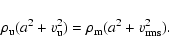 |
(13) |
The simplest ansatz for
and
 is that they only depend on the upstream Mach-number,
 |
|
|
(14) |
 |
|
|
(15) |
Using the ansatz for
we obtain a first expression for
from Eqs. (11)
and (12),
 |
(16) |
A second expression for
,
we obtain from Eq. (13)
 |
(17) |
Again using Eq. (12) to replace N, one
obtains
 |
(18) |
The approximation is good for high Mach-number flows, with
 ,
and for
,
and for
 ,
which is, however, to be expected for
supersonic turbulence. Comparing Eqs. (16)
and (18) gives
,
which is, however, to be expected for
supersonic turbulence. Comparing Eqs. (16)
and (18) gives
 |
|
|
(19) |
 |
|
|
(20) |
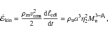
3.2.2 Driving energy
From energy conservation, we have
 .
Here
.
Here
 is the energy flux density entering the CDL per
time and per unit length in the y-direction, and
is the energy flux density entering the CDL per
time and per unit length in the y-direction, and
 denotes the energy density dissipated per time within an average
column of length
of the CDL. Finally,
denotes the energy density dissipated per time within an average
column of length
of the CDL. Finally,
 is the change per time of the kinetic energy
contained within such an average column. We first turn to the driving
energy
and come back to
and
in
Sect. 3.2.3.
is the change per time of the kinetic energy
contained within such an average column. We first turn to the driving
energy
and come back to
and
in
Sect. 3.2.3.
Part of the total (left plus right) upwind kinetic energy flux density,
 ,
is
thermalized at the shocks confining the CDL. The remaining part,
,
drives the turbulence in the CDL. We assume that
and
,
is
thermalized at the shocks confining the CDL. The remaining part,
,
drives the turbulence in the CDL. We assume that
and
 are
related by a function of the upwind Mach-number only,
are
related by a function of the upwind Mach-number only,
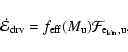 |
(21) |
We call the function
the driving efficiency. An
expression for
can be derived by using the jump
conditions for strong, oblique shocks,
The subscript d denotes downstream quantities, right after shock
passage; the subscripts
 and
and
 denote flow components perpendicular and parallel to the shock,
respectively; and
is given in Fig. 1. Using
Eq. (22) we obtain
denote flow components perpendicular and parallel to the shock,
respectively; and
is given in Fig. 1. Using
Eq. (22) we obtain
where the integral over
 and
and
 runs over both shocks and where it was used that
 .
The
last term on the right hand side of Eq. (23) is omitted in
the following. This is justified, as the shocks we observe in our simulations
fulfill
.
The
last term on the right hand side of Eq. (23) is omitted in
the following. This is justified, as the shocks we observe in our simulations
fulfill
 for the most part (see
Sect. 4.2.2). For
for the most part (see
Sect. 4.2.2). For
 we thus
obtain
we thus
obtain
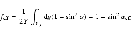 |
(24) |
where we used the midpoint rule. The angle
 can be
interpreted as an average bending angle. As the ansatz for the Mach-number
dependence of
we thus take
can be
interpreted as an average bending angle. As the ansatz for the Mach-number
dependence of
we thus take
 |
(25) |
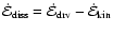
3.2.3 Energy dissipation
A first expression for the column-integrated dissipated energy per
time can be obtained from energy conservation,
.
For
we just
derived an expression, Eqs. (21) and (25).
For
we obtain, within the frame of
self-similarity,
 |
(26) |
where we used Eqs. (14), (15),
and (18) to (20). Together we get
![\begin{displaymath}\dot{\cal E}_{{\rm diss}} = \rho_{{\rm u}} a^{3} M_{{\rm u}}^...
...eta_{{\rm 2}}^{2} M_{{\rm u}}^{{\rm -\beta_{{\rm 1}}}}\right].
\end{displaymath}](/articles/aa/full/2006/43/aa3898-05/img178.gif) |
(27) |
The energy dissipated per time within an average column of length
is thus independent of this length. If
energy dissipation occurs only (as within the frame of Euler equations) or
at least dominantly in shocks, this implies that the average distance between
shocks increases and / or the average strength of the shocks decreases
as the CDL grows.
A second expression for
can be obtained
from dimensional considerations. The energy dissipated per unit volume
per unit time must be proportional to
 .
Here,
.
Here,
 ,
,
 ,
and
,
and
 are the characteristic density, velocity, and
length scale of the dissipation. The energy
dissipation within an average column of length
can thus be written as
are the characteristic density, velocity, and
length scale of the dissipation. The energy
dissipation within an average column of length
can thus be written as
 .
As all length scales must evolve equally with
time within the frame of self-similarity,
.
As all length scales must evolve equally with
time within the frame of self-similarity,
 must be constant, thus
 |
(28) |
Comparison of Eqs. (27) and (28) suggests
 and a more complicated
Mach-number dependence for
.
As
is
the only velocity scale we have, it seems natural to assume that
and a more complicated
Mach-number dependence for
.
As
is
the only velocity scale we have, it seems natural to assume that
 .
It then follows that
.
It then follows that
 or
or
 (and
(and
 ). We note that Gammie & Ostriker (1996) even found
 for a 1D case.
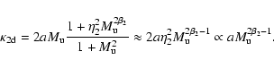
3.3 Summary of expected scaling relations
If a self-similar solution exists, we expect the following
dependencies:
 |
= |
 |
(29) |
 |
= |
 |
(30) |
 |
= |
 |
(31) |
 |
= |
 |
(32) |
 |
= |
 |
(33) |
 |
= |
 |
(34) |
Note the differences to the 1D solution: Eq. (29) predicts
the CDL mean density to be independent of
and
 ,
in contrast to
,
in contrast to
 and
and
 .
.
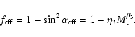
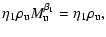
In deriving the above relations, we made four basic assumptions:
a) we have simple Mach-number dependencies of
,
,
and
,
Eqs. (14),
(15), and (25); b) the CDL density and
velocity are uncorrelated; c) we have high Mach-numbers in the sense
that
or
 ;
d)
.
;
d)
.
In Sect. 4 we are going to check the validity of these
assumptions and confront Eqs. (29) to (34) with
numerically obtained values. We expect good agreement as long as
 ,
thus dissipation in shocks likely dominates, and as
long as
,
thus dissipation in shocks likely dominates, and as
long as
 .
The "Euler character'' of the
solution should prevail under these conditions. We also determine those
quantities that cannot be derived analytically. These are, on the one hand,
the coefficients
.
The "Euler character'' of the
solution should prevail under these conditions. We also determine those
quantities that cannot be derived analytically. These are, on the one hand,
the coefficients
 and
and
 ,
as well as the
exponent
,
as well as the
exponent
 .
On the other hand, there are quantities for
which we have no analytical expression at all, like the wiggling of the
confining shocks, the associated distribution of the angle ,
or the
Mach-number dependence of the length of the confining shocks.
.
On the other hand, there are quantities for
which we have no analytical expression at all, like the wiggling of the
confining shocks, the associated distribution of the angle ,
or the
Mach-number dependence of the length of the confining shocks.
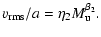
4 Numerical results
We now present our numerical results. After a brief phenomenological
description of the solution in Sect. 4.1, we give quantitative
results for initial conditions I=0 in Sect. 4.2. Results
for initial conditions I=1 and I=2 are given in
Sect. 4.3, and asymmetric settings are briefly
addressed in Sect. 4.4. Discretization and domain studies
are the topic of Sect. 4.5.
4.1 Brief phenomenological description
We begin with a brief qualitative description of the CDL. As an
example, the density structure of run R22_1.2.2 is shown in
Fig. 3 for three different times.
A first characteristic is the local bending of the confining shocks. The
spatial scale of these wiggles increases linearly with time, as the CDL
accumulates more and more matter and gets more and more extended. The
inclination of the wiggles with respect to the direction of the upstream flows
decreases with increasing upstream Mach-number (see
Sect. 4.2.2). Occasionally, we observe a superimposed "bending
mode'' (e.g. bottom panel in Fig. 3), which in
appearance is somewhat similar to the bending modes of the NTSI described
by Vishniac (1994).
A second characteristic is the patchy appearance of the CDL. The turbulent
interior is organized in filaments and patches, regions within which a flow
variable remains more or less constant. The spatial extension of these
patches increases as well as the CDL accumulates more and more matter. The
flow variables clearly mirror the supersonic character of the turbulence:
the contrast between high-density filaments and extended patches in
Fig. 3 easily reaches two orders of magnitude, the
root-mean-square velocity is well above sound, and the mean density is
substantially reduced compared to the 1D case. Shocks within the CDL are
ubiquitous.
4.2 Settings without CDL at t = 0
For symmetric settings, and if there is no CDL at time t=0, we expect to see
the self-similar relations we derived in Sect. 3.2. We
express the time evolution of the solution in terms of
 |
(35) |
This function monotonically increases at about the same rate as
the mean extension of the CDL, since
 (Eq. (29)). In fact,
 (Sect. 4.2.1) and thus
 corresponds to
 .
For the
symmetric case we consider in this paper,
is proportional
to the elapsed time. Using Eq. (12) to express N,
we can write
.
For the
symmetric case we consider in this paper,
is proportional
to the elapsed time. Using Eq. (12) to express N,
we can write
 |
(36) |
and
then corresponds to a time
 .
Or, if we use
.
Or, if we use
 (Sect. 4.2.1) and
 for
,
we obtain
for
,
we obtain
 .
.
Unless otherwise stated, averages and best fits in this section are
always taken over the interval
and over all
runs without CDL at time t=0. The interval was chosen such that
initialization effects have died away and that domain effects do not
matter yet (Sect. 4.5.1).
![\begin{figure}
\par\includegraphics[width=8.6cm,clip]{3898f3a.ps}\par\vspace{2mm...
...ps}\par\vspace{2mm}
\includegraphics[width=8.6cm,clip]{3898f3c.ps}
\end{figure}](/articles/aa/full/2006/43/aa3898-05/Timg221.gif) |
Figure 3:
The interaction zone of run R22_1.2.2, shown in density
(logarithmic scale, in units of
,
color bar from
0 to 4), for three different times:
 ( top),
 ( middle),
 ( bottom). The spatial scale of patches, filaments, and
wiggling of the confining shocks increases with .
( bottom). The spatial scale of patches, filaments, and
wiggling of the confining shocks increases with . |
| Open with DEXTER |
We mention here already that the two most extreme simulations in terms of
,
R5_0.2.4 and R87_0.2.4, often differ somewhat from the
other simulations. In the case of R5_0.2.4, we ascribe the deviation to the
only subsonic turbulence and the correlation of density and velocity
(
 and corr
 ,
see
Sect. 4.2.1). In the case of R87_0.2.4, the shocks become sometimes
too strongly inclined with respect to the computational grid to be properly
resolved by our numerical grid (Sect. 4.2.2).
,
see
Sect. 4.2.1). In the case of R87_0.2.4, the shocks become sometimes
too strongly inclined with respect to the computational grid to be properly
resolved by our numerical grid (Sect. 4.2.2).
4.2.1 CDL mean quantities and correlations
We first turn to the correlation of
and v and the CDL mean quantities
and
,
Eqs. (29)
and (30). One of our basic assumptions in deriving these
self-similar relations, namely point b) that the CDL density and velocity are
uncorrelated, we find confirmed by our simulations. For nearly all symmetric
simulations without initial CDL and for
,
we have
 .
The only exceptions are the three
low Mach-number runs R11_0.2.4, R11_0.2.2, and R5_0.2.4 with correlations
of about -0.2, -0.2, and -0.4 respectively. The top panel of
Fig. 4 shows the time evolution of corr
.
The only exceptions are the three
low Mach-number runs R11_0.2.4, R11_0.2.2, and R5_0.2.4 with correlations
of about -0.2, -0.2, and -0.4 respectively. The top panel of
Fig. 4 shows the time evolution of corr for five
selected runs that differ only in their upwind Mach-number,
for five
selected runs that differ only in their upwind Mach-number,
 .
.
In the middle and bottom panel of the the same figure,
and
 are shown as a function of
for the same runs. Two things are
apparent. First, the ratios take similar values for all five runs, indicating
that indeed
are shown as a function of
for the same runs. Two things are
apparent. First, the ratios take similar values for all five runs, indicating
that indeed
 and
and
 for the exponents in Eqs. (29) and (30). Second,
the ratios are not constant with ,
indicating that the numerical
solution is indeed only approximately self-similar. We come back to this point
in Sect. 5.
for the exponents in Eqs. (29) and (30). Second,
the ratios are not constant with ,
indicating that the numerical
solution is indeed only approximately self-similar. We come back to this point
in Sect. 5.
To determine optimum exponents
 ,
i=1,2, we rewrite
Eqs. (29) and (30) as equations for
and
,
i=1,2, we rewrite
Eqs. (29) and (30) as equations for
and
 and minimize the variance
 .
Considering all data points within
of all runs without a CDL at t=0, we find the smallest
variances for
and for
.
The
corresponding means are
.
Considering all data points within
of all runs without a CDL at t=0, we find the smallest
variances for
and for
.
The
corresponding means are
 and
and
 .
Although clearly identifiable, the
minima of
.
Although clearly identifiable, the
minima of  are relatively shallow. Changing
 or
or
 by
by  0.1, or excluding the very low Mach-number case R5_0.2.4 (for which
)
changes
by only
about 5%. By repeating the analysis but allowing for a linear dependence of
0.1, or excluding the very low Mach-number case R5_0.2.4 (for which
)
changes
by only
about 5%. By repeating the analysis but allowing for a linear dependence of
 on ,
we obtain the same optimum values for
and
but with considerably smaller
variance. As
increases from 10 to 70,
rises
by about 25% (from 25 to 31), while
decreases by about 15% (from 0.22 to 0.19).
on ,
we obtain the same optimum values for
and
but with considerably smaller
variance. As
increases from 10 to 70,
rises
by about 25% (from 25 to 31), while
decreases by about 15% (from 0.22 to 0.19).
Part of our assumption a), namely the simple Mach-number dependencies of
and
,
thus seems justified. With
 ,
assumption c),
,
assumption c),
 ,
is also fulfilled for most of our simulations. An
exception is again run R5_0.2.4, for which
,
is also fulfilled for most of our simulations. An
exception is again run R5_0.2.4, for which
 .
.
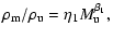
In summary, the simulation results,
 and
and
 ,
essentially confirm the expected relations, Eqs. (29)
and (30).
,
essentially confirm the expected relations, Eqs. (29)
and (30).
 ,
predicted by Eq. (20), is fulfilled to within 10% at any
given time. The mean density is (nearly) independent of
.
As expected, the solution is only approximately
self-similar,
decreases by about 15% as increases from 10 to 70.
,
predicted by Eq. (20), is fulfilled to within 10% at any
given time. The mean density is (nearly) independent of
.
As expected, the solution is only approximately
self-similar,
decreases by about 15% as increases from 10 to 70.
![\begin{figure}
\par\hspace*{-2mm}\includegraphics[width=8.9cm,clip]{3898f4a.ps}\...
...ps}\par\vspace*{2mm}
\includegraphics[width=8.7cm,clip]{3898f4c.ps}
\end{figure}](/articles/aa/full/2006/43/aa3898-05/Timg243.gif) |
Figure 4:
Time evolution of corr
( top),
( middle), and
( bottom) for runs R5_0.2.4 (dotted,
dark blue), R11_0.2.4 (dashed, purple), R22_0.2.4 (solid, red),
R33_0.2.4 (dash-dotted, orange), R43_0.2.4 (dash-three-dots,
green), and R87_0.2.4 (long dashes, pink). For these runs,
corresponds to
 . . |
| Open with DEXTER |
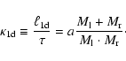
4.2.2 Confining shocks
The turbulence within the CDL is driven by the upstream flows. The confining
shocks of the CDL affect this driving in two ways. The less inclined the
shocks are on average with respect to the direction of the upstream flows
(smaller angle
in Eq. (24)), the more
kinetic energy survives shock passage and is available for driving the
turbulence. The smaller the spatial scale on which the angle
varies,
the smaller the scale on which the energy input changes. In the following, we
analyze how these shock properties depend on
and on
.
For this purpose, we specify the following basic quantities. The discrete
x-position of the left and right shocks,
and
,
defined for each discrete y-position yj as the two cell
boundaries where the Mach-number drops for the first time from its upwind
value Mu to 0.8 Mu. We determine the average extension of the CDL,
,
as
![\begin{displaymath}\ell_{{\rm cdl}} = \frac{1}{J} \sum_{j=1}^{J} [ s_{{\rm r}}(y_{j}) - s_{{\rm l}}(y_{j}) ].
\end{displaymath}](/articles/aa/full/2006/43/aa3898-05/img244.gif) |
(37) |
The length of the left and right shocks,
 and
and
 ,
are computed as
,
are computed as
![\begin{displaymath}\ell_{{\rm sh},i} = \sum_{j=1}^{J} \left[ (s_{{i}}(y_{j}) - s_{{i}}(y_{j-1}))^{2} +
(y_{j} - y_{j-1})^{2}\right]^{1/2},
\end{displaymath}](/articles/aa/full/2006/43/aa3898-05/img247.gif) |
(38) |
where J is the number of cells in y-direction, and .
We define the
angle
 as the angle between the x-axis and the
tangent to the shock (see Fig. 1). Its numerical computation
is described in Appendix A. To obtain a number distribution, we
sort the values
as the angle between the x-axis and the
tangent to the shock (see Fig. 1). Its numerical computation
is described in Appendix A. To obtain a number distribution, we
sort the values
![$\alpha_{{\rm l,r}}(y_{j}) \in [0,\pi/2]$](/articles/aa/full/2006/43/aa3898-05/img249.gif) into 60 bins.
Finally, to obtain a measure for the scale on which the shocks are wiggled, we
look at the auto-correlation functions
into 60 bins.
Finally, to obtain a measure for the scale on which the shocks are wiggled, we
look at the auto-correlation functions
 ,
,
![\begin{displaymath}\Gamma_{{i}}(y_{{\rm corr}}) = \frac{\langle[s_{{i}}(y_{j}) -...
...{\rm corr}}) - \bar{s}_{{i}}]\rangle}
{\sigma^{2}_{{\rm s}}},
\end{displaymath}](/articles/aa/full/2006/43/aa3898-05/img251.gif) |
(39) |
where
 is the variance of the shock position si, and
 denotes the mean over all discrete position yj. For each time, we determine
 such that
 .
Averaging
over both shocks
gives a mean auto-correlation length
.
Averaging
over both shocks
gives a mean auto-correlation length
 ,
,
![\begin{displaymath}\ell_{{\rm corr}} = \frac{1}{2}
\left[
y_{{\rm corr_{{\rm0...
..._{{\rm l}}) +
y_{{\rm corr_{{\rm0}}}}(s_{{\rm r}})
\right].
\end{displaymath}](/articles/aa/full/2006/43/aa3898-05/img256.gif) |
(40) |
A larger auto-correlation length
then indicates
that the shocks are wiggled on a larger spatial scale, but it does not
give the scale of the wiggles in absolute units (see below).
![\begin{figure}
\par\hspace*{4mm}\includegraphics[width=8.1cm,clip]{3898f5a.ps}\p...
...e*{2mm}
\hspace*{2mm}\includegraphics[width=8.6cm,clip]{3898f5e.ps}
\end{figure}](/articles/aa/full/2006/43/aa3898-05/Timg257.gif) |
Figure 5:
Quantities related to the confining shocks: average extension
of the CDL ( first panel), total normalized
shock length
 ( second panel), number distribution (60 bins) of obliqueness angle
averaged over
( third panel),
auto-correlation length
( second panel), number distribution (60 bins) of obliqueness angle
averaged over
( third panel),
auto-correlation length
 ( fourth panel), and scaled auto-correlation
length
( fourth panel), and scaled auto-correlation
length
 ,
( fifth panel). Individual curves denote
the same runs as in Fig. 4. ,
( fifth panel). Individual curves denote
the same runs as in Fig. 4. |
| Open with DEXTER |
![\begin{figure}
\par\includegraphics[width=8.4cm,clip]{3898f6a.ps}\par\vspace*{2mm}
\includegraphics[width=8.4cm,clip]{3898f6b.ps}
\end{figure}](/articles/aa/full/2006/43/aa3898-05/Timg258.gif) |
Figure 6:
Variation of
 ,
color coded, as a
function of ,
color coded, as a
function of
 for run R43_0.2.4 ( top panel). To
allow for better display the color scale is limited to a range
for run R43_0.2.4 ( top panel). To
allow for better display the color scale is limited to a range
 .
Lower or higher values of
are uniformly colored in dark blue or red,
respectively. For the same run,
is shown as a
function of
for three selected times ( bottom
panel). .
Lower or higher values of
are uniformly colored in dark blue or red,
respectively. For the same run,
is shown as a
function of
for three selected times ( bottom
panel).
 (solid),
 (dotted),
 (dashed).
 |
| Open with DEXTER |
All four quantities, CDL extension, number distribution of angle ,
shock length, and correlation length, are shown in
Fig. 5.
The first panel of Fig. 5 shows the essentially linear
growth of the CDL with .
The growth rate, however, slowly decreases
with increasing .
The slope of a linear fit in the range
 is roughly 10% flatter than the slope obtained in the range
 .
This fits with the slight increase in
,
observable in the middle panel of
Fig. 4. The second panel of Fig. 5
shows that the average shock length
.
This fits with the slight increase in
,
observable in the middle panel of
Fig. 4. The second panel of Fig. 5
shows that the average shock length
 is fairly constant with respect to
but
increases with
.
Assuming a dependence of the form
is fairly constant with respect to
but
increases with
.
Assuming a dependence of the form
 ,
the variance
,
the variance
 becomes minimal for
 .
As can
be seen, the two runs R5_0.2.4 and R87_0.2.4 again behave somewhat
differently. If we neglect these two runs,
.
As can
be seen, the two runs R5_0.2.4 and R87_0.2.4 again behave somewhat
differently. If we neglect these two runs,
 remains
unchanged but
is reduced by about 40%. The third panel of
Fig. 5 shows that larger upwind Mach-numbers lead to
less inclined shocks with respect to the direction of the upstream flows
(lower values of ). Shown is the number distribution of ,
averaged over
.
Individual runs show a slight shift
towards higher values of
as
increases. This shift is,
however, small compared to the effect of
.
The fourth panel
of Fig. 5 shows the auto-correlation length
.
It not only depends on
but is also
proportional to
.
The best fit is found to be
remains
unchanged but
is reduced by about 40%. The third panel of
Fig. 5 shows that larger upwind Mach-numbers lead to
less inclined shocks with respect to the direction of the upstream flows
(lower values of ). Shown is the number distribution of ,
averaged over
.
Individual runs show a slight shift
towards higher values of
as
increases. This shift is,
however, small compared to the effect of
.
The fourth panel
of Fig. 5 shows the auto-correlation length
.
It not only depends on
but is also
proportional to
.
The best fit is found to be
 .
The fifth panel of Fig. 5 shows
scaled with this best fit. From these scaling properties of
,
we take that higher values of
lead to
smaller scale wiggling of the shocks with respect to
.
.
The fifth panel of Fig. 5 shows
scaled with this best fit. From these scaling properties of
,
we take that higher values of
lead to
smaller scale wiggling of the shocks with respect to
.
The absolute value of
clearly depends on the
choice of the threshold value in our definition,
 .
Figure 6 illustrates the
variation of
as a function of
at the example of run R43_0.2.4.
The top panel of Fig. 6 shows that the initially present
sinusoidal wiggling of the confining shocks does not get lost
until about
.
Figure 6 illustrates the
variation of
as a function of
at the example of run R43_0.2.4.
The top panel of Fig. 6 shows that the initially present
sinusoidal wiggling of the confining shocks does not get lost
until about
 ,
which is rather late compared to the
other runs. Mode-like signatures again appear around
,
which is rather late compared to the
other runs. Mode-like signatures again appear around
 .
Our data give, however, no clear answer to how typical
and persistent such signatures are. A basic problem is that their
wave length soon becomes comparable (within a factor of 2 or so) to
the domain size in the y-direction, which may affect the signatures. From
the bottom panel of Fig. 6, on the other
hand, it can be taken that
essentially decreases linearly from 1
to about 0.2. The other simulations show a similar behavior.
Consequently, the above scaling properties of
should also be obtained if smaller threshold values are used, down to
about
.
Our data give, however, no clear answer to how typical
and persistent such signatures are. A basic problem is that their
wave length soon becomes comparable (within a factor of 2 or so) to
the domain size in the y-direction, which may affect the signatures. From
the bottom panel of Fig. 6, on the other
hand, it can be taken that
essentially decreases linearly from 1
to about 0.2. The other simulations show a similar behavior.
Consequently, the above scaling properties of
should also be obtained if smaller threshold values are used, down to
about
 .
.
Figures 4 and 5 also allow some insight
into why runs R5_0.2.4 and R87_0.2.4 sometimes fit not so well. The third
panel of Fig. 5 shows that our spatial resolution is
barely sufficient for run R87_0.2.4, the largest upwind Mach-number we have
considered. The number distribution here peaks at around
 .
In terms of discrete positions this means that the shock position changes by
about 15 cells in the x-direction as one moves from yj to yj+1. Run
R5_0.2.4, on the other hand, may deviate just because of its low Mach-number.
The turbulence within its CDL is subsonic,
;
and
with
.
In terms of discrete positions this means that the shock position changes by
about 15 cells in the x-direction as one moves from yj to yj+1. Run
R5_0.2.4, on the other hand, may deviate just because of its low Mach-number.
The turbulence within its CDL is subsonic,
;
and
with
 and
and
 (Fig. 4, top panel), it
violates two of the basic assumptions made when deriving the self-similar
scaling laws in Sect. 3.2.
(Fig. 4, top panel), it
violates two of the basic assumptions made when deriving the self-similar
scaling laws in Sect. 3.2.
In summary, as
increases, the bounding shocks become
less inclined with respect to the direction of the upstream flows (smaller ),
the fraction of upstream kinetic energy that survives the passage
through the bounding shocks increases, and the bounding shocks
themselves are wiggled on progressively smaller scales (smaller
 ).
).
4.2.3 Energy balance
![\begin{figure}
\par\includegraphics[width=8.1cm,clip]{3898f7a.ps}\par\vspace*{2mm}
\hspace*{2mm}\includegraphics[width=8cm,clip]{3898f7b.ps}\end{figure}](/articles/aa/full/2006/43/aa3898-05/Timg275.gif) |
Figure 7:
Driving efficiency ( top panel) and best fit
 ( bottom panel). For details see text.
 |
| Open with DEXTER |
Energy input into the CDL occurs only at its confining interfaces. Energy
dissipation, on the other hand, occurs throughout the CDL volume.
Nevertheless, according to the analysis in Sect. 3.2
both
and
should
be independent of the CDL extension if dissipation is only due to shocks
and if
is small compared to Y. The
average distance between shocks must then increase and/or the average
strength of the shocks must decrease as the CDL grows.
To determine
we must compute the driving
efficiency
 .
The corresponding integral in
Eq. (24) is evaluated numerically, and the resulting driving
efficiency is shown in the top panel of Fig. 7. As
can be seen, larger Mach-numbers lead to more efficient driving, and a smaller
part of the upstream kinetic energy is thermalized already at the confining
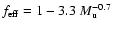
shocks. The driving efficiency
increases by about a factor
of four between runs R5_0.2.4 and R87_0.2.4. Also noteworthy is that the
absolute value of the driving power
differs by
more than 4 orders of magnitude between runs R5_0.2.4 and R87_0.2.4. The
best fit for the assumed Mach-number dependence (minimization of
.
The corresponding integral in
Eq. (24) is evaluated numerically, and the resulting driving
efficiency is shown in the top panel of Fig. 7. As
can be seen, larger Mach-numbers lead to more efficient driving, and a smaller
part of the upstream kinetic energy is thermalized already at the confining
shocks. The driving efficiency
increases by about a factor
of four between runs R5_0.2.4 and R87_0.2.4. Also noteworthy is that the
absolute value of the driving power
differs by
more than 4 orders of magnitude between runs R5_0.2.4 and R87_0.2.4. The
best fit for the assumed Mach-number dependence (minimization of
 in Eq. (25)) yields
 .
The corresponding values of
are shown in the bottom panel of
Fig. 7. From the figure we take that the second
part of our assumption a), the simple Mach-number dependence of
,
seems justified. The figure also shows that
,
and thus the driving power
,
is not strictly independent of
but decreases with
increasing .
Repeating the best fit analysis but allowing for a
linear dependence of
on
again leads to
,
while
changes from 3.1 to 3.6
as
goes from 10 to 70. The average value of
is 3.3. Omission of the extreme runs R5_0.2.4 and R87_0.2.4 does not change the
result.
.
The corresponding values of
are shown in the bottom panel of
Fig. 7. From the figure we take that the second
part of our assumption a), the simple Mach-number dependence of
,
seems justified. The figure also shows that
,
and thus the driving power
,
is not strictly independent of
but decreases with
increasing .
Repeating the best fit analysis but allowing for a
linear dependence of
on
again leads to
,
while
changes from 3.1 to 3.6
as
goes from 10 to 70. The average value of
is 3.3. Omission of the extreme runs R5_0.2.4 and R87_0.2.4 does not change the
result.
We determine the dissipated energy as
(Sect. 3.2.2), where
is the
change per time of the kinetic energy within an average column of the CDL, and
is directly from our simulation data.
Figure 8 shows the numerically obtained value
(top panel) and the theoretically expected
value (Eq. (34))
 (middle panel), both in units of
,
as well as the ratio of the two (bottom
panel). For better display, the theoretical value, which must not depend on
,
is shown as a (constant) function of
.
For the
constants in Eq. (34) we used the numerically obtained average
values,
(middle panel), both in units of
,
as well as the ratio of the two (bottom
panel). For better display, the theoretical value, which must not depend on
,
is shown as a (constant) function of
.
For the
constants in Eq. (34) we used the numerically obtained average
values,
 ,
,
and
.
We used
,
,
and
.
We used
 only for
R5_0.2.4, in accordance with the bottom panel of
Fig. 7. The numerically obtained value was
smoothed for better display using a running mean with window size
only for
R5_0.2.4, in accordance with the bottom panel of
Fig. 7. The numerically obtained value was
smoothed for better display using a running mean with window size
 .
The effect of the smoothing is illustrated in
Fig. 9 with the example of run R11_0.2.4.
.
The effect of the smoothing is illustrated in
Fig. 9 with the example of run R11_0.2.4.
![\begin{figure}
\par\includegraphics[width=8cm,clip]{3898f8a.ps}\par\vspace*{2mm}...
...b.ps}\par\vspace*{2mm}
\includegraphics[width=8cm,clip]{3898f8c.ps}
\end{figure}](/articles/aa/full/2006/43/aa3898-05/Timg279.gif) |
Figure 8:
Numerically obtained ( top panel) and theoretically expected
( middle panel) energy dissipation in units of the upstream kinetic energy
flux density
.
The constants in Eq. (34) were set to the
best fit values,
,
,
and
.
We used
for run
R5_0.2.4 (for details see text). The bottom panel shows the ratio of the
two quantities. Individual curves denote the same runs as in
Fig. 4. For better display,
was smoothed using a running mean with time window
. |
| Open with DEXTER |
![\begin{figure}
\par\includegraphics[width=8cm,clip]{3898f9.ps}
\end{figure}](/articles/aa/full/2006/43/aa3898-05/Timg280.gif) |
Figure 9:
Effect of smoothing
with a running mean and
window
,
illustrated by run R33_0.2.4. Shown is
in units of
,
before (dashed, black) and after (solid, red)
smoothing, in units of erg cm-3 s-1. |
| Open with DEXTER |
Looking at the data of
and
,
three points may be stressed. First,
(Fig. 8, top panel)
mirrors
 (Fig. 7, top panel), and the values
usually differ by less than 10%. This is not surprising. It
implies, however, that for larger upstream Mach-numbers, a larger
fraction of the upstream kinetic energy is thermalized only within the
volume of CDL and not already at its confining shocks. For
(Fig. 7, top panel), and the values
usually differ by less than 10%. This is not surprising. It
implies, however, that for larger upstream Mach-numbers, a larger
fraction of the upstream kinetic energy is thermalized only within the
volume of CDL and not already at its confining shocks. For
 ,
the energy dissipated within the CDL
exceeds 50% of the upstream kinetic energy
(Fig. 8, top panel).
,
the energy dissipated within the CDL
exceeds 50% of the upstream kinetic energy
(Fig. 8, top panel).
Second, the bottom panel of Fig. 8 shows that
and
agree to within 10% most of the time. Given
the wide range covered (5 orders of magnitude in
,
a factor of 20 in
,
and an
increase by a factor of 7 in
), we conclude that the
self-similar solution gives a good estimate.
Third, from the same figure it can be seen that
generally decreases, except for run R5_0.2.4.
Excluding R5_0.2.4, a linear fit to
 yields a decrease of 10%
as
increases from 10 to 70. A similar fit to
yields a decrease of 10%
as
increases from 10 to 70. A similar fit to
 with
with
 yields an even
slightly larger decrease of 13%. The net dissipation,
yields an even
slightly larger decrease of 13%. The net dissipation,
 ,
in fact increases
by 3%. Thus, as the CDL size increases, the absolute dissipation
within an average column decreases while the net dissipation
increases.
,
in fact increases
by 3%. Thus, as the CDL size increases, the absolute dissipation
within an average column decreases while the net dissipation
increases.
In summary, the predicted scaling laws, Eqs. (32)
to (34), are - within the range of applicability - essentially
confirmed by the simulations. The fraction of upstream kinetic energy
dissipated only within the CDL, and not at the confining shocks, thus
increases with
.
Best-fit analysis for the numerical
constants yields
 .
Both
and
decrease
slightly with increasing
.
The net dissipation rate
increases, but
only slightly (3% increase as
goes from 10 to 70).
.
Both
and
decrease
slightly with increasing
.
The net dissipation rate
increases, but
only slightly (3% increase as
goes from 10 to 70).
4.2.4 Length scales of the turbulence
In Sect. 4.2.2 we looked at the scaling properties of
the confining shocks and pointed out that shorter auto-correlation
lengths
imply smaller-scale wiggling, thus
smaller scale changes of the kinetic energy entering the CDL. In the
following, we show that the interface based quantity
is proportional to the length scale derived
from the volume properties of the turbulence. We take this as
evidence of the tight coupling between volume and interface
properties, between the turbulence and its driving.
On dimensional grounds, we can define two length scales based on
volume properties of the turbulence,
where
 is the average column integrated kinetic energy
density. Here V is again the 2D volume of the CDL, introduced
in Sect. 2.3.1. The two scales are equal up to
a numerical constant if the density and velocity are uncorrelated,
in which case we can replace the average over the product
by the product of the averages of
and v2,
is the average column integrated kinetic energy
density. Here V is again the 2D volume of the CDL, introduced
in Sect. 2.3.1. The two scales are equal up to
a numerical constant if the density and velocity are uncorrelated,
in which case we can replace the average over the product
by the product of the averages of
and v2,
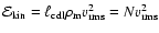 .
As this is the case in most of our simulations we look at only one of
the above quantities in the following,
.
As this is the case in most of our simulations we look at only one of
the above quantities in the following,
 ,
shown in
the top panel of Fig. 10. For better display, as
inherits the large time variability
of
,
it is smoothed in the same way as
in the bottom panel of
Fig. 8.
,
shown in
the top panel of Fig. 10. For better display, as
inherits the large time variability
of
,
it is smoothed in the same way as
in the bottom panel of
Fig. 8.
![\begin{figure}
\par\includegraphics[width=8cm,clip]{3898f10a.ps}\par\vspace*{2mm...
...b.ps}\par\vspace*{2mm}
\includegraphics[width=8cm,clip]{3898f10c.ps}\end{figure}](/articles/aa/full/2006/43/aa3898-05/Timg295.gif) |
Figure 10:
Characteristic length
of
the turbulence ( top), in units of
( middle),
and scaled with best-fit
 ( bottom) as functions of .
Individual curves denote the
same runs as in Fig. 4. For better display,
( bottom) as functions of .
Individual curves denote the
same runs as in Fig. 4. For better display,
 was smoothed by a running mean with window
.
was smoothed by a running mean with window
. |
| Open with DEXTER |
![\begin{figure}
\par\includegraphics[width=7.8cm,clip]{3898f11a.ps}\par\vspace{2mm}
\includegraphics[width=7.8cm,clip]{3898f11b.ps}
\end{figure}](/articles/aa/full/2006/43/aa3898-05/Timg298.gif) |
Figure 11:
Plots of
 for two runs that are
identical except for their upstream Mach-number. Larger upstream
Mach-numbers lead, on average, to finer structure within the CDL and
smaller scale wiggling of the confining shocks. Shown are runs
R33_0.2.4 ( top) and R11_0.2.4 ( bottom), both at a time when
for two runs that are
identical except for their upstream Mach-number. Larger upstream
Mach-numbers lead, on average, to finer structure within the CDL and
smaller scale wiggling of the confining shocks. Shown are runs
R33_0.2.4 ( top) and R11_0.2.4 ( bottom), both at a time when
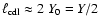 .
Blue (dark lines) indicates convergence, red (dark
patches) divergence. .
Blue (dark lines) indicates convergence, red (dark
patches) divergence. |
| Open with DEXTER |
Assuming a relation of the form
 ,
we obtain optimal
fits (minimum of
,
we obtain optimal
fits (minimum of
 )
for
)
for
 .
The fits become only
slightly better if a weak linear dependence of
.
The fits become only
slightly better if a weak linear dependence of
 on
is allowed (13% change as
goes from 10 to 70).
on
is allowed (13% change as
goes from 10 to 70).
 is shown in the middle panel of
Fig. 10. Looking directly at the dependence of
on
and
,
we find
is shown in the middle panel of
Fig. 10. Looking directly at the dependence of
on
and
,
we find
 .
This is the same dependence we
found for
in Sect. 4.2.2,
scaled with this best fit is shown in the
bottom panel of Fig. 10.
.
This is the same dependence we
found for
in Sect. 4.2.2,
scaled with this best fit is shown in the
bottom panel of Fig. 10.
With increasing upstream Mach-number the characteristic length scale
thus decreases with respect to the CDL
extension. This is consistent with our observation that for the same
the interior of the CDL shows finer structuring
(patches, filaments) for higher values of
.
Figure 11 illustrates this observation with the
example of runs R11_0.2.4 and R33_0.2.4. Shown in the figure is
,
as the flow patterns, especially shocks, are
better visible in this quantity than in density.
In summary, our simulations show that the inherent length scale of the
turbulence is proportional to the auto-correlation length of the
confining shocks, independent of
and
.
With increasing
,
both length
scales decrease relative to the CDL extension,
 .
The appearance of the CDL, the size of its
patches and filaments, behaves similarly.
.
The appearance of the CDL, the size of its
patches and filaments, behaves similarly.
4.3 Settings with CDL at t = 0
![\begin{figure}
\par\hspace*{2mm}\includegraphics[width=8cm,clip]{3898f12a.ps}\pa...
...s}\par\vspace*{2mm}
\includegraphics[width=8.2cm,clip]{3898f12d.ps}
\end{figure}](/articles/aa/full/2006/43/aa3898-05/Timg306.gif) |
Figure 12:
Comparing runs with and without an initial CDL. Shown are
(first),
(second), the scaled driving
efficiency
 (third), and
the scaled characteristic length of the turbulence
(third), and
the scaled characteristic length of the turbulence
 for all symmetric runs. Line styles and colors
denote initial conditions, 0 (solid line, blue), 1 (dashed line, red),
and 2 (dash-dotted line, orange).
for all symmetric runs. Line styles and colors
denote initial conditions, 0 (solid line, blue), 1 (dashed line, red),
and 2 (dash-dotted line, orange). |
| Open with DEXTER |
![\begin{figure}
\par\includegraphics[width=8.8cm,clip]{3898f13.ps}
\end{figure}](/articles/aa/full/2006/43/aa3898-05/Timg307.gif) |
Figure 13:
Time evolution of angle distribution for run R22_2.2.2.
Shown is the average angle distribution for
 (dashed, blue),
 (dash-dotted, green),
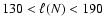 (dash-three-dots, orange),
 (long dashes, purple),
 (solid, red).
Also shown are the distributions for run R5_0.2.4 (black dots, right line) and
for run R11_0.2.4 (black dots, left line), both averaged
over
.
(solid, red).
Also shown are the distributions for run R5_0.2.4 (black dots, right line) and
for run R11_0.2.4 (black dots, left line), both averaged
over
. |
| Open with DEXTER |
We performed additional runs to study the influence of an initially
present CDL. Figure 12 illustrates the results for
some selected quantities. Shown are all the runs we
performed with initial condition I=0 (no CDL at
t=0), I=1 (moderate CDL at t=0), and I=2 (massive CDL at t=0).
Comparison of the I=1 and I=0 curves in Fig. 12 shows that an
initially present CDL of moderate column density (
)
soon develops characteristics similar to those found in simulations without
initial CDL. A quasi-steady state is reached for
 .
The
I=1 and I=0 curves then agree to within about a factor of two for volume
quantities like
and
(first two panels
in Fig. 12). Agreement seems slightly better for interface
related quantities. For
.
The
I=1 and I=0 curves then agree to within about a factor of two for volume
quantities like
and
(first two panels
in Fig. 12). Agreement seems slightly better for interface
related quantities. For
 ,
shown in the third
panel of Fig. 12, the I=1 and I=0 curves lie more or less on
top of each other. The same is true for
,
shown in the third
panel of Fig. 12, the I=1 and I=0 curves lie more or less on
top of each other. The same is true for
 ,
shown in the bottom panel of
Fig. 12.
,
shown in the bottom panel of
Fig. 12.
The situation is slightly different for runs with an initially rather massive
CDL (I=2, with initially
). Also in these simulations
the CDL gets more and more turbulent. For all the quantities shown in
Fig. 12, the I=2 curves approach the I=1 and I=0 curves.
However, it takes these runs much longer to saturate. Only for
 the curves finally seem to saturate, at similar values as the I=0 and I=1curves. That saturation does indeed occur around that time is also supported
by Fig. 13. As can be seen, the average angle
distribution of the confining shocks for run R22_2.2.2 first shifts to higher
and higher values as
increases. It then stagnates for the last
two averaging periods,
and
.
the curves finally seem to saturate, at similar values as the I=0 and I=1curves. That saturation does indeed occur around that time is also supported
by Fig. 13. As can be seen, the average angle
distribution of the confining shocks for run R22_2.2.2 first shifts to higher
and higher values as
increases. It then stagnates for the last
two averaging periods,
and
.
In summary, we conclude that our symmetric simulations all end up in a
similar quasi-steady final state. An initially present CDL only delays
the development. The incoming flows also manage to generate (and sustain) a
similar level of turbulence also within an initially massive CDL.
![\begin{figure}
\par\includegraphics[width=8.8cm,clip]{3898f14.ps}\end{figure}](/articles/aa/full/2006/43/aa3898-05/Timg313.gif) |
Figure 14:
Average
as a function of
for
all our symmetric simulations (triangles). In addition, we included
data from our asymmetric runs (asterisks), for which
 and which initially have no CDL.
Averages were taken over
for simulations
without initial CDL (blue triangles and green asterisks), over
and which initially have no CDL.
Averages were taken over
for simulations
without initial CDL (blue triangles and green asterisks), over
 for runs with a moderate initial CDL
(red triangles), and over
for runs with a moderate initial CDL
(red triangles), and over
 for runs with a
massive initial CDL (orange triangles). Lines show
for runs with a
massive initial CDL (orange triangles). Lines show
 with
with  (dashed) and
 (dotted).
 |
| Open with DEXTER |
4.4 Asymmetric cases
We also computed a few asymmetric cases, where the two upwind Mach-numbers are
different,
 .
For the same reason as given
in Sect. 3, we expect the solution to only depend on
.
For the same reason as given
in Sect. 3, we expect the solution to only depend on
 and
and
 .
These dependencies are more
complicated than those assumed in Sect. 3 as we now have
two different upwind Mach-numbers. The simple dependencies of
Sect. 3 should, however, be recovered in the limit
.
These dependencies are more
complicated than those assumed in Sect. 3 as we now have
two different upwind Mach-numbers. The simple dependencies of
Sect. 3 should, however, be recovered in the limit
 .
.
The basic physical reason for the more complicated dependencies on the
upwind Mach-numbers lies in the strong back coupling between the
turbulence within the CDL and the driving of this turbulence by the
upwind flows. Our asymmetric simulations demonstrate clearly (much
more clearly than the symmetric simulations) that the turbulence
crucially affects the driving: although
and
are strongly different, the corresponding driving
efficiencies are about equal,
 .
Thus the efficiency does not depend primarily on
the upwind flow. In fact, Fig. 14 shows that for
both symmetric and asymmetric runs
(averaged now
over both shocks) can be described well by
.
Thus the efficiency does not depend primarily on
the upwind flow. In fact, Fig. 14 shows that for
both symmetric and asymmetric runs
(averaged now
over both shocks) can be described well by
 |
(43) |
The angle distribution of the two shocks behaves accordingly in that
it is similar for both shocks and determined by
rather than by either
or
.
A more detailed analysis of the asymmetric case, including an
approximate analytical solution, will be presented in a
subsequent paper.
4.5 Grid and domain studies
The numerical results presented in Sect. 4.2
were all based on simulations with a domain
 and a discretization of
(R=2) or 2560 cells in the y-direction. Here we
want to check whether these choices have any systematical effect on
the numerical results of Sect. 4.2.
and a discretization of
(R=2) or 2560 cells in the y-direction. Here we
want to check whether these choices have any systematical effect on
the numerical results of Sect. 4.2.
4.5.1 Different y-extent
To check whether the size of the computational domain has any
systematic effect on the results of Sect. 4.2,
we performed some of the simulations again, but this time on smaller
domains of
 and
and
 .
We also performed one simulation
on a larger domain
.
We also performed one simulation
on a larger domain
 .
.
Figure 15 illustrates our findings for
simulations on domains
and
.
shows no
systematic effect and is, as such, representative of other volume-related
quantities (Fig. 15, top panel). As a typical
representative for interface-related quantities,
also shows
no clear overall effect of the domain size
(Fig. 15, middle panel). The quantity for which
we find the most clear effect is the auto-correlation length
(Fig. 15, bottom panel).
However, even for
the effect sets in only for two of
the four runs and only for
 ,
i.e. once the CDL
extension reaches about half the size of the smaller domain. For the
numerical results in Sect. 4.2,
corresponds to
.
We conclude that the
y-extent of the computational domain has no apparent systematic effect on
these results up to
,
i.e. once the CDL
extension reaches about half the size of the smaller domain. For the
numerical results in Sect. 4.2,
corresponds to
.
We conclude that the
y-extent of the computational domain has no apparent systematic effect on
these results up to
 and probably even up to
 .
.
A systematic effect of the computational domain on the numerical solution does
become apparent if the simulations are carried on much longer. One pair of
runs, R22_0.2.2 and R22_0.2.6, were carried on much longer, till
 .
For this pair of runs, Fig. 16 shows the
evolution of
for each run, as well as their ratio,
.
For this pair of runs, Fig. 16 shows the
evolution of
for each run, as well as their ratio,
 .
The run on the smaller domain
apparently shows a faster decay in
after
.
The run on the smaller domain
apparently shows a faster decay in
after
 .
From Fig. 17 we take that the behavior
of this one pair of runs is most likely the rule, and not the exception. The
top panel of Fig. 17 shows
,
scaled, for all the symmetric runs we have performed and whose domain has a
y-extent
.
From Fig. 17 we take that the behavior
of this one pair of runs is most likely the rule, and not the exception. The
top panel of Fig. 17 shows
,
scaled, for all the symmetric runs we have performed and whose domain has a
y-extent 
 .
The bottom panel of
Fig. 17 gives the same quantity for all the runs with a
domain extention
.
The bottom panel of
Fig. 17 gives the same quantity for all the runs with a
domain extention 
 .
Comparison of the two
figures shows that runs on a domain
saturate
around
.
Comparison of the two
figures shows that runs on a domain
saturate
around
 .
For runs on a domain
,
reaches much higher values.
.
For runs on a domain
,
reaches much higher values.
![\begin{figure}
\par\includegraphics[width=8.1cm,clip]{3898f15a.ps}\par\vspace*{2...
....ps}\par\vspace*{2mm}
\includegraphics[width=8cm,clip]{3898f15c.ps}
\end{figure}](/articles/aa/full/2006/43/aa3898-05/Timg337.gif) |
Figure 15:
Comparing runs that differ only in the y-extent of the
domain (
 and
and
 ). Shown are ). Shown are
 ( top),
 ( middle), and
 ( bottom). Individual curves denote
runs R11_0.2.* (dashed, purple), R22_0.2.* (solid, red),
R33_0.2.* (dash-dotted, orange), R43_0.2.* (dash-three-dots,
green).
( bottom). Individual curves denote
runs R11_0.2.* (dashed, purple), R22_0.2.* (solid, red),
R33_0.2.* (dash-dotted, orange), R43_0.2.* (dash-three-dots,
green). |
| Open with DEXTER |
![\begin{figure}
\par\includegraphics[width=8.2cm,clip]{3898f16a.ps}\par\vspace*{2mm}
\hspace*{1mm}\includegraphics[width=8.2cm,clip]{3898f16b.ps}\end{figure}](/articles/aa/full/2006/43/aa3898-05/Timg338.gif) |
Figure 16:
Comparison of runs R22_0.2.2 and R22_0.2.6, illustrating
the effect of a three-times larger y-extent of the computational
domain on long time scales. Shown are
( top) for R22_0.2.2 (solid,
light blue) and R22_0.2.6 (dashed, dark red) and the ratio
 ( bottom).
 |
| Open with DEXTER |
![\begin{figure}
\par\includegraphics[width=8cm,clip]{3898f17a.ps}\par\vspace*{2mm}
\includegraphics[width=8.1cm,clip]{3898f17b.ps}
\end{figure}](/articles/aa/full/2006/43/aa3898-05/Timg340.gif) |
Figure 17:
Scaled auto-correlation lengths
of all symmetric simulations on domains with a y-extent less or equal
to
 ( top) and a y-extent greater or
equal to
( bottom).
( top) and a y-extent greater or
equal to
( bottom). |
| Open with DEXTER |
4.5.2 Different discretization
The results presented in Sect. 4.2 were all based on
simulations with a discretization of
(R=2) or 2560 cells in the y-direction. To check the
effect of the discretization on our results, we repeated several
simulations with coarser and/or finer discretization. These simulations
indeed reveal a systematic effect of the discretization on the values of
average quantities. Nevertheless, the general properties of the solution, its
approximate self-similarity and Mach-number dependences, remain unaltered.
Only the numerical constants
are affected. The changes
are, however, small when compared to the differences between the 1D and 2D
solution (for example,
 in 2D, while
 in 1D).
We find that finer discretization generally leads to reduced turbulence.
Using finer meshes we obtained larger mean densities and lower values of
,
as shown in Fig. 18. The driving
efficiency gets lower and the shocks become more inclined with respect to the
direction of the upstream flows, and the angle distribution is shifted to
lower values. The characteristic length scale
remains about constant if taken in units of
.
A possible explanation for the reduction of turbulence (smaller
)
on finer grids could be the dominance of shocks
for the energy dissipation in the CDL. On a coarser grid, the network
of shocks within the CDL is less dense. The divergence plots shown in
Fig. 19 illustrate this effect. A closer
analysis of this idea is, however, beyond the scope of the present
paper.
![\begin{figure}
\par\includegraphics[width=8.8cm,clip]{3898f18.ps}
\end{figure}](/articles/aa/full/2006/43/aa3898-05/Timg343.gif) |
Figure 18:
Comparison of
for runs whose spatial resolution
differs by a factor of 2 (subscript c = coarse, f = fine). Shown
are (giving only the name of the finer run) runs R22_0.2.4 (solid,
red), R22_0.4.4 (dash-three-dots, blue), R43_0.2.4 (long dashes,
purple), and R11_0.2.4 (dash-dotted, orange). |
| Open with DEXTER |
![\begin{figure}
\par\includegraphics[width=8cm,clip]{3898f19a.ps}\par\vspace{2mm}
\includegraphics[width=8cm,clip]{3898f19b.ps}
\end{figure}](/articles/aa/full/2006/43/aa3898-05/Timg344.gif) |
Figure 19:
Plots of
for two runs that are identical
to run R11_0.2.4, shown in Fig. 11, except for
their discretization. The runs shown here were computed with two times lower
( top) and at four times lower ( bottom) resolution. Blue (dark lines)
indicates convergence, red (dark patches) divergence. As can be seen, the
number of convergent regions within an average CDL column decreases with
decreasing resolution. |
| Open with DEXTER |
We stress that, so far, no convergence has been reached in our discretization
studies. Looking at the comparison of the three runs R22_0.1.4,
R22_0.2.4, and R22_0.4.4 in Fig.18 shows that each
reduction of the cell size by a factor of two leads to a reduction of
about 20% in
.
This indicates that the resolution
of 2560 cells in y-direction in our standard runs (R*_0.2.4) and of
5120 cells in the y-direction in the refined runs is still not
sufficient. This should be kept in mind when interpreting these
results or any results on shock bound turbulent structures
in 2D, let alone 3D.
Also, no clear picture emerges regarding the deviation of
from the constant value predicted by Eq. (15). A linear fit to
for
yields -12% for run
R22_0.2.4 and -23% for the two times coarser run R22_0.1.4. For runs
R43_0.*.4, the grid dependence is the other way round: R43_0.2.4 shows a
decrease of -25%, the twice coarser run R43_0.1.4 decreases by only -15%.
5 Discussion
We want to address four points in this section. First, we sketch
possible reasons for the slight difference between the numerical
solution and the relations we derived in Sect. 3.
Second, we look once more at the driving of the turbulence and, in
particular, the back-coupling between interface and volume properties.
Third, we briefly consider our results in an astrophysical context, in
particular with regard to molecular clouds. Finally, based on
preliminary numerical results, we sketch the effect of some additional
physics.
In Sect. 3.2 we suggested that a self-similar
solution to our 2D model problem may still exist for the limiting case
where the system approaches infinity. The relations derived in that
section give a reasonable estimate for the numerical results of
Sect. 4. However, while
is
constant in Sect. 3.2, the numerical simulations
show a gradual decrease in
already for small CDLs,
 (15% decrease of
as
increases from 10 to 70,
Sect. 4.2). We have no firm explanation for this
difference. We sketch three possible effects in the following, but
stress that the available data do not allow us to clearly distinguish
between them.
(15% decrease of
as
increases from 10 to 70,
Sect. 4.2). We have no firm explanation for this
difference. We sketch three possible effects in the following, but
stress that the available data do not allow us to clearly distinguish
between them.
A first, obvious reason could be the finite y-extent of the computational
domain, Y. It sets an upper limit on the total energy input into
the CDL, thus on the amount of mass within the CDL that can be driven. Once
the CDL has accumulated too much mass, the driving per unit mass weakens and
the turbulence starts to weaken. The spatial growth of the CDL slows down
while the average density increases. The following considerations on time
scales may illustrate this point further.
An upper limit to the time at which Y starts to affect the solution
is given by the time ty at which
 .
At later times structures may still grow in the x-direction (up
to
at most) but cannot grow any more in the y-direction
(where Y sets an upper limit). For the runs in
Sect. 4.2,
corresponds to
.
At later times structures may still grow in the x-direction (up
to
at most) but cannot grow any more in the y-direction
(where Y sets an upper limit). For the runs in
Sect. 4.2,
corresponds to
 or
or
 .
A lower limit for the decay time
scale of the turbulence may be obtained as follows. For the case of uniformly
driven isothermal hydrodynamic turbulence in a 3D periodic box,
Mac Low (1999) has shown that the typical decay time once the driving is
turned off,
.
A lower limit for the decay time
scale of the turbulence may be obtained as follows. For the case of uniformly
driven isothermal hydrodynamic turbulence in a 3D periodic box,
Mac Low (1999) has shown that the typical decay time once the driving is
turned off,
 ,
and the initial driving wave length,
,
and the initial driving wave length,
 ,
are related by
,
are related by
 .
Assuming that this result also
holds for our slab, that
.
Assuming that this result also
holds for our slab, that
 ,
and that
driving is turned off completely, it follows that
,
and that
driving is turned off completely, it follows that
 ,
or
,
or
 for the runs in
Sect. 4.2. However, driving continues in our simulations
and so the effective decay time scale of the turbulence is likely to be much
longer than
.
Finally, for the runs in
Sect. 4.2, and a typical integration time of
corresponds to about
for the runs in
Sect. 4.2. However, driving continues in our simulations
and so the effective decay time scale of the turbulence is likely to be much
longer than
.
Finally, for the runs in
Sect. 4.2, and a typical integration time of
corresponds to about
 ,
a typical turbulent crossing time at
)
is
,
a typical turbulent crossing time at
)
is
 .
Comparing these different time
scales makes it seem likely that at
,
turbulence in the center
of the CDL is still essentially driven, not essentially decaying.
.
Comparing these different time
scales makes it seem likely that at
,
turbulence in the center
of the CDL is still essentially driven, not essentially decaying.
Our simulation data do not allow us to either clearly confirm or reject the
hypothesis that the finite y-extent of the computational domain is responsible
for the slight decrease in
that we observe at early times,
 .
If the finite domain size were responsible,
should decay differently on different domains. Comparison
of simulations on different domains up to
.
If the finite domain size were responsible,
should decay differently on different domains. Comparison
of simulations on different domains up to
 (Sect. 4.5.1), however, gives no clear picture. The data are
rather noisy, and simulations on domains
and
show no systematic differences as long as
(
(Sect. 4.5.1), however, gives no clear picture. The data are
rather noisy, and simulations on domains
and
show no systematic differences as long as
(
 on the smaller domain).
Only for much later times,
on the smaller domain).
Only for much later times,
 ,
well beyond the range for the
results in Sect. 4.2, does Y have a clear
effect and
decreases faster on smaller domains
(Fig. 16).
,
well beyond the range for the
results in Sect. 4.2, does Y have a clear
effect and
decreases faster on smaller domains
(Fig. 16).
A second, more speculative, reason might be numerical dissipation,
provided that its effect were to increase with
.
While we have no evidence that the latter is really the case, it may
also be hasty to discard this possibility right away.
Porter & Woodward (1994) found, by observing how simple 2D
hydrodynamical flows (shear flows and sound waves of definite wave
number, their Sect. 3.3) damp with time, that the decay rate due to
numerical dissipation alone is a non-linear function of the wave
number. Their results are certainly not directly applicable to the
present case. But in view of these results, and given the change in
structure size with
as suggested by
Fig. 3, it might be possible that the effect of
numerical dissipation indeed changes with
.
Note
that this would also imply that the MILES approach, outlined in
Sect. 2.1, were not strictly valid for the problem we
consider. The currently available data do not allow us to clearly
reject or confirm the effect.
A third reason, or rather an amplifying mechanism, could be back-coupling
between
and the driving efficiency. Once the turbulence
within the CDL is slightly reduced (for whatever reason), the reduction is
further amplified by the back-coupling between turbulence and driving,
 .
The decrease in
results in larger inclination of the shocks with respect to
the direction of the upstream flows, more energy is dissipated at the
confining shocks of the CDL, and less driving energy enters the CDL. For the
observed 15% reduction of
,
the reduced driving may, in
fact, play a dominant role: as
increases from 10 to 70,
decreases by 13% (Sect. 4.2.3). But to really estimate
the relative importance of the three effects just sketched, further studies
are certainly necessary.
.
The decrease in
results in larger inclination of the shocks with respect to
the direction of the upstream flows, more energy is dissipated at the
confining shocks of the CDL, and less driving energy enters the CDL. For the
observed 15% reduction of
,
the reduced driving may, in
fact, play a dominant role: as
increases from 10 to 70,
decreases by 13% (Sect. 4.2.3). But to really estimate
the relative importance of the three effects just sketched, further studies
are certainly necessary.
Two more points seem noteworthy to us in this section. One concerns the near
independence of
on
.
From
Fig. 3 (increase in structure size with increasing
), we take that it is rather the increasing average
distance between shocks that allows
to be
essentially independent of
and not so much the, on
average, decreasing strength of shocks (Sect. 3.2.3).
Whether this is indeed true, only a closer analysis of the structure within
the CDL along the lines of Mac Low & Ossenkopf (2000) can tell, which is,
however, beyond the scope of the present paper. Such an analysis could also
shed light on whether (or in which sense)
(see Sect. 4.2.3) is indeed a measure of the average
distance between shocks. It would also allow us to quantify our impression that
small scale structures are preferably located close to the confining
interfaces. If true, this would fit with the result by Smith et al. (2000)
that the high-frequency part of the shock spectrum is lost most efficiently.
The other point concerns run R5_0.2.4. With corr
,
it violates two of the basic
assumptions we made in Sect. 3.2. Its mean
density is close to the isothermal value for strong shocks,
 .
Both
and
increase with
.
With these characteristics, R5_0.2.4 may mark
the transition from compressible supersonic turbulence, the topic of
this paper, to compressible subsonic turbulence.
.
Both
and
increase with
.
With these characteristics, R5_0.2.4 may mark
the transition from compressible supersonic turbulence, the topic of
this paper, to compressible subsonic turbulence.
The turbulence within the CDL is "naturally driven'' in the sense that
we control neither what fraction of the total upstream kinetic energy,
 ,
really enters the CDL nor the
spatial scale on which this energy input varies. Both are directly
determined by the confining shocks instead and indirectly depend on
the system as a whole. The driving efficiency at each confining shock
scales with
,
even for situations where
(see
Sect. 4.4). The auto-correlation length of the
confining shocks and the characteristic length scale of the turbulence
within the CDL are proportional to each other, both scaling as
,
really enters the CDL nor the
spatial scale on which this energy input varies. Both are directly
determined by the confining shocks instead and indirectly depend on
the system as a whole. The driving efficiency at each confining shock
scales with
,
even for situations where
(see
Sect. 4.4). The auto-correlation length of the
confining shocks and the characteristic length scale of the turbulence
within the CDL are proportional to each other, both scaling as
 .
We take these facts as
evidence that the CDL as a whole, its interface and volume properties,
forms a tightly coupled, quasi-stationary, and self-regulating system.
Back coupling between post shock flow and shock is also described in
other contexts, for example by Foglizzo (2002) for the case of
Bondi-Hoyle accretion.
.
We take these facts as
evidence that the CDL as a whole, its interface and volume properties,
forms a tightly coupled, quasi-stationary, and self-regulating system.
Back coupling between post shock flow and shock is also described in
other contexts, for example by Foglizzo (2002) for the case of
Bondi-Hoyle accretion.
An aspect that remained elusive in Sect. 4 is the
spatial scale on which the energy input varies, the energy injection
scale. To really tackle this issue, it would be necessary to analyze
the energy spectrum of the CDL. This task requires, however, some
caution because of the highly irregular boundary of the CDL, and we
postpone it for the moment. Nevertheless, we would like to present a
few thoughts on the subject.
A first question is whether it is justified to speak at all of only
one injection scale, of monochromatic driving. The homogeneous
upstream flow is modulated by the confining shocks. These are wiggled
on a variety of spatial scales at any given moment. This strongly
suggests that the kinetic energy input into the CDL is most likely not
monochromatic but occurs at a whole spectral range instead.
Consequences of such non-monochromatic driving have been studied, for
example, by Norman & Ferrara (1996).
It also seems worthwhile to briefly look at monochromatically-driven
turbulence, in particular at the numerical simulations by Mac Low (1999).
For the case of artificially, monochromatically driven hydrodynamic turbulence
in a 3D box with periodic boundaries, he found that the characteristic length
of the turbulence is proportional to the driving wave length, independent of
the Mach-number:
 ,
where
,
where  is the (known) driving wave length and
 is the 3D analogon of
in Eq. (41). In addition,
Mac Low (1999) observed that
increases with ,
which is mirrored in the apparent increase in the structure size (patches,
filaments).
is the 3D analogon of
in Eq. (41). In addition,
Mac Low (1999) observed that
increases with ,
which is mirrored in the apparent increase in the structure size (patches,
filaments).
Although our setting clearly differs from that of Mac Low (1999),
two thoughts come to mind. The first is an actual observation,
namely that we also observe an increase in structure size with
.
The second thought is more of a
question or speculation. Mac Low (1999) determines the
proportionality constant between the characteristic scale of the
turbulence and the monochromatic driving wave length. One may wonder
about the implications of this finding if not one driving wave length
is present but a whole spectrum. How will the characteristic length
scale of the turbulence, which can still be determined following
Eq. (41), depend on this spectrum? And, given our
finding that
 ,
what does
tell us about
this spectrum? Both questions should become tractable once the energy
spectrum of the CDL is determined.
,
what does
tell us about
this spectrum? Both questions should become tractable once the energy
spectrum of the CDL is determined.
With regard to astrophysics, the presented work basically suggests
that, within the frame of isothermal hydrodynamics and a roughly plane
parallel setting, larger Mach-numbers of the colliding flows results
in a finer and finer network of higher and higher density contrast
within the interaction zone. In different types of wind-driven
structures, this connection between Mach-number and structure may be
directly observable.
For the clumping of line-driven hot-star winds, our results suggest
that the sheets or clumps formed by the instability of the
line-driving are not homogeneous but possess fine-scale substructure
with high density contrast.
Concerning molecular clouds, we first mention that recent arguments
support the idea, originally brought forward by Hunter (1979) and
Larson (1981), that molecular clouds result from the collision of
large-scale flows in the ISM. Basu & Murali (2001) make the point
that small-scale driving ( 0.1-1 pc) of molecular clouds is
incompatible with observed total luminosities, unless the energy
dissipation rates derived from MHD simulations are seriously
overestimated. Using a principal component analysis of
0.1-1 pc) of molecular clouds is
incompatible with observed total luminosities, unless the energy
dissipation rates derived from MHD simulations are seriously
overestimated. Using a principal component analysis of
 CO (J=1-0) emission, Brunt (2003) identifies
large-scale flows of atomic material in which the globally turbulent
molecular clouds are embedded. Similar observational results were
reported by Ballesteros-Paredes et al. (1999a).
CO (J=1-0) emission, Brunt (2003) identifies
large-scale flows of atomic material in which the globally turbulent
molecular clouds are embedded. Similar observational results were
reported by Ballesteros-Paredes et al. (1999a).
Driven supersonic turbulence as a structuring agent for the interior
of molecular clouds was examined by many authors
(Audit & Hennebelle 2005; Elmegreen 1993; Ballesteros-Paredes et al. 1999a; Mac Low 1999; Mac Low & Klessen 2004; Hartmann et al. 2001; Vazquez-Semadent et al. 1995; Burkert & Hartmann 2004; Hunter et al. 1986; Vázquez-Semadeni et al. 2006; Joung & Mac Low 2004; Heitsch et al. 2005; Ballesteros-Paredes et al. 2006; Kim & Ryu 2005; Mac Low et al. 1998; Ballesteros-Paredes et al. 1999b). The driving wave length of the
turbulence, and thus the largest structure size (Mac Low 1999; Ballesteros-Paredes & Mac Low 2002), is usually a free parameter. Our results
show instead that, at least for the case of an isothermal, shock
compressed, supersonically turbulent 2D slab, the structure size
rather depends on the size of the slab or cloud.
The model presented in this paper covers only some very basic physics. To
obtain results with a more direct relation to reality, additional physics
must be included in the future, among these the following. Strongly
asymmetric flows, where
,
lead to more
complicated dependences, as we will demonstrate in a forthcoming paper.
Inclusion of radiative cooling, instead of assuming isothermal conditions,
can affect the problem in different ways. Thermal instability can lead to
additional dynamical effects (Audit & Hennebelle 2005; Chevalier & Imamura 1982; Walder & Folini 1996; Hennebelle & Pérault 2000,1999; Mignone 2005; Koyama & Inutsuka 2002; Heitsch et al. 2005; Pittard et al. 2005; Vázquez-Semadeni et al. 2000; Strickland & Blondin 1995; Gaetz et al. 1988). Extended
cooling layers, on the other hand, tend to act as a cushion. Simulations
by Walder & Folini (1999) and Walder & Folini (2000b), which include radiative
cooling but have otherwise similar parameters as some of the simulations
presented here, show comparatively more small scale structure and even
roll-ups at the interfaces confining the CDL. The CDL as a whole evolves
less violently, and mean densities are about a factor of four to eight higher
that what we found here for the isothermal case. Strongly asymmetric flows,
where
,
lead to a qualitatively different
solution if radiative cooling is included (Walder & Folini 1998) and to
more complicated dependences on the upwind Mach-numbers in the isothermal
case, as we will demonstrate in a forthcoming paper. The role of thermal
conduction has only been considered by relatively few publications so
far (Koyama & Inutsuka 2004; Begelman & McKee 1990; Myasnikov & Zhekov 1998).
Global bending of the interaction zone affects the stability properties of the
interaction zone as a whole and thus probably also its interior properties.
In colliding wind binaries, for example, matter is transported out of the
central part of the system and diluted in the outer part. Simulations of bow
shocks and colliding winds in binaries show strong traveling waves, together
with a systematic change of the mean properties in the flow off from the
stagnation point (Stevens et al. 1992; Walder & Folini 1995; Blondin & Koerwer 1998).
6 Summary and conclusions
We looked at symmetric, supersonic (
), isothermal, plane-parallel, colliding flows in 2D. The
resulting shock-confined interaction zone (CDL) is supersonically
turbulent (
 ). We investigated
the CDL and its interplay with the upstream flows by dimensional
analysis and numerical simulations. The latter we generally stopped
when
.
The results are
interesting not only with regard to flow collisions, but also shed new
light on the properties of supersonic turbulence in general.
). We investigated
the CDL and its interplay with the upstream flows by dimensional
analysis and numerical simulations. The latter we generally stopped
when
.
The results are
interesting not only with regard to flow collisions, but also shed new
light on the properties of supersonic turbulence in general.
The numerical simulations show that the CDL has an irregular shape and a
patchy, supersonically turbulent interior. The driving of the turbulence is
natural in that it depends on the shape of the confining shocks. The
dimensional analysis is based on isothermal Euler equations in infinite space.
Within this frame, a self-similar solution may exist that would depend on
but must not depend on
.
Relations for
average quantities are obtained under some further simplifying assumptions
(Sect. 3.3).
Based on both the analytical and numerical results, we arrive at the following
conclusions.
- 1.
- Comparison of the numerical and the self-similar solution shows
generally good agreement if
 .
The modest
deviation between the numerical and the self-similar solutions
increases with
.
We suggest some explanations for
the deviation, but our data do not allow any clear conclusions on the
issue. For
.
The modest
deviation between the numerical and the self-similar solutions
increases with
.
We suggest some explanations for
the deviation, but our data do not allow any clear conclusions on the
issue. For
 ,
we have but one simulation.
It shows clear differences to the other runs and may be more
characteristic of compressible subsonic turbulence than of
supersonic turbulence;
,
we have but one simulation.
It shows clear differences to the other runs and may be more
characteristic of compressible subsonic turbulence than of
supersonic turbulence;
- 2.
- The CDL is characterized by
 and
.
The average compression
ratio of the CDL is thus independent of
.
This is in
sharp contrast to the 1D case, where
and
.
The average compression
ratio of the CDL is thus independent of
.
This is in
sharp contrast to the 1D case, where
 .
From the numerical simulations,
we find
.
From the numerical simulations,
we find
 ;
;
- 3.
- The turbulence within the CDL and the driving efficiency are related by
.
The relation also holds for
asymmetric settings, where
,
emphasizing
the mutual coupling between volume and interface properties. For larger
upstream Mach-numbers, the shocks confining the interaction zone are less
strongly inclined with respect to the direction of the upstream flows. The
driving is more efficient, a larger fraction of the upstream kinetic energy is
dissipated only within the CDL and not already at the confining shocks;
- 4.
- The characteristic length scale of the turbulence,
,
and the auto-correlation length of
the confining shocks,
,
are proportional to each
other. Both scale as
,
this
although the former is based on volume quantities while the latter is
derived from interface properties;
- 5.
- The separation of filaments and the size of patches within the CDL
both get larger as
increases and/or
decreases.
For increasing upstream Mach-numbers in summary we thus expect a faster
expanding CDL with less strongly inclined confining interfaces with respect to
the direction of the upstream flows, similar mean density, finer interior
structure relative to the CDL size, and a gradual shift of the energy
dissipation from the confining shocks to internal shocks within the CDL. We
expect to observe these general dependencies in real objects where
shock-confined slabs play a role, like molecular clouds, wind driven
structures, supernova remnants, or -ray bursts.
Acknowledgements
The authors wish to thank the crew running the Cray SV1 at ETH
Zürich, where the simulations were performed, the system
administrator of the institute for astronomy, ETH Zürich, P.
Steiner, for steady support, and J. Favre from the Swiss Center of
Scientific Computing CSCS/SCSC, Manno, for graphics support. The
authors also would like to thank the referee, E. Vazquez-Semadeni,
for the detailed and engaged report.
Appendix A: numerical computation of obliqueness angle
While shocks are smeared over approximately 3 grid cells in our
simulations, the confining shocks in our analysis are specified as a
series of discrete x,y-coordinate pairs only (see
Sect. 4.2.2). This information is sufficient to
compute most shock-related quantities to good accuracy, for example
the shock length
 .
The only quantity that requires
a more careful proceeding is the obliqueness angle .
If it
were computed directly from the discrete shock positions, only
discrete values would be obtained, for example 0
.
The only quantity that requires
a more careful proceeding is the obliqueness angle .
If it
were computed directly from the discrete shock positions, only
discrete values would be obtained, for example 0 ,
45,
63.4
etc. for one-sided differences.
,
45,
63.4
etc. for one-sided differences.
To compute the obliqueness angle
 (see
Fig. 1 and Sect. 4.2.2) at each position
(see
Fig. 1 and Sect. 4.2.2) at each position
 ,
,
 ,
of the left and right shock
(
and
), we proceed as follows. In a first
step, we use spline interpolation to double the number of points in the
y-direction along the shock front. Next, we smooth the shock front slightly,
using a running mean with an averaging window of 5 points (this
corresponds to an averaging window of 2.5 points in the original data.
Then we compute the derivative at each point of this smoothed shock front,
using a 3-point Lagrangian interpolation. To avoid abrupt changes in the
derivative from one point to the next, we smooth it again by a running mean with
averaging window 5 points. We finally obtain the obliqueness angle
,
,
of the left and right shock
(
and
), we proceed as follows. In a first
step, we use spline interpolation to double the number of points in the
y-direction along the shock front. Next, we smooth the shock front slightly,
using a running mean with an averaging window of 5 points (this
corresponds to an averaging window of 2.5 points in the original data.
Then we compute the derivative at each point of this smoothed shock front,
using a 3-point Lagrangian interpolation. To avoid abrupt changes in the
derivative from one point to the next, we smooth it again by a running mean with
averaging window 5 points. We finally obtain the obliqueness angle
,
 ,
as the arctan of the
derivative.
,
as the arctan of the
derivative.
We checked that the size of the averaging window (3 points or 7 points) has only a marginal effect on the angle distribution and the driving
efficiency. For the latter, which is an integral over both shocks, tests show
that
can even be computed directly from the discrete positions.
Appendix B: list of runs, their parameters, and naming schemes
Table B.1:
List of performed simulations.
-
Anninos, P., & Norman, M. L. 1996, ApJ, 460, 556 [NASA ADS] [CrossRef]
- Audit, E., & Hennebelle, P.
2005, A&A, 433, 1 [NASA ADS] [CrossRef] [EDP Sciences]
- Ballesteros-Paredes,
J., Hartmann, L., & Vazquez-Semadeni, E. 1999a, ApJ, 527,
285 [NASA ADS] [CrossRef]
- Ballesteros-Paredes, J.,
Vázquez-Semadeni, E., & Scalo, J. 1999b, ApJ, 515,
286 [NASA ADS] [CrossRef]
- Ballesteros-Paredes, J., &
Mac Low, M. 2002, ApJ, 570, 734 [NASA ADS] [CrossRef]
- Ballesteros-Paredes, J.,
Gazol, A., Kim, J., et al. 2006, ApJ, 637, 384 [NASA ADS] [CrossRef]
- Basu,
S., & Murali, C. 2001, ApJ, 551, 743 [NASA ADS] [CrossRef] (In the text)
-
Begelman, M. C., & McKee, C. F. 1990, ApJ, 358,
375 [NASA ADS] [CrossRef]
- Berger,
M. J. 1985, Lect. Appl. Math., 22, 31 (In the text)
-
Blondin, J. M., & Marks, B. S. 1996, New Astron., 1,
235 [NASA ADS] (In the text)
-
Blondin, J. M., & Koerwer, J. F. 1998, New Astron.,
3, 571 [NASA ADS]
- Boris,
J., Grinstein, F., Oran, E., & Kolbe, R. 1992, Fluid. Dynam.
Res, 10, 199 (In the text)
- Brunt, C. M.
2003, ApJ, 280
(In the text)
- Burkert, A., & Hartmann, L.
2004, ApJ, 616, 288 [NASA ADS] [CrossRef] (In the text)
- Chevalier, R. A., &
Imamura, J. N. 1982, ApJ, 261, 543 [NASA ADS] [CrossRef]
- Colella, P.
1990, J. Comput. Phys., 87, 171 [NASA ADS] [CrossRef] (In the text)
- Colella, P., & Woodward,
P. R. 1984, J. Comput. Phys., 54, 174 [NASA ADS] [CrossRef]
-
Corcoran, M. F., Pittard, J. M., Stevens, I. R.,
Henley, D. B., & Pollock, A. M. T. 2005, in
X-Ray and Radio Connections, ed. L. O. Sjouwerman, & K. K.
Dyer, Published electronically by NRAO,
http://www.aoc.nrao.edu/events/xraydio Held 3-6
February 2004 in Santa Fe, New Mexico, USA (E2.02) 13
pages
- Elmegreen,
B. G. 1993, ApJ, 419, L29 [NASA ADS] [CrossRef]
-
Elmegreen, B. G., & Scalo, J. 2004, ARA&A, 42,
211 [NASA ADS] (In the text)
- Fan,
Y. Z., & Wei, D. M. 2004, ApJ, 615, L69 [NASA ADS] [CrossRef]
- Feldmeier, A., & Owocki, S.
1998, Ap&SS, 260, 113 [NASA ADS]
-
Feldmeier, A., Puls, J., & Pauldrach, A. W. A. 1997,
A&A, 322, 878 [NASA ADS]
- Foglizzo, T.
2002, A&A, 392, 353 [NASA ADS] [CrossRef] [EDP Sciences] (In the text)
-
Folini, D., & Walder, R. 2000, in Thermal and Ionization
Aspects of Flows from Hot Stars, ASP Conf. Ser., 204, 267
- Gaetz,
T. J., Edgar, R. J., & Chevalier, R. A. 1988,
ApJ, 329, 927 [NASA ADS] [CrossRef]
-
Gammie, C. F., & Ostriker, E. C. 1996, ApJ, 466,
814 [NASA ADS] [CrossRef] (In the text)
-
Garnier, E., Mossi, M., Sagaut, P., Comte, P., & Deville, M.
1999, J. Comput. Phys., 153, 273 [NASA ADS] [CrossRef]
- Ghisellini, G., Celotti, A., &
Costamante, L. 2002, A&A, 386, 833 [NASA ADS] [CrossRef] [EDP Sciences]
-
Hartmann, L., Ballesteros-Paredes, J., & Bergin, E. A.
2001, ApJ, 562, 852 [NASA ADS] [CrossRef]
-
Heitsch, F., Burkert, A., Hartmann, L. W., Slyz, A. D.,
& Devriendt, J. E. G. 2005, ApJ, 633, L113 [NASA ADS] [CrossRef]
- Hennebelle, P., &
Pérault, M. 1999, A&A, 351, 309 [NASA ADS]
- Hennebelle, P., &
Pérault, M. 2000, A&A, 359, 1124 [NASA ADS]
- Heyer,
M. H., & Brunt, C. M. 2004, ApJ, 615, L45 [NASA ADS] [CrossRef]
- Hirsch, C. 1995,
Numerical computation of internal and external flows, Vol. 1,
Fundamentals of discretization (John Wiley and Sons)
-
Hueckstaedt, R. M. 2003, New Astron., 8, 295 [NASA ADS]
- Hunter,
J. H. 1979, ApJ, 233, 946 [NASA ADS] [CrossRef] (In the text)
-
Hunter, J. H., Sandford, M. T., Whitaker, R. W.,
& Klein, R. I. 1986, ApJ, 305, 309 [NASA ADS] [CrossRef]
-
Jasak, H., & Weller, H. 1995, internal Report, CFD research
group, Imperial College, London
-
Joung, M. K. R., & Mac Low, M.-M. 2004, Am. Astron.
Soc. Meet. A., 204
-
Kaiser, C. R., Sunyaev, R., & Spruit, H. C. 2000,
A&A, 356, 975 [NASA ADS] (In the text)
- Kang, H.,
Ryu, D., Cen, R., & Song, D. 2005, ApJ, 620, 21 [NASA ADS] [CrossRef]
- Kim, J., &
Ryu, D. 2005, ApJ, 630, L45 [NASA ADS] [CrossRef]
-
Klein, R. I., Woods, D. T., & Tod, D. 1998, ApJ, 497,
777 [NASA ADS] [CrossRef] (In the text)
-
Koyama, H., & Inutsuka, S.-i. 2002, ApJ, 564, L97 [NASA ADS] [CrossRef]
-
Koyama, H., & Inutsuka, S.-i. 2004, ApJ, 602, L25 [NASA ADS] [CrossRef]
- Larson,
R. B. 1981, MNRAS, 194, 809 [NASA ADS] (In the text)
- Lele, S. 1992, J.
Comput. Phys., 103, 16 [CrossRef] (In the text)
- Lesieur, M.
1999, Turbulence in fluids (fluid mechanics and its applications)
(Springer)
(In the text)
- LeVeque, R.
2002, Finite volume methods for hyperbolic problems (Cambridge
University Press)
- Mac Low,
M.-M. 1999, ApJ, 524, 169 [NASA ADS] [CrossRef] (In the text)
- Mac Low, M., & Ossenkopf,
V. 2000, A&A, 353, 339 [NASA ADS] (In the text)
-
Mac Low, M., & Klessen, R. S. 2004, Rev. Mod. Phys.,
76, 125 [NASA ADS] [CrossRef] (In the text)
- Mac Low, M.-M.,
Klessen, R., & Burkert, A. 1998, Phys. Rev. Lett., 80,
2754 [NASA ADS] [CrossRef]
-
Marchenko, S. V., Moffat, A. F. J., Ballereau, D.,
et al. 2003, ApJ, 596, 1295 [NASA ADS] [CrossRef]
-
Matzner, C. D., & McKee, C. F. 1999, ApJ, 526,
L109 [NASA ADS] [CrossRef] (In the text)
- Mignone, A.
2005, ApJ, 626, 373 [NASA ADS] [CrossRef]
-
Mimica, P., Aloy, M. A., Müller, E., & Brinkmann, W.
2004, A&A, 418, 947 [NASA ADS] [CrossRef] [EDP Sciences]
- Myasnikov, A. V., &
Zhekov, S. A. 1998, MNRAS, 300, 686 [NASA ADS]
-
Norman, C. A.,, & Ferrara, A. 1996, ApJ, 467, 280 [NASA ADS] [CrossRef] (In the text)
- Nussbaumer, H., & Walder, R.
1993, A&A, 278, 209 [NASA ADS]
-
Oskinova, L. M., Feldmeier, A., & Hamann, W.-R. 2004,
A&A, 422, 675 [NASA ADS] [CrossRef] [EDP Sciences]
-
Owocki, S. P., Castor, J. I., & Rybicki, G. B.
1988, ApJ, 335, 914 [NASA ADS] [CrossRef]
- Panaitescu, A., Spada, M., &
Mészáros, P. 1999, ApJ, 522, L105 [NASA ADS] [CrossRef]
- Piran, T. 2004,
Rev. Mod. Phys., 76, 1143 [NASA ADS] [CrossRef]
-
Pittard, J. M., Dobson, M. S., Durisen, R. H.,
et al. 2005, A&A, 438, 11 [NASA ADS] [CrossRef] [EDP Sciences]
-
Porter, D. H., & Woodward, P. R. 1994, ApJS, 93,
309 [NASA ADS] [CrossRef] (In the text)
-
Porter, D., Pouquet, A., & Woodward, P. 1992, Theor. Comput.
Fluid Dyn., 4, 13 [CrossRef]
-
Porter, D., Pouquet, A., & Woodward, P. 1994, Phys. Fluids, 6,
2133 [NASA ADS] [CrossRef]
- Quirk, J. J.
1994, Internat. J. Numer. Methods Fluids, 18, 555
-
Rees, M. J.,& Meszaros, P. 1994, ApJ, 430, L93 [NASA ADS] [CrossRef]
-
Robinet, J.-C., Gressier, J., Casalis, G., & Moschetta, J.-M.
2000, J. Fluid Mech., 417, 237 [NASA ADS] [CrossRef] (In the text)
-
Scalo, J., & Elmegreen, B. G. 2004, ARA&A, 42,
275 [NASA ADS] (In the text)
- Smith,
M. D., Mac Low, M.-M., & Zuev, J. M. 2000, A&A,
356, 287 [NASA ADS] (In the text)
-
Stevens, I. R., Blondin, J. M., & Pollock,
A. M. T. 1992, ApJ, 386, 265 [NASA ADS] [CrossRef]
- Strickland, D., & Blondin,
J. M. 1995, ApJ, 449, 727 [NASA ADS] [CrossRef] (In the text)
- Vázquez-Semadeni, E. 2004,
Ap&SS, 292, 187 [NASA ADS]
- Vazquez-Semadent, E.,
Passot, T., & Pouquet, A. 1995, ApJ, 441, 702 [NASA ADS] [CrossRef]
- Vázquez-Semadeni, E.,
Gazol, A., & Scalo, J. 2000, ApJ, 540, 271 [NASA ADS] [CrossRef]
- Vázquez-Semadeni, E.,
Ryu, D., Passot, T., González, R. F., & Gazol, A.
2006, ApJ, 643, 245 [NASA ADS] [CrossRef]
- Vishniac,
E. T. 1994, ApJ, 428, 186 [NASA ADS] [CrossRef] (In the text)
- Walder,
R., & Folini, D. 1995, in IAU Symp., 163, 525
-
Walder, R., & Folini, D. 1996, A&A, 315, 265 [NASA ADS]
-
Walder, R., & Folini, D. 1998, A&A, 330, L21 [NASA ADS] (In the text)
- Walder, R., &
Folini, D. 1999, in Hyperbolic Problems: Theory, Numerics,
Applications, ed. M. Fey, & R.Jeltsch, 973
(In the text)
- Walder, R., &
Folini, D. 2000a, in Thermal and Ionization Aspects of Flows from
Hot Stars: Observations and Theory, ed. H. J. G. L. M.
Lamers, & A. Sapar, ASP Conf. Ser., 281
-
Walder, R., & Folini, D. 2000b, Ap&SS, 274, 343 [NASA ADS] (In the text)
Copyright ESO 2006
![\begin{figure}
\par\includegraphics[width=8.8cm,clip]{3898f1.eps}\end{figure}](/articles/aa/full/2006/43/aa3898-05/img89.gif)
![\begin{figure}
\par\includegraphics[width=6cm,clip]{3898f2a.eps}\par\vspace*{2mm}
\includegraphics[width=6cm,clip]{3898f2b.eps}
\end{figure}](/articles/aa/full/2006/43/aa3898-05/img118.gif)
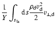
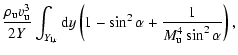
![\begin{figure}
\par\includegraphics[width=8.6cm,clip]{3898f3a.ps}\par\vspace{2mm...
...ps}\par\vspace{2mm}
\includegraphics[width=8.6cm,clip]{3898f3c.ps}
\end{figure}](/articles/aa/full/2006/43/aa3898-05/img221.gif)
![\begin{figure}
\par\hspace*{-2mm}\includegraphics[width=8.9cm,clip]{3898f4a.ps}\...
...ps}\par\vspace*{2mm}
\includegraphics[width=8.7cm,clip]{3898f4c.ps}
\end{figure}](/articles/aa/full/2006/43/aa3898-05/img243.gif)
![\begin{figure}
\par\hspace*{4mm}\includegraphics[width=8.1cm,clip]{3898f5a.ps}\p...
...e*{2mm}
\hspace*{2mm}\includegraphics[width=8.6cm,clip]{3898f5e.ps}
\end{figure}](/articles/aa/full/2006/43/aa3898-05/img257.gif)
![\begin{figure}
\par\includegraphics[width=8.4cm,clip]{3898f6a.ps}\par\vspace*{2mm}
\includegraphics[width=8.4cm,clip]{3898f6b.ps}
\end{figure}](/articles/aa/full/2006/43/aa3898-05/img258.gif)
![\begin{figure}
\par\includegraphics[width=8.1cm,clip]{3898f7a.ps}\par\vspace*{2mm}
\hspace*{2mm}\includegraphics[width=8cm,clip]{3898f7b.ps}\end{figure}](/articles/aa/full/2006/43/aa3898-05/img275.gif)
![\begin{figure}
\par\includegraphics[width=8cm,clip]{3898f8a.ps}\par\vspace*{2mm}...
...b.ps}\par\vspace*{2mm}
\includegraphics[width=8cm,clip]{3898f8c.ps}
\end{figure}](/articles/aa/full/2006/43/aa3898-05/img279.gif)

![\begin{figure}
\par\includegraphics[width=8cm,clip]{3898f10a.ps}\par\vspace*{2mm...
...b.ps}\par\vspace*{2mm}
\includegraphics[width=8cm,clip]{3898f10c.ps}\end{figure}](/articles/aa/full/2006/43/aa3898-05/img295.gif)
![\begin{figure}
\par\includegraphics[width=7.8cm,clip]{3898f11a.ps}\par\vspace{2mm}
\includegraphics[width=7.8cm,clip]{3898f11b.ps}
\end{figure}](/articles/aa/full/2006/43/aa3898-05/img298.gif)
![\begin{figure}
\par\hspace*{2mm}\includegraphics[width=8cm,clip]{3898f12a.ps}\pa...
...s}\par\vspace*{2mm}
\includegraphics[width=8.2cm,clip]{3898f12d.ps}
\end{figure}](/articles/aa/full/2006/43/aa3898-05/img306.gif)
![\begin{figure}
\par\includegraphics[width=8.1cm,clip]{3898f15a.ps}\par\vspace*{2...
....ps}\par\vspace*{2mm}
\includegraphics[width=8cm,clip]{3898f15c.ps}
\end{figure}](/articles/aa/full/2006/43/aa3898-05/img337.gif)
![\begin{figure}
\par\includegraphics[width=8.2cm,clip]{3898f16a.ps}\par\vspace*{2mm}
\hspace*{1mm}\includegraphics[width=8.2cm,clip]{3898f16b.ps}\end{figure}](/articles/aa/full/2006/43/aa3898-05/img338.gif)
![\begin{figure}
\par\includegraphics[width=8cm,clip]{3898f17a.ps}\par\vspace*{2mm}
\includegraphics[width=8.1cm,clip]{3898f17b.ps}
\end{figure}](/articles/aa/full/2006/43/aa3898-05/img340.gif)
![\begin{figure}
\par\includegraphics[width=8cm,clip]{3898f19a.ps}\par\vspace{2mm}
\includegraphics[width=8cm,clip]{3898f19b.ps}
\end{figure}](/articles/aa/full/2006/43/aa3898-05/img344.gif)