A&A 458, 953-963 (2006)
DOI: 10.1051/0004-6361:20065206
A. Costa1 - R. González2,3
1 - Instituto de Astronomía y Física del Espacio
(CONICET-Argentina)
2 -
Universidad
Nacional de General Sarmiento (UNGS)
3 - Departamento de Física (FCEyN-UBA-Argentina)
Received 14 March 2006 / Accepted 7 July 2006
Abstract
Aims. We study the modes and stability of non-isothermal coronal loop models with different intensity values of the equilibrium magnetic field.
Methods. We use an energy principle obtained via non-equilibrium thermodynamic arguments. The principle is expressed in terms of Hermitian operators and allow to consider together the coupled system of equations: the balance of energy equation and the equation of motion.
Results. We determine modes characterized as long - wavelength disturbances that are present in inhomogeneous media. This character of the system introduces additional difficulties for the stability analysis because the inhomogeneous nature of the medium determines the structure of the disturbance, which is no longer sinusoidal. Moreover, another complication is that we obtain a continuous spectrum of stable modes in addition to the discrete one.
Conclusions. We obtain a unique unstable mode with a characteristic time that is comparable with the characteristic life-time observed for loops. The feasibility of wave-based and flow-based models is examined.
Key words: standards - waves - Sun: corona
Stability is a crucial requirement for a model to produce realistic descriptions. Thus, different stability analyzed of solar structures can be found in the literature, generally restricted to special types of perturbations and specific equilibrium models. These includes, models that consider adiabatic configuration such as the ones analyzed via the classical criterion of Bernstein et al. (1958) or those that presuppose static equilibrium and analyze thermal stability. In the application of Bernstein's criterion, the adiabatic assumption implies that the energy balance equation is not required and thus dissipation is impossible. Also the assumption of static models is a strong, and often unjustified, restriction for open systems. Thus, a crucial question for any theoretical model is whether the much more common far-from-equilibrium states are stable, where the consideration of both thermal and mechanical coupled equations must be included.
A more realistic analysis of the stability of configurations represented by non-conservative equations was presented by Lerche & Low (1981). They proposed a Lagrangian principle in order to analyze quiescent prominences that can undergo thermal instabilities. However the non-self-adjoint character of the operators involved in the obtained principle makes the physical interpretation difficult.
In this paper we apply an energy
principle to analyze the stability of solar coronal loops. The
principle was obtained in a previous paper (Paper I: Costa et al.
2004; see also Sicardi et al. 2004; see also
Sicardi et al. 1991, 1989a,b, 1985) using a general
procedure of irreversible thermodynamics - based on firmly
established thermodynamic laws - that can be understood as an
extension of Bernstein's MHD principle to situations far from
thermodynamic equilibrium. This fact has the advantage that many
known results obtained by simpler criteria can be re-examined by
a direct comparison with our criterion, and that, as it is
obtained via a thermodynamic approach, allows a straightforward
physical interpretation. The principle associates stability with
the sign of a quadratic form avoiding non-self-adjoint
operators. Obtaining a self-adjoint operator is a requirement for
our principle to hold. When this is accomplished the calculus is
simplified. The self-adjoint character of an operator implies
that the eigenvalues
![]() are real. Hence stability
transitions always occur when
are real. Hence stability
transitions always occur when
![]() crosses zero, rather
than at particular points of the real axis where the real part of
the eigenvalue is different from zero, i.e. Re
crosses zero, rather
than at particular points of the real axis where the real part of
the eigenvalue is different from zero, i.e. Re
![]() ,
leading to an efficient formulation to test stability. Thus,
the symmetry considerations of the self-adjoint operators, the
fact that there is a diagonal form associated with these
operators, and that the Rayleigh-Ritz theorem states the
existence of a minimum eigenvalue, are important reasons to try to
maintain self-adjointness in the consideration of stability.
,
leading to an efficient formulation to test stability. Thus,
the symmetry considerations of the self-adjoint operators, the
fact that there is a diagonal form associated with these
operators, and that the Rayleigh-Ritz theorem states the
existence of a minimum eigenvalue, are important reasons to try to
maintain self-adjointness in the consideration of stability.
The theoretical modeling and the interpretation of observations of coronal loop systems deal, among others, with the discussion whether the propagating observed disturbances in loops and post-flare loops are waves or plasma flow.
Dynamical features of brightening coronal loops have been
traditionally interpreted as field-aligned flow of matter
generated by asymmetries in the energy input. Most classical
theoretical models have difficulties in determining the physical
conditions that make them compatible with observations. Both
static loops and steady state models - for the two classes of
temperatures models: hot (isothermal coronas with
![]() K) and cool (gradually increasing temperatures up to
K) and cool (gradually increasing temperatures up to
![]() K) - fail to provide a satisfactory explanation
for both the emission measure distribution and the Doppler shift
observations (Jordan 1980; Serio 1981; Craig
& McClymont 1978; Mariska 1984). Thus, this
suggests that in
traditional model scenarios radiative losses cannot
be compensated by thermal conduction. Therefore, other heating
mechanisms must be assumed (Aschwanden et al. 1999,
2000; Walsh & Galtier 2000). Also,
theoretical time-dependent models of individual loops where the
plasma evolves in response to a cyclical process of heating and
cooling of the flow have difficulties in fitting observations
(Klimchuk & Mariska 1988).
K) - fail to provide a satisfactory explanation
for both the emission measure distribution and the Doppler shift
observations (Jordan 1980; Serio 1981; Craig
& McClymont 1978; Mariska 1984). Thus, this
suggests that in
traditional model scenarios radiative losses cannot
be compensated by thermal conduction. Therefore, other heating
mechanisms must be assumed (Aschwanden et al. 1999,
2000; Walsh & Galtier 2000). Also,
theoretical time-dependent models of individual loops where the
plasma evolves in response to a cyclical process of heating and
cooling of the flow have difficulties in fitting observations
(Klimchuk & Mariska 1988).
The assumption of propagating disturbances associated with slow magnetoacoustic waves in high Alfvén speed media is also a field of investigation. Several wave-based models were developed to explain observations (Nakariakov et al. 2000; Tsiklauri & Nakariakov 2001). These authors suggest that - depending on the relative importance of dissipation by magnetic resistivity - upwardly propagating waves (of observed periods between 5-20 min) that decay significantly in the vicinity of the loop apex could explain the rarity of observational detection of downwardly propagating waves. However, upwardly propagating disturbances with non-decaying or even growing amplitudes were observed in coronal EIT plumes. Analytic models have shown that slow magnetoacoustic waves may be trapped and nonlinearly steepened with height, providing a possible interpretation of this phenomenon (Ofman et al. 1999).
However, due to the intensity of the flaring, the plasma dynamic of flare loops is generally associated with flows rather than with waves. In fact, systematic intensity perturbations in post-flare loops can suggest that they are the result of evaporation-condensation cycles caused by the efficient heating of the flaring plasma from the chromosphere. Thus, chromospheric evaporation seems to be the main initial matter inflow source for flare loops. De Groof et al. (2004) analyzed an off-limb half loop structure from an EIT shutterless campaign and gave arguments to reject the slow magnetoacoustic description and to support the flowing/falling plasma one. Nevertheless, these authors admit that the wave theory cannot be excluded yet.
Other authors have suggested that a combination of phenomena can be at the basis of a better interpretation. Alexander et al. (1998) examined 10 flares and concluded that plasma turbulence could be the source of the observed intensity changes rather than hydrodynamic flows such as chromospheric evaporation. They pointed out that it cannot be excluded that there is a degree of "gentle evaporation'' occurring early in the event with associated hard X-ray emission below their threshold of detection. A series of more recent papers (Tsiklauri et al. 2004a-c) that combine theoretical and observational analysis showed that oscillations in white, radio and X-ray light curves observed during solar and stellar flares may be produced by slow standing magnetoacoustic modes of the loops. They found that a transient heat deposition at the loop bottom - or at the apex - leads to a posterior up-flow evaporation of material of the order of a few hundreds of km s-1. During the peak of the flare, the simulations showed that a combined action of heat input and conductive and radiate losses could yield an oscillatory pattern with typical amplitudes of up to a few tens of km s-1. Then, a cooling phase of plasma draining with velocities of the order of hundreds of km s-1 occurs. The numerical quasi-periodic oscillations in all the physical quantities, that resemble observational features, were interpreted as being produced by standing sound waves caused by impulsive and localized heating.
In previous papers (Borgazzi & Costa 2004; Costa & Stenborg 2004) one of us developed a diagnostic observational method to describe loop intensity variations, both in space and time, along coarse-grain loop structures. We find that none of the arguments leading to the determination of whether waves or flow models can better fit observations was conclusive. Some of our results suggested wave-based model interpretations i.e. the periodic behaviour of the disturbances observed, the almost constant speed of some brightening features and the fact that the estimated speeds were not higher that the sound speed in the coronal loops. However, as we mentioned, the period behaviour can also be attributed to flows (Gómez et al. 1990; De Groof et al. 2004). Also, even when the calculated speeds were not greater than the sound ones, some of the velocity patterns were far from being constant and their values were comparable to the free-fall case.
Another open question is the relation between the loop's coronal dynamics and the physical conditions on the chromospheric bases. Borgazzi & Costa (2004) found a longitude of chromospheric coherence that characterizes the behaviour of a whole loop-system of evolving coronal-isolated filaments. This description is in accordance with limit-cycle models that require that the triggering mechanism of the dynamics is located at the bottom of the structure giving rise to the observed similar coronal conditions of the isolated filaments. Another aspect that deserves attention is whether it is physically possible that the periodicity observed could be related to, or could be the consequence of propagating magnetoacoustic modes from the chromosphere that have suffered distortion due to the dispersing media.
Other point that is under debate is the thermal structure of the loops. Loop observations with TRACE (Transition Region and Coronal Explorer, Handy et al. 1999) suggest that hot coronal loops are isothermal and more dense than the predictions of static loop models. However this scenario is not conclusive and other interpretations are possible. Reale & Peres (2000) showed that bundles of thin strands, each one behaving as a static loop, with its characteristic thermal structure, convoluted with the TRACE temperature response could appear as a single almost isothermal loop. A wide range of configurations can be proposed to fit observations. The fact that images form a compound of complex integrated time-varying data that are not easy to resolve is at the basis of this difficulty. The loops under analysis are surrounded by other structures that usually intersect them along the line of sight and the change of the brightening of the loops is also affected by background emission. Thus, efforts are made to produce observational and theoretical results of coronal loop dynamics.
The aim of this paper is to investigate whether the propagating observed disturbances in loops are waves or plasma flow and their thermal structure. Non-isothermal loops are traditional candidates for Hopf instabilities with cycles of flow evaporating and condensing, thus the analysis of frequencies and mode structures can provide insight into a possible wave model interpretation of these types of configurations. We consider the stability analysis as the leading criterion to select possible theoretical wave models. The fact that a number of non-linear equilibria are possible due to the open character of the systems makes it necessary to consider both thermal and mechanical stability in a coupled way.
The thermodynamics of irreversible processes is described in terms of phenomenological relations between conjugate pairs of thermodynamic variables: the flows and the forces that cause them. The linear thermodynamic approximation treats small deviations from the equilibrium state by including fluctuations in the neighborhood of this state. It describes the behaviour of the system around the equilibrium state or around a non-equilibrium stationary one that is linearly close to it.
If the system is isolated, as is stated by the second law of
thermodynamics, the entropy grows exponentially up to its maximum
value. That the system is in an open-near-equilibrium state
means that energy and matter is exchanged with the neighbors and
the entropy of the system is not necessarily positive. Even when
the entropy produced in the system's interior, due to irreversible
processes, is never negative, a negative flow of entropy produced
by the exchange of matter and energy can make the system remain
indefinitely in a near-equilibrium state. These states are known
as stationary states and a coherent dynamic of the system could
last if sufficient negative entropy flow is provided to it. Thus,
the criterion that states the stability of this stationary state
gives insight into the dynamic structures that can be found in
nature. These stationary states are also known as detailed
balanced. As Onsager pointed out (1931), the balance
consists of the compensation between the fluctuations and
dissipation produced by the flows and forces that have a
microscopic reversible character near the thermodynamic
equilibrium. The empirical relations between flows and forces are
linear and related by the so-called resistance matrix ![]() that is symmetric and positive definite. Its
symmetric character is guaranteed by the principle of microscopic
reversibility and its positive definiteness by the proximity of
the reference state to the thermodynamic equilibrium, where the
entropy has a maximum.
that is symmetric and positive definite. Its
symmetric character is guaranteed by the principle of microscopic
reversibility and its positive definiteness by the proximity of
the reference state to the thermodynamic equilibrium, where the
entropy has a maximum.
However, there is no continuity between linear and nonlinear
thermodynamical processes. When the system is beyond the immediate
neighborhood of the stationary state the nonlinearities become
visible. Instabilities that cause dynamic transitions in open
systems are responsible for the qualitative difference between
linear and nonlinear thermodynamics. Therefore, dynamic
cooperative phenomena can only arise in nonlinear thermodynamics.
Thus, nonlinear thermodynamics is related to the stability
properties of non-equilibrium stationary states, where the linear
relation between flows and forces can become state dependent (i.e. ![]() is not necessarily a symmetric positive definite
matrix), and the problem of having a thermodynamic theory to
provide a general criterion for the stability of the system - which
is not evident through the integration of the variational
equations - becomes a fundamental point. Non-linear thermodynamics
is the extension of the linear theory to situations far from
thermodynamic equilibrium where the relaxation of the processes to
a steady state of non-equilibrium (nonlinear state) is not assured
and requires a stability analysis (Glansdorff & Prigogine
1971; Keizer 1976; Graham 1978; Lavenda
1993, 1987).
is not necessarily a symmetric positive definite
matrix), and the problem of having a thermodynamic theory to
provide a general criterion for the stability of the system - which
is not evident through the integration of the variational
equations - becomes a fundamental point. Non-linear thermodynamics
is the extension of the linear theory to situations far from
thermodynamic equilibrium where the relaxation of the processes to
a steady state of non-equilibrium (nonlinear state) is not assured
and requires a stability analysis (Glansdorff & Prigogine
1971; Keizer 1976; Graham 1978; Lavenda
1993, 1987).
In Paper I we showed how to obtain the variational principle from the equations that describe the dynamics of the system of interest. The method consists of obtaining a Lyapunov function, also known as generalized potential, that represents the mathematical expression of the stability conditions. This function is determined by the analysis of the thermodynamic properties of the system linearized around a non-linear stationary state also called non-linear equilibrium state. The equations governing the dynamics are written as a system of two coupled equations: the balance energy equation and the equation of motion. Thus, the perturbation analysis around a stationary state is performed considering a variable state vector of four independent components: the three space component displacement and the temperature variation. Once the linearization is done, the Lyapunov function can be immediately obtained by inspection of the resulting expression written in a compact matrix form. Each of the matrices of the compact expression are linear operators (that could include spatial derivatives) and have a clear physical interpretation that is given by its role in the equation. The matrix that multiplies the second time derivative of the perturbation is associated with the inertia of the system, the one that multiplies the first time derivative of the perturbation is associated with dissipation and the one that multiplies the perturbation itself is associated with potential forces over the system. The principle is subject to physically reasonable requirements of hermiticity and antihermiticity over the matrices. For a more detailed presentation see Paper I and the references presented there.
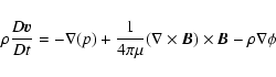
The specific model we analyze is taken to be composed of
a magnetohydrodynamic ideal plasma (i.e. with infinite electrical
conductivity
![]() ). The fundamental ideal
magnetohydrodynamic equations to be considered are as follows. The
mass conservation equation,
). The fundamental ideal
magnetohydrodynamic equations to be considered are as follows. The
mass conservation equation,
The linearization procedure is performed by replacing
![]() ,
T=T0+T1,
B=B0+B1 and
,
T=T0+T1,
B=B0+B1 and
![]() in the last
equations, and assuming hydrostatic conditions for the equation of
motion. Thus,
in the last
equations, and assuming hydrostatic conditions for the equation of
motion. Thus,
![]() and
and
![]() where
where ![]() is the
perturbation around the equilibrium of the equation of motion (the
stationary state), also
is the
perturbation around the equilibrium of the equation of motion (the
stationary state), also
![]() and
and
![]() .
Using the relation
.
Using the relation
![]() in Eqs. (1) and (3), the corresponding linearized equations (Eqs. (8)-(12)) are:
in Eqs. (1) and (3), the corresponding linearized equations (Eqs. (8)-(12)) are:
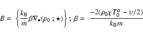
![\begin{displaymath}A=-\left[c\nabla \cdot \left(T_{0}^{\frac{5}{2}}\nabla
_{\par...
...frac{\rho _{0}^{2}}{m^{2}}\chi \alpha
T_{0}^{\alpha -1}\right] \end{displaymath}](/articles/aa/full/2006/42/aa5206-06/img66.gif)
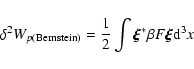
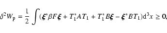
Following Paper I the resulting energy principle is:
For the non-dissipative cases, last expression reduces to the
well-known Bernstein MHD energy principle
We are interested in analyzing the stability of non-homogeneous loops. This is, loops with inhomogeneous distributions of plasma density and temperatures. This character of the system poses additional difficulties for the stability analysis because the inhomogeneous nature of the medium determines the structure of the disturbance which is no longer sinusoidal, making the traditional normal mode analysis useless for this treatment. Moreover, there may exist a continuous spectrum of stable modes besides the discrete one. As a first order approximation we neglect the effect of gravitational stratification and thus confine the analysis to characteristic spatial scales lower than the pressure scale height in the solar corona. In order to analyze the stability and to obtain the frequencies and modes the physical quantities in Eqs. (17) and (18) must be calculated along the loop structure.
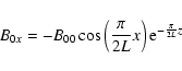
In order to determine an equilibrium configuration we assume
force-free equations due to the fact that in plasma with low
![]() (gas pressure over the magnetic pressure) the
pressure gradient can be neglected in comparison to the Lorentz
force. The coronal arcade is obtained from the equations
(gas pressure over the magnetic pressure) the
pressure gradient can be neglected in comparison to the Lorentz
force. The coronal arcade is obtained from the equations
| |
Figure 1:
Schematic figure of the magnetic arcade with
|
| Open with DEXTER | |
The thermal equilibrium is obtained from Eq. (7) with L=0(in Eq. (6)). Thus expressions
![]() satisfies the two
relations
satisfies the two
relations
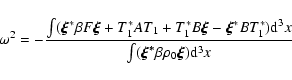
In order to calculate the stability and structure modes the
general perturbation expression along the equilibrium loop is
written
In order to calculate modes and frequencies we followed the
schematic procedure described in Paper I and in Galindo Trejo
(1987). We used a symbolic manipulation program to integrate
the equations.
![]() and the perturbations were
expanded in a three dimensional-Fourier basis that adjusts to
border conditions. Thus, a quadratic form for
and the perturbations were
expanded in a three dimensional-Fourier basis that adjusts to
border conditions. Thus, a quadratic form for
![]() was obtained and was minimized with the Ritz variational
procedure. A matrix discrete eigenvalue problem subject to a
normalization constraint was obtained. The procedure is equivalent
to solving Eq. (18) of our modified principle. Once the modes
are obtained, the stability condition of Eq. (17) for the
generalized potential energy:
was obtained and was minimized with the Ritz variational
procedure. A matrix discrete eigenvalue problem subject to a
normalization constraint was obtained. The procedure is equivalent
to solving Eq. (18) of our modified principle. Once the modes
are obtained, the stability condition of Eq. (17) for the
generalized potential energy:
![]() must be
corroborated. The following values were used for the numerical
calculation of the modes
must be
corroborated. The following values were used for the numerical
calculation of the modes
Our main concern was to know whether the
magnetic configuration of equilibrium could be stable under
linear perturbations. For non homogeneous configurations it is
well known that the stable eigenvalues can have continuous
spectra while the unstable ones have a discrete spectrum (see
Freidberg 1982; or Priest 1982). If the
resulting mode components have a characteristic wavelength of the
order of the equilibrium structure, the non-homogeneous character
of modes could determine, for the stable modes, a continuous
spectrum. Thus, in this case, the traditional normal mode
analysis gives only a rough description because one of the
consequence of the existence of the continuum is that an
accumulation of discrete eigenvalues can take place at either
boundary, generally at
![]() or
or
![]() ,
indicating the presence of a continuum stable spectrum. Note that
as the basis used is discrete, the spectrum is necessarily
discrete. However, the additional evaluation of the generalized
potential energy provides the correct unstable modes and gives
an approximate value of the most probable stable period when the smaller
,
indicating the presence of a continuum stable spectrum. Note that
as the basis used is discrete, the spectrum is necessarily
discrete. However, the additional evaluation of the generalized
potential energy provides the correct unstable modes and gives
an approximate value of the most probable stable period when the smaller
![]() is not located at the boundaries.
is not located at the boundaries.
We used different values for k: k=0, k=0.5 and k=10 (k is the wavenumber associated with the perturbation component transverse to the plane that contains the magnetic configuration). We also calculated the frequencies and modes for two different values of the magnetic field: B00=11 G and B00=100 G.
Table 1: Periods associated with the unstable and stable eigenvalues (minutes) for B00=11 G.
Table 2: Periods associated with the unstable and stable eigenvalues (minutes) for B00=100 G.
Tables 1 and 2 show the eigenvalues (periods) associated with the different modes for the cases B00=11 G and B00=100 G respectively, considering k=0 and obtained by solving Eq. (18). We obtained 12 eigenfrequencies and 12 eigenmodes for each of the magnetic field values i.e. we used a three-component expansion and a four-component perturbation vector. We evaluated the mode behaviour for| |
Figure 2:
Mode components corresponding to the first mode
P1=36.3 min for the cases: a) |
| Open with DEXTER | |
| |
Figure 3:
Mode components corresponding to the second
modes:
a) |
| Open with DEXTER | |
From the analysis of the table data we can conclude: 1) for each
of the two investigated magnetic values we have three complex
values of ![]() and six real ones; 2) in the two magnetic
field cases the eigenvalues of the first mode are the same; 3) in
all the other cases the eigenvalues with
B00=100 G are
almost an order of magnitude smaller than the corresponding values
of B00=11 G; 4) the series of eigenvalues is such that it
could be possible that the stable periods accumulate at
and six real ones; 2) in the two magnetic
field cases the eigenvalues of the first mode are the same; 3) in
all the other cases the eigenvalues with
B00=100 G are
almost an order of magnitude smaller than the corresponding values
of B00=11 G; 4) the series of eigenvalues is such that it
could be possible that the stable periods accumulate at ![]() ,
thus the definite stability characterization is
subject to the evaluation of the generalized potential energy of
the
modes.
,
thus the definite stability characterization is
subject to the evaluation of the generalized potential energy of
the
modes.
We analyzed the structure of the modes with complex values of ![]() as they are possible candidates for instability
(Freidberg 1982). We noted that in the two first
modes the component that is tangent to the magnetic field
as they are possible candidates for instability
(Freidberg 1982). We noted that in the two first
modes the component that is tangent to the magnetic field
![]() is greater than the component
is greater than the component
![]() that
is normal to it. This can be seen from Figs. 2 and 3 where
that
is normal to it. This can be seen from Figs. 2 and 3 where ![]() and
and ![]() are shown for the
cases: B00=11 G and
B00=100 G respectively, also using
k=0. The third mode (see Fig. 4) has comparable
values of
are shown for the
cases: B00=11 G and
B00=100 G respectively, also using
k=0. The third mode (see Fig. 4) has comparable
values of
![]() and
and
![]() .
.
The fact that for the first mode the two values of B00 give
the same time eigenvalue
![]() min indicates independence from the magnetic structure. This is
consistent with the relative values between the two components in
the two B00 cases:
min indicates independence from the magnetic structure. This is
consistent with the relative values between the two components in
the two B00 cases:
![]() (see Fig. 2).
Thus, these magnetoacoustic modes are
more of the acoustic type
(see Fig. 2).
Thus, these magnetoacoustic modes are
more of the acoustic type
![]() than of
the Alfvén type, i.e.
than of
the Alfvén type, i.e.
![]() (see
Fig. 5). Also, the obtained period is included in
a range (
(see
Fig. 5). Also, the obtained period is included in
a range (
![]() min) where MHD slow acoustic modes are
expected (Aschwanden 2004).
min) where MHD slow acoustic modes are
expected (Aschwanden 2004).
Figure 3 shows the second mode for B00=11 G and
B00=100 G respectively. Also for both cases the
![]() perturbation is greater than the normal
perturbation
perturbation is greater than the normal
perturbation
![]() by an order of magnitude.
by an order of magnitude.
Figure 4 show the superposition of ![]() and
and ![]() for the third modes corresponding to P=4.3 min,
B00=11 G and P=0.5 min,
B00=100 G respectively. Note
that in these cases, when the component
for the third modes corresponding to P=4.3 min,
B00=11 G and P=0.5 min,
B00=100 G respectively. Note
that in these cases, when the component ![]() is relevant,
resembling an Alfvén wave, the relation between the eigenvalues
(periods) of the different magnetic fields is
is relevant,
resembling an Alfvén wave, the relation between the eigenvalues
(periods) of the different magnetic fields is
![]() ,
in accordance with the relation between the two values
of
,
in accordance with the relation between the two values
of
![]() and with the corresponding
values of the Alfvén velocities of the medium
and with the corresponding
values of the Alfvén velocities of the medium
![]() .
.
| |
Figure 4:
|
| Open with DEXTER | |
| |
Figure 5:
Schematic classification of fast and slow magnetoacoustic waves. |
| Open with DEXTER | |
Figure 5 gives a schematic classification of fast
and slow magnetoacoustic waves from where we can analyze the
behaviour of the modes. The first mode corresponds to
![]() and as its eigenvalue is independent of the magnetic
field it gives a slow magnetoacoustic mode. The third mode
corresponds to
and as its eigenvalue is independent of the magnetic
field it gives a slow magnetoacoustic mode. The third mode
corresponds to
![]() and as
and as
![]() it looks like a fast magnetoacoustic mode (Priest
1982).
it looks like a fast magnetoacoustic mode (Priest
1982).
Then, in order to establish the final unstable modes we integrated Eq. (17) for each of the normal modes, i.e., the integrand is the generalized potential energy density.
Figure 6 shows the generalized potential energy density as a
function of the independent variable x for the three first
modes (see Table 1), and for the most stable one which was P4.
We show the case B00=11 G, the case
with
B00=100 G has the same functional dependence. Table 3
shows the eigenvalues and the potential energy for the modes with
complex eigenvalues and for the most stable one. Note that, even
when ![]() has complex values for the three first modes, as
has complex values for the three first modes, as
![]() is positive in the second and third case, the
P1 = 36.3 min mode is the only unstable one. The fact that,
on the contrary to what happens with the first mode, the other
modes with complex
is positive in the second and third case, the
P1 = 36.3 min mode is the only unstable one. The fact that,
on the contrary to what happens with the first mode, the other
modes with complex ![]() seemed to accumulate at the origin is
an indication of non-real unstable modes.
seemed to accumulate at the origin is
an indication of non-real unstable modes.
![\begin{figure}
\par\includegraphics[width=5cm,clip]{5206fg6a.eps}\par\vspace*{2m...
...par\vspace*{2mm}
\includegraphics[width=5cm,clip]{5206fg6d.eps}
\end{figure}](/articles/aa/full/2006/42/aa5206-06/img163.gif) |
Figure 6:
Generalized potential energy density as a function of x for the modes a) P1=36. min with
|
| Open with DEXTER | |
Table 3: Potential energy (non dimensional) of the three first modes (complex eigenvalues) and the fourth (most stable mode) B00=11 G.
Figure 7 shows the structure of the components ![]() and
and ![]() for the most stable mode P4 and for the
two cases: B00=11 G and
B00=100 G. Note that
for the most stable mode P4 and for the
two cases: B00=11 G and
B00=100 G. Note that
![]() and that
and that
![]()
| |
Figure 7:
components of the most stable periods
a) |
| Open with DEXTER | |
The mode structure of the stable eigenvalues can also be
compared with recent results from the literature. Magnetoacoustic
oscillations of the fast kink type have been studied theoretically
(Edwin & Roberts 1983) and directly observed in EUV wavelengths with TRACE
(an updated review of theoretical and observational results in
Aschwanden 2004, and references therein).
The observations are usually modeled by cylinders with a surface
boundary representing coronal loops. The dispersion relation is
obtained matching the internal and external MHD solutions via the
requirement of continuity of pressure and perpendicular velocity.
As in our model, the observed kink-mode oscillations correspond to
the long-wavelength regime. In coronal conditions the magnetic
field is almost equal inside and outside of the loop and the kink
oscillation speed is almost the Alfvén one depending on the
ratio of external and internal density values, i.e., outside and
inside the loop. On the contrary, our model is performed by
perturbing a magnetic arcade, without considering a cylinder with
different inside and outside conditions. In eleven observational
kink-mode oscillations from which the magnetic field of the events
can be inferred were obtained by Aschwanden et al. (2002)
and (2003).
The
comparison of our stable mode data Pi>1 in the
B00=11 G case is in good agreement with the kink-mode observational results.
The period range (see Table 1), the magnetic strength
(B00=11 G) and the wave speed (Alfvén speed) fit the
observations for similar loop densities and loop lengths. Also,
the stable modes Pi
>1 with
B00=100 G (see Table 2) have periods that are
comparable with the expected range of fast sausage-mode periods
(
![]() s) and wave speeds of the order of the Alfvén
speed (Aschwanden 2004). However - even when a more
precise comparison requires a modeling that takes into account
differences between external and internal conditions - it is worth
investigating whether these type of modes could be associated with
more intense magnetic fields in comparison to the associated
kink-mode magnetic fields. This will be attempted in future work.
s) and wave speeds of the order of the Alfvén
speed (Aschwanden 2004). However - even when a more
precise comparison requires a modeling that takes into account
differences between external and internal conditions - it is worth
investigating whether these type of modes could be associated with
more intense magnetic fields in comparison to the associated
kink-mode magnetic fields. This will be attempted in future work.
A main result regarding stability is that the characteristic time
![]() min in which the instability grows is large enough
to guarantee a relative permanence of the structure before it
fades away:
min in which the instability grows is large enough
to guarantee a relative permanence of the structure before it
fades away:
![]() ;
where
;
where
![]() is the typical
characteristic time in which loops seem stable (see Costa &
Stenborg 2004). Thus, even when the non-linear
stationary configuration of Fig. 1 is unstable it
lasts long enough for the observations to be made. Moreover, we
confirm that the dynamic brightenings usually observed
could be due to magnetoacoustic
waves i.e. the perturbations have short periods in comparison
with the time that instability occurs:
P4= 3.4 min and
P4=0.36 min satisfy
is the typical
characteristic time in which loops seem stable (see Costa &
Stenborg 2004). Thus, even when the non-linear
stationary configuration of Fig. 1 is unstable it
lasts long enough for the observations to be made. Moreover, we
confirm that the dynamic brightenings usually observed
could be due to magnetoacoustic
waves i.e. the perturbations have short periods in comparison
with the time that instability occurs:
P4= 3.4 min and
P4=0.36 min satisfy
![]() .
.
Thus, even when further calculation is needed in order to adjust the characteristic times, it seems that wave-based models could be able to describe the scenario of non-isothermal coronal loops for sufficiently short times comparable with the characteristic time in which the instability grows and the structure fades away. A more speculative argument about the relation between wave-based models and flow-based ones is given in the conclusions.
We investigated - via a thermodynamic energy principle - the stability of a coronal inhomogeneous loop model in a non-linear equilibrium state, i.e. a given thermal and magnetic equilibrium configuration. We also obtained the frequencies and their associated modes. The perturbation chosen was of the general type described by Eq. (31) which allowed the study of a more complex mode structure with coupled thermal and mechanical displacements from the equilibrium state. We used a three-component Fourier basis expansion on the independent coordinate x to characterize the unstable modes. We obtained three complex eigenvalues and six real ones with their corresponding eigenvectors for each of the magnetic field values B00 analyzed. The other three modes were discarded. The definite stability condition of the modes is given by integrating the generalized potential energy density of Eq. (17), allowing the interpretation of long-wavelength disturbances that are present in inhomogeneous media.
| |
Figure 8: Thermal perturbation (T1 component) for the cases: a) P=36 min; B00=11 G b) P=36 min; B00=100 G. |
| Open with DEXTER | |
| |
Figure 9:
Schematic description of the unstable
mode superimposed on the magnetic structure. At a definite
phase the perturbation is always positive, it grows until
it reaches |
| Open with DEXTER | |
![\begin{figure}
\par\includegraphics[width=5cm,clip]{5206fg10a.ps}\par\vspace*{2mm}
\includegraphics[width=5cm,clip]{5206fg10b.ps}
\end{figure}](/articles/aa/full/2006/42/aa5206-06/img182.gif) |
Figure 10: The curve formed by the resulting component perturbations in the vector space of perturbations for a) B00=11 G and b) B00=100 G. |
| Open with DEXTER | |
Acknowledgements
This paper is dedicated to the memory of our Professor and guide Constantino Ferro Fontán, and also to the memory of our colleague and friend Aníbal Sicardi Schifino.
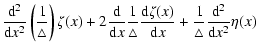
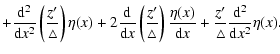
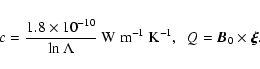
The following equations and relations are needed in order to
obtain Eq. (33)

![\begin{displaymath}\frac{k_{\rm B}}{m(\gamma-1)}[\rho_{0}\dot{T_{1}}-(\gamma-1)T_{0}
\nabla\cdot(\rho_{0}\dot{\vec{\xi}})]-AT_{1}+B\vec{\xi}=0
\end{displaymath}](/articles/aa/full/2006/42/aa5206-06/img65.gif)
![\begin{displaymath}\delta^{2} S = \frac{ 1}{ 2}\int \left[\-\dot{\vec{\xi^{*}}}\...
...{ \vec{\xi^{*}} \beta F
\vec{\xi}} \right] {\rm d}^{3}x \geq 0
\end{displaymath}](/articles/aa/full/2006/42/aa5206-06/img73.gif)
![\begin{displaymath}z= z_{\rm t}+\frac{2L}{\pi}\ln\left[\cos\left(\pi
\frac{x}{2L}\right)\right]
\end{displaymath}](/articles/aa/full/2006/42/aa5206-06/img86.gif)

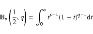
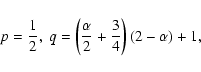
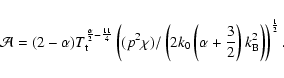
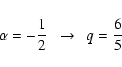
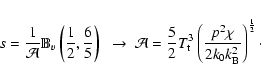
![$\displaystyle {\int_{T_{0}}}^{T}
k_{0}T'^{\frac{5}{2}}\left[\frac{\rho^{2}}{m^{2}}Q(T')-H_{0}\right]
{\rm d}T'$](/articles/aa/full/2006/42/aa5206-06/img95.gif)
![\begin{displaymath}\left[\frac{{\rm d}T}{{\rm d}s}\right]^{2}=\frac{p^{2}\chi}{2...
...} \left[1 - \left(\frac{T}{T_{\rm t}}\right)^{2-\alpha}\right]
\end{displaymath}](/articles/aa/full/2006/42/aa5206-06/img103.gif)

![\begin{displaymath}\frac{{\rm d}T}{{\rm d}s}=\mathcal{A}\left[\frac{{\rm d}\mathbb{B}_{v}}{{\rm d}v}\frac{{\rm d}v}{{\rm d}T}\right]^{-1}\cdot
\end{displaymath}](/articles/aa/full/2006/42/aa5206-06/img109.gif)
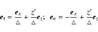
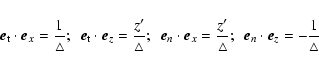
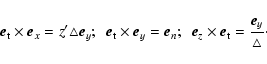
![\begin{displaymath}\vec{\xi}=[\zeta(x)
\vec{e}_{\rm t}+\eta(x)\vec{e}_{n}+\xi_{y}(x)\vec{e}_{y}]{\rm e}^{{\rm i}ky}
\end{displaymath}](/articles/aa/full/2006/42/aa5206-06/img110.gif)

![$\displaystyle \hspace*{2mm}-k \beta T_{0} \xi_{y}\left (
\frac{{\rm d}\rho_{0}}{{\rm d}x} f-k\rho_{0}\xi_{y} \right ) \left. \right.
{\Bigg ]}$](/articles/aa/full/2006/42/aa5206-06/img114.gif)
![$\displaystyle \hspace*{2mm} + \left ( \frac{{\rm d}}{{\rm d}x}\left(\frac{\vec{...
...eta}{{\rm d}x}-k\frac{z'}{\triangle}\vec{B}_{0}\xi_{y})^{2}
{\Bigg )} {\Bigg ]}$](/articles/aa/full/2006/42/aa5206-06/img117.gif)
![$\displaystyle \hspace*{2mm}
-\beta \left [ \frac{1}{\triangle}\frac{{\rm d}\rho...
...}x}\eta\frac{{\rm d}T_{1}}{{\rm d}x}+k\rho_{0}\xi_{y}
T_{1} \right ] {\Bigg \}}$](/articles/aa/full/2006/42/aa5206-06/img121.gif)
![\begin{displaymath}\vec{\xi}=\left[f(\zeta,\eta)
\vec{e}_{x}+{\rm i} \xi_{y}\vec{e}_{y}
+g(\zeta,\eta)\vec{e}_{z}\right]{\rm e}^{{\rm i}ky}
\end{displaymath}](/articles/aa/full/2006/42/aa5206-06/img192.gif)