A&A 458, 597-608 (2006)
DOI: 10.1051/0004-6361:20054666
L. N. Georgiev1,2 - D. J. Hillier2 - J. Zsargó2
1 - Instituto de Astronomía, UNAM, CD. Universitaria,
Apartado Postal 70-264, 04510 México DF, México
2 - Physics and Astronomy Department, University of Pittsburgh, 3941 O'Hara Street, Pittsburgh PA 15260, USA
Received 8 December 2005 / Accepted 28 June 2006
Abstract
Aims. This paper describes a code which is capable of modeling axisymmetric stellar winds.
Methods. At present the code uses a short characteristic technique for the continuum transfer, while bound-bound transitions are treated using the Sobolev approximation. The simultaneous solution of the transfer equations, and the equations of statistical equilibrium, is achieved by a combination of preconditioning and linearization.
Results. Extensive tests were performed which show that, in the extreme conditions of gray opacity or spherical symmetry, the code performs similar to other established codes. Simple 2D tests have been undertaken which confirm the performance of the code, and serve to illustrate simple effects that can occur in axisymmetric stellar winds. The code has been designed with flexibility in mind, with the radiation transport section treated, as far as possible, distinctly from the solution of the statistical equilibrium and energy balance equations. This will facilitate the inclusion of other transport solvers, and the treatment of more complex geometries.
Key words: stars: atmospheres - stars: early-type - stars: winds, outflows - line: formation - radiative transfer
Massive stars are one of the principal sources of heavy elements in galaxies. These stars have stellar winds which expel the outer layers of the star, mixing their material with the interstellar gas. Recent developments in the theory of stellar evolution (Maeder & Meynet 2003) show that rotation has a major influence on the evolution of a star and the chemical composition of its atmosphere. Further, rotation can deform the star, deviating its atmosphere and wind from spherical symmetry (Bjorkman & Cassinelli 1993; Owocki et al. 1994). The influence of deviations from spherical geometry on observed spectra are complicated, and their effect on results obtained using quantitative 1D detailed modeling is unclear. Although difficult, multi-dimensional models are essential for reliable and quantitative analysis of real stars.
The need for multi-dimensional models also arises in interacting binary systems. In O star binary systems, wind-wind collisions occur and these can have a substantial effect on the observed wind spectra (Hill et al. 2002). The analysis of the wind eclipses in WR+O binaries (Auer & Koenigsberger 1994) is a promising tool for studying the wind structure. However the structure of the primary wind is influenced by the radiation field of the secondary star, and thus its correct application requires 2D modeling. The Hatchett-McCray effect (Hatchett & McCray 1977) is another example of an interaction between stars in a binary system, and for which correct interpretation is impossible with 1D codes. Even radial velocity curves of massive binaries are affected by profile changes due to the deviation from spherical symmetry, and these changes need to be taken into account if accurate mass ratios are to be obtained.
The importance of multi-dimensional modeling has been known since the beginning of computer-based stellar atmosphere modeling. But the straight forward application of 1D techniques to 2D problems was not possible and the development of codes was delayed. Several important developments have now made progress possible. These include the dramatic increase in computational power, the availability of the necessary atomic data, and new computational techniques. For example, Mihalas et al. (1978) and Auer & Paletou (1994) introduced the short characteristic method for solution of the equation of radiative transport (ERT). The method is flexible and can be generalized for different geometries and dimensions (e.g., van Noort et al. 2002). Olson et al. (1986) introduced the Approximate Lambda Operator (ALO) to overcome the slow convergence of the usual Lambda iteration. The method combines the simplicity of the Lambda iteration with good convergence properties. Variants of this technique, which use linearization, have also been shown to be extremely useful for construction of 1D non-LTE model atmospheres (Hillier 1990; Hubeny & Lanz 1995). Finally, Rybicki & Hummer (1991) combined the ALO with preconditioning of the statistical equilibrium equations (SEE) which replaces the linearization technique.
Other codes, and techniques, are being developed to perform multi-dimensional radiative transfer. For example, Monte-Carlo techniques have also been utilized to perform multidimensional radiative transfer calculations. Both Juvela (1997) and Park & Hong (1998) have used Monte-Carlo techniques to model CS molecule spectra produced by clumpy cloud models. Monte-Carlo codes have also been extensively applied to the study SEDs of protostars (Whitney et al. 2003b,a). Despite the use of the MC approach, techniques have been developed that allow the temperature structure of the envelope to be solved for (Lucy 1999a; Bjorkman & Wood 2001). Most, if not all, the Monte-Carlo codes use the Sobolev approximation for the line transfer. A major proponent of the Monte-Carlo technique is Lucy, who has devoted considerable effort to its development (e.g., Lucy 1999a,b, 2003).
Given the complexity of non-LTE multi-dimensional radiative transfer, and the wide variety of astrophysical situations where they can be applied, it is important to develop independent codes and techniques. With such independent codes, issues of accuracy and efficiency can be addressed. Importantly, the absolute accuracy of results can be be discerned by a detailed comparison between results obtained using independent codes.
In this paper we describe an early version of a non-LTE radiative transfer code that can be used to undertake detailed spectral analysis in 2D, and in particular spectral analysis of stars with non-spherical stellar winds. The code utilizes several of the numerical techniques mentioned previously. It solves self consistently the ERT simultaneously with the system of SEE and the energy conservation equation. At present we limit ourselves to models with axisymmetry although we allow for the influence of rotation. The solution of the continuum ERT is similar to the one described by Busche & Hillier (2000).
The paper is organized as follows. Section 2 describes the coordinate system and the method used to solve the ERT. In Sect. 3 we discuss the solution of the system of statistical equilibrium equations, the use of the Sobolev approximation for bound-bound transitions, and the electron thermal balance (ETB). The technique we use for the simultaneous solution of the ERT, SEE, and ETB is also discussed. Section 4 presents a comparison of 1D models with those of CMFGEN, and detailed results for simple 2D models.
The solution of the radiative transfer equation follows closely the method described by Busche & Hillier (2000). For a more consistent description of the code we briefly summarize the main ideas.
The parameters of the gas are described in two coordinate systems.
One is a Cartesian system (x y z) with the z axis
along the symmetry axis. The second system is spherical (
![]() ), defined so
that the angle
), defined so
that the angle ![]() is measured
from the z axis (Fig. 1). Due to the symmetry, variables describing the conditions of the gas
and the radiation do not depend on
is measured
from the z axis (Fig. 1). Due to the symmetry, variables describing the conditions of the gas
and the radiation do not depend on ![]() .
In the spherical system we define a
grid
.
In the spherical system we define a
grid
![]() (where
(where
![]() and
and
![]() ). As usual,
ri > ri+1 and
). As usual,
ri > ri+1 and
![]() .
The points with
.
The points with ![]() lie on the symmetry axis (the pole) and
lie on the symmetry axis (the pole) and
![]() corresponds to the equator. At each point O we define a third
local coordinate system
corresponds to the equator. At each point O we define a third
local coordinate system
![]() so that
so that
![]() (Fig. 1). In this system,
a unitary vector
(Fig. 1). In this system,
a unitary vector
![]() describes the direction
at which the radiation is propagated. At each point
describes the direction
at which the radiation is propagated. At each point
![]() we define a second local grid of
directions
we define a second local grid of
directions
![]() (where
(where
![]() and
and
![]() ,
,
![]() ).
The angles
).
The angles ![]() are chosen for a Gaussian integration in the interval
are chosen for a Gaussian integration in the interval ![]() .
.
![]() is odd, so the
direction
is odd, so the
direction
![]() is always present. The
is always present. The ![]() grid is chosen as in the spherically symmetric
codes. A set of impact parameters is calculated as follows
grid is chosen as in the spherically symmetric
codes. A set of impact parameters is calculated as follows
 |
(1) |
![\begin{figure}
\par {\includegraphics[width=6cm,clip]{4666fig1.eps} }\end{figure}](/articles/aa/full/2006/41/aa4666-05/img35.gif) |
Figure 1: Definition of the coordinate systems. |
| Open with DEXTER | |
The specific intensity
Ii,j,k,l at a point O with coordinates
![]() and at the direction
and at the direction
![]() is obtained from the formal solution of the ERT along the segment OM.
is obtained from the formal solution of the ERT along the segment OM.
At the points M and P only r and ![]() coincide with the predefined grid. Consequently,
the source function and the opacity need to be interpolated in the angle
coincide with the predefined grid. Consequently,
the source function and the opacity need to be interpolated in the angle ![]() .
For this we use monotonic cubic polynomials as
in Busche & Hillier (2000). The intensity depends on all four coordinates and we used bilinear interpolation
on
.
For this we use monotonic cubic polynomials as
in Busche & Hillier (2000). The intensity depends on all four coordinates and we used bilinear interpolation
on ![]() and
and ![]() .
Linear interpolation is known to introduce a numerical scatter
(Kunasz & Auer 1988) and can introduce inaccuracies
in the flux integrals. However, it is simple and
guarantees the positivity of the calculated intensity. At this early stage of the development of the code,
we prefer the simple techniques but we keep in mind the possible drawbacks when we analyze the
accuracy of the results. More sophisticated techniques can be easily incorporated at a later
stage.
.
Linear interpolation is known to introduce a numerical scatter
(Kunasz & Auer 1988) and can introduce inaccuracies
in the flux integrals. However, it is simple and
guarantees the positivity of the calculated intensity. At this early stage of the development of the code,
we prefer the simple techniques but we keep in mind the possible drawbacks when we analyze the
accuracy of the results. More sophisticated techniques can be easily incorporated at a later
stage.
If
![]() is known, the mean intensity can be calculated by
is known, the mean intensity can be calculated by
 |
(8) |
Once the grids are ready, the total opacity ![]() and the total source function
and the total source function ![]() are calculated from the current level populations for a given frequency
are calculated from the current level populations for a given frequency ![]() .
The algorithm calculates the optical depths for each characteristic and then calculates the intensity
.
The algorithm calculates the optical depths for each characteristic and then calculates the intensity
![]() shell by shell, and angle by angle, starting from the outer boundary
inward and then from the inner boundary outward.
At the same time the mean intensity
shell by shell, and angle by angle, starting from the outer boundary
inward and then from the inner boundary outward.
At the same time the mean intensity ![]() and the flux
and the flux
![]() are calculated by
are calculated by
The final step is the definition of the boundary conditions. The outer boundary is simple. For a
single isolated star
![]() .
The axial symmetry of the wind allows us to
model stars in binary systems. In that case, the intensity at the outer boundary is set
by the illumination of the companion.
.
The axial symmetry of the wind allows us to
model stars in binary systems. In that case, the intensity at the outer boundary is set
by the illumination of the companion.
The inner boundary is more complicated. The diffusion approximation is usually assumed in
spherically symmetric atmospheres but if the star is distorted by rotation,
the flux at the surface of the stellar core
will depend on latitude (Maeder 1999). There is no simple model
that describes how the interface between the stellar core and the base of the wind change with rotation nor
how the wind hydrodynamics reacts to this change. To keep the model simple, we assume that in the deep
layers (high optical depth) the grid points with the same ri interchange only a small amount of
information in the tangential (![]() )
direction. That is, we assume
that the
)
direction. That is, we assume
that the ![]() component vanishes,
and the usual diffusion approximation is independently valid for each
component vanishes,
and the usual diffusion approximation is independently valid for each ![]() :
:
 |
(12) |
| (13) |
 |
(14) |
At the end of this procedure, we have the radiation field ![]() ,
its moments
,
its moments ![]() and
and
![]() and the
approximate lambda operator
and the
approximate lambda operator
![]() at each point of the grid. One can look at this procedure as a
at each point of the grid. One can look at this procedure as a ![]() operator applied on a known source function
operator applied on a known source function ![]() .
.
The radiation field and the thermodynamical conditions of the gas are strongly coupled in the stellar atmosphere. The transport of the radiation is determined by the opacity and the emissivity of the gas which are determined by statistical equilibrium and energy conservation which, in turn, depend on the radiation field. All of these processes work together so the system of the equations which describes them should be solved simultaneously. Unfortunately, the system is highly nonlinear, which makes its solution both difficult and unstable.
Before proceeding further we need to decide how to treat the energy conservation. There are at least two possibilities. The first one is the use of the equation of the radiative equilibrium (ERE). It balances the total absorbed energy with the total emitted energy at each point of the atmosphere. The second possibility is the balance of the electron kinetic energy. At each point the amount of energy transferred to the kinetic motion of the free electrons is balanced by the kinetic energy converted to radiation and therefore lost from the thermal pool. This process is known as electron thermal balance (ETB) (Kubát et al. 1999). The two methods are physically and mathematically equivalent (Hillier 2003), but the numerical application of each of them is different. For example, the collisional terms appear explicitly in the ETB method, but only appear in the ERE method through the coupling with the SE equations.
The ETB method has been used for years in nebula work. It has the advantage that it directly cancels some of the radiation scattering terms. In the present code, we treat the bound-bound transitions in the Sobolev approximation (see below). These terms do not appear explicitly in the ETB equation and we adopt this method of treating the energy balance. However, one has to keep in mind that the ETB method will cause problems at depth. At depth the collisional terms are actually irrelevant and this may cause cancellation problems.
The complete system of equations to be solved is
The analytical reduction of the system starts with Eqs. (15) and (16).
Equation (15) is written in the ALO form
 |
(19) |
The thermal emissivity in Eq. (20) can be
written as the sum of the bound-free part
![]() and free-free part
and free-free part
![]() which are proportional to the level population as
which are proportional to the level population as
Our solution of the ERT is good for a static atmosphere. This is an
acceptable approximation for the continuum transitions in the wind, but not for the lines.
The generalization of the short characteristics method and the construction of ![]() for
lines in non-hydrostatic media is not trivial and has been treated in another
paper of this series (Zsargó et al. 2006).
An alternative is the generalization of the Sobolev approximation for 3D flows (Rybicki & Hummer 1978).
Its disadvantage is that, with the present technique, it does not easily allow the influence of the lines
on the continuous radiation field (i.e., line blanketing) to be taken into account.
for
lines in non-hydrostatic media is not trivial and has been treated in another
paper of this series (Zsargó et al. 2006).
An alternative is the generalization of the Sobolev approximation for 3D flows (Rybicki & Hummer 1978).
Its disadvantage is that, with the present technique, it does not easily allow the influence of the lines
on the continuous radiation field (i.e., line blanketing) to be taken into account.
Similar to the ALO method described above, in a fast expanding wind, the Sobolev approximation allows the equations of radiative transport and the one describing the source function to be solved analytically.
If the Doppler shift between any two points in the wind displaces
the line profile more than its thermal width, the points become radiatively decoupled
and the equation of radiative transport becomes
where
![]() is the intensity averaged
over the angles and the line profile
is the intensity averaged
over the angles and the line profile ![]() .
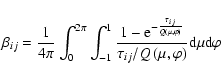
The Sobolev escape probability
.
The Sobolev escape probability
![]() is
is
and
![]() accounts for the interaction of
the continuum radiation with the transition at a given point:
accounts for the interaction of
the continuum radiation with the transition at a given point:
The optical dept of the transition is
Here nk is the kth component of the vector ![]() and rl is the
lth component of the radius vector
and rl is the
lth component of the radius vector ![]() of the point of interest (Rybicki & Hummer 1978).
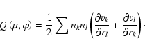
The main difference between 1D and the 3D case is the way Q is
calculated. In our code we calculate Q using all three components
of the point of interest (Rybicki & Hummer 1978).
The main difference between 1D and the 3D case is the way Q is
calculated. In our code we calculate Q using all three components
![]() of the
velocity field and their nine derivatives.
of the
velocity field and their nine derivatives.
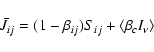
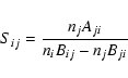
The source function Sij of the transition
![]() can be written as
can be written as
where Aji, Bij are the Einstein coefficients. Substituting Eq. (26), we
can write the bound-bound radiation rates as
when
![]() ,
,
![]() the hence the net rate
the hence the net rate
![]() assuring detailed balance in
the lines.
assuring detailed balance in
the lines.
The idea of the Sobolev approximation is to substitute the solution of the
ERT into the rate equation. This is the same idea as in the ALO method. So, one can
look at the Sobolev approximation as a ALO with
![]() .
.
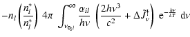
The electron thermal balance due to free-free transitions is
and the contribution of the collisional transitions is
Following the idea described in Sect. 3.1, we substitute the radiation field from (22) in (35) and (36) (see Appendix A for details). The final equation is again a function only of the unknown level populations and the temperature.
Substituting (25), (35), (36) and (37) in (17)
and (18) at each point of the wind
we obtain a system of Nl+1 equations for the Nl unknown level populations
and the unknown temperature. The system is nonlinear on the level populations due to
the products nk ni, nk nl in Eqs. (25), (35) and (36). Following
Rybicki & Hummer (1991) and de Koter et al. (1993) we remove the
nonlinearity by preconditioning. We assume that the level populations and the opacity
![]() do not vary rapidly from iteration to iteration. The
quantities in the square bracket in (25), (36) and the
opacity
do not vary rapidly from iteration to iteration. The
quantities in the square bracket in (25), (36) and the
opacity
![]() can be evaluated using the populations from the previous iteration. The resulting system
becomes linear in the level populations but it is still nonlinear in the temperature.
Unfortunately, the nonlinearity of the temperature is mainly in the form
can be evaluated using the populations from the previous iteration. The resulting system
becomes linear in the level populations but it is still nonlinear in the temperature.
Unfortunately, the nonlinearity of the temperature is mainly in the form
![]() and it is not as easy to precondition as the level populations. So we linearize the
preconditioned system in the temperature. As a result, we obtain the system
and it is not as easy to precondition as the level populations. So we linearize the
preconditioned system in the temperature. As a result, we obtain the system
To facilitate the solution, different starting models can be used, and different techniques can be used to assist in the convergence. For the starting solution we can use a previously converged model, or use the results from a 1D CMFGEN (Hillier & Miller 1998) model. Since we use preconditioning, and not linearization, it not necessary for the starting solution to be "close'' to the final solution. Thus we can even start the model using a LTE initial guess which adds just a few iterations to the model.
To facilitate convergence we initially hold the temperature constant, until the changes of level populations are reduced below some given value - usually 100%. The temperature corrections are continued until they are reduced below some specified level, usually 1%. The code then continues to iterate on the populations until the changes are reduced below some specified limit.
Ng acceleration on the level populations is started when the changes drop below some given level, usually 20-30%. Starting the acceleration earlier leads to poorer convergence, a feature noted previously by Hillier (1990) and Rybicki & Hummer (1991). Ng acceleration of the radiation field, with strong electron scattering, is applied all the time if more than 25 iterations are needed.
In some cases the convergence rate is reduced due to stabilization
or an oscillation in the corrections of a single level at one or two depth points.
Figure 2 shows the convergence
of a 1D model (Model 1, see Sect. 4.3)
compared to the same model calculated with CMFGEN. No acceleration
was applied. After the first 25 iterations, the only level whose population is
changing is He I 1s 2p 1P![]() at a single depth. During the remaining
iterations changes in this level governs the rate of convergence. This behavior
is often encountered in other models, and is also seen in some CMFGEN models
(particularly those using a diagonal operator and/or models in which not all
levels are treated in the linearization). We are working on an
algorithm which detects and avoids these kinds of problems. Our implementation of
the preconditioning converges somewhat
slower than the diagonal linearization scheme, but the difference is not
significant and cannot be considered to be a major disadvantage.
at a single depth. During the remaining
iterations changes in this level governs the rate of convergence. This behavior
is often encountered in other models, and is also seen in some CMFGEN models
(particularly those using a diagonal operator and/or models in which not all
levels are treated in the linearization). We are working on an
algorithm which detects and avoids these kinds of problems. Our implementation of
the preconditioning converges somewhat
slower than the diagonal linearization scheme, but the difference is not
significant and cannot be considered to be a major disadvantage.
![\begin{figure}
\par {\includegraphics[width=8.1cm,clip]{4666fig2.ps} }
\end{figure}](/articles/aa/full/2006/41/aa4666-05/img159.gif) |
Figure 2:
Convergence rate of Model 1 compared to the same model calculated
with CMFGEN. The two codes were run from the same initial guess. In CMFGEN a diagonal linearization scheme was used.
After iteration 25 of Model 1, the maximal relative correction
to the level populations is determined by the He I 1s 2p 1P |
| Open with DEXTER | |
In this section we present four types of tests. First we tested the performance of the short characteristics method and the ALO in one and two dimensions using the tough case of gray opacity and pure scattering. Then a complete 1D non-LTE model was run and the results were compared with the model, using the same parameters, computed by CMFGEN (Hillier & Miller 1998). Finally, we ran a full 2D model to test the performance of the code in 2D. We also use this model to discuss the effects of the deviation from the spherical symmetry. The parameters of the non-LTE models presented below are specified as described in Table 1. The models with gray opacity are described in the text.
Table 1: Parameters of the test models.
Before we could advance to the solution of the SEE we first
performed tests to check the formal solver and the construction and performance of the ALO.
We constructed a spherically symmetric envelope with pure gray scattering opacity
![]() and no thermal emission (
and no thermal emission (
![]() ,
and thus
J=S, which is equivalent to solving the radiative transfer problem for a gray opacity
source under the assumption of radiative equilibrium).
The constant C is chosen so the total radial optical depth
,
and thus
J=S, which is equivalent to solving the radiative transfer problem for a gray opacity
source under the assumption of radiative equilibrium).
The constant C is chosen so the total radial optical depth
![]() is equal to a given value
is equal to a given value
![]() and we set the total flux H to a fixed value. The solution is started
with
and we set the total flux H to a fixed value. The solution is started
with
![]() and the code runs until the fractional corrections to the
source function become less than
and the code runs until the fractional corrections to the
source function become less than ![]() .
We ran the same test using the long characteristic code
(Hillier 1996) and also compared the result with the semi analytical formula derived by
Hummer & Rybicki (1971). Figure 3 shows this comparison for
.
We ran the same test using the long characteristic code
(Hillier 1996) and also compared the result with the semi analytical formula derived by
Hummer & Rybicki (1971). Figure 3 shows this comparison for
![]() and H=1.0 for models with a different number of radial grid points. The units of the flux H are arbitrary
because the source function and the radiation field are simply proportional to this value.
In all cases, the J as a function of r is close to the other solutions. The higher number
of grid points leads to shorter characteristics. Consequently,
the optical depth along them is calculated
with better precision, the angle integration is more accurate, and the
parabolic approximation of the source function S is better. As a result we obtain a more
accurate solution as shown in Fig. 3.
and H=1.0 for models with a different number of radial grid points. The units of the flux H are arbitrary
because the source function and the radiation field are simply proportional to this value.
In all cases, the J as a function of r is close to the other solutions. The higher number
of grid points leads to shorter characteristics. Consequently,
the optical depth along them is calculated
with better precision, the angle integration is more accurate, and the
parabolic approximation of the source function S is better. As a result we obtain a more
accurate solution as shown in Fig. 3.
![\begin{figure}
\par {\includegraphics[width=7.5cm,clip]{4666fig3.ps} }
\end{figure}](/articles/aa/full/2006/41/aa4666-05/img182.gif) |
Figure 3:
Comparison between the average intensity in
a spherically symmetric wind with gray pure scattering opacity
|
| Open with DEXTER | |
Another indicator of the performance of the code is the conservation of the total flux. In a spherically symmetric atmosphere in radiative equilibrium, the quantity r2 H(r), where H(r) is the total flux at radius r, is constant. In Fig. 4, the quantity r2 H(r) is compared to its exact value H0 R*2 for models with different numbers of points in the grid. As for the average intensity, the error in the flux is reduced when the number of points in the grid is increased, which again reflects the improvement of the approximations used to calculate the radiation field.
We conclude that our implementation of the short characteristic method performs well in spherical symmetry and we move to 2D test cases.
![\begin{figure}
\par {\includegraphics[width=7.4cm,clip]{4666fig4.ps} }\end{figure}](/articles/aa/full/2006/41/aa4666-05/img183.gif) |
Figure 4: Conservation of the flux for spherical models with a different number of radial points. Solid line - 100 depth points, dashed line - 200 points, dash-dotted line - 300 points. The ordinate is the difference between the calculated and the exact flux multiplied by r2. As expected, the difference between the calculated and exact fluxes decreases with increasing numbers of points. |
| Open with DEXTER | |
The density structure of a spherically symmetric wind is defined by its mass-loss rate and the velocity field by means of the equation of continuity.
But if the wind deviates from the symmetry, its
density structure is not so simply obtained. In this paper we concentrate on a method to
model axisymmetric winds, but do not discuss the origin of the asymmetry. We assume
the wind to have a simple sine variation of the mass-loss rate
![]() with the polar distance
with the polar distance ![]() .
.
As in the 1D case, we first compare the short characteristics solver to another
short characteristics code, which was extensively tested (Busche & Hillier 2000).
The same simple pure scattering opacity with r-3 is used but with angular dependence
of the mass-loss rate from Eq. (39) with
![]() and concentration
parameter
and concentration
parameter
![]() .
The left panel of Fig. 5 shows the average intensity
calculated with the present short characteristics code divided by the J of a spherically
symmetric wind with the same opacity as on the equator.
The right panel shows the difference between the average intensity calculated
with the two short characteristics codes.
As it is seen the two codes give the same result within a few percent which,
as above, we attribute mainly to the calculation of the optical depth and the
interpolation techniques which are different in the two codes.
.
The left panel of Fig. 5 shows the average intensity
calculated with the present short characteristics code divided by the J of a spherically
symmetric wind with the same opacity as on the equator.
The right panel shows the difference between the average intensity calculated
with the two short characteristics codes.
As it is seen the two codes give the same result within a few percent which,
as above, we attribute mainly to the calculation of the optical depth and the
interpolation techniques which are different in the two codes.
![\begin{figure}
\par {\includegraphics[width=17.3cm,clip]{4666fig5.eps} }\end{figure}](/articles/aa/full/2006/41/aa4666-05/img190.gif) |
Figure 5:
Left: the ratio of the average intensity in a wind with angular
dependence of the opacity with contrast 2 and the spherically symmetric wind
with the radial distribution of the opacity as on the equator.
The pole is at |
| Open with DEXTER | |
The models discussed here have the polar wind optically thinner than the equatorial wind.
As a result, the radial component of the flux at the pole is increased with respect to the spherical
wind and the equatorial flux is reduced (Fig. 6, left). As the spherical
symmetry is broken, the ![]() component of the flux (tangential flux) is not zero.
The right panels of Fig. 6 show the variation of this
component in the wind. The behavior of the tangential flux depends not only on the contrast
between the polar and equatorial densities, but also on the actual density distribution. Right panels of
Fig. 6 show this component of the flux for two models. They have the same mass-loss rate
contrast
component of the flux (tangential flux) is not zero.
The right panels of Fig. 6 show the variation of this
component in the wind. The behavior of the tangential flux depends not only on the contrast
between the polar and equatorial densities, but also on the actual density distribution. Right panels of
Fig. 6 show this component of the flux for two models. They have the same mass-loss rate
contrast
![]() but a different concentration of the material towards the equator
(see Eq. (39) below). The iso surfaces
(for
but a different concentration of the material towards the equator
(see Eq. (39) below). The iso surfaces
(for ![]() )
of the two models are shown at the upper right corner of the right panels of Fig. 6.
As it is seen, the more toroidal star (Fig. 6, upper panels)
has tangential flux from the pole toward the equator (positive flux) at all radial distances and polar angles.
The more disk-like star (Fig. 6, lower panels) has flux which changes its direction
at different points in the wind. In general, one can attribute a force due to the radiation
pressure for each component of the flux. The presence of
)
of the two models are shown at the upper right corner of the right panels of Fig. 6.
As it is seen, the more toroidal star (Fig. 6, upper panels)
has tangential flux from the pole toward the equator (positive flux) at all radial distances and polar angles.
The more disk-like star (Fig. 6, lower panels) has flux which changes its direction
at different points in the wind. In general, one can attribute a force due to the radiation
pressure for each component of the flux. The presence of ![]() ,
which changes for different
distributions of the material, might affect the hydrodynamics of the wind.
,
which changes for different
distributions of the material, might affect the hydrodynamics of the wind.
![\begin{figure}
\par {\includegraphics[width=8.5cm,clip]{4666fig6.eps} }
\end{figure}](/articles/aa/full/2006/41/aa4666-05/img193.gif) |
Figure 6:
Left: radial flux normalized to the same value for spherical wind. Right: tangential flux.
The two models have
the same contrast
|
| Open with DEXTER | |
Once we tested the solver of the radiation transport equation and the construction of the
![]() we were able to test the entire code.
As above we first calculated 1D models and compared the results with a model with the same
parameters but calculated with CMFGEN. The test was
performed in two steps. First we checked the solution of the statistical equilibrium equation with
a fixed temperature and then we checked the temperature correction procedure.
we were able to test the entire code.
As above we first calculated 1D models and compared the results with a model with the same
parameters but calculated with CMFGEN. The test was
performed in two steps. First we checked the solution of the statistical equilibrium equation with
a fixed temperature and then we checked the temperature correction procedure.
For the first test we chose the velocity structure as described in Hillier & Miller (1998) with parameters described in Table 1, Model 0 and the number of radial points Nr=60 . The solution was started with the temperature distribution of the converged CMFGEN model with the same parameters, but the starting level population and electron density was set to LTE. We calculated the same model with CMFGEN setting the code to use the Sobolev approximation and atoms with the same number of levels. The departure coefficients of the first five H I levels are shown in Fig. 7 together with the results obtained with CMFGEN. The two codes give results which differ by less than 3%. Again, we checked the behavior of the difference by increasing the number of grid points. The departure coefficient for the first level of H I for the model with Nr=120 radial points is shown in Fig. 7 with diamonds. As one might expect, the difference between the two models decreases with increasing Nr.
![\begin{figure}
\par {\includegraphics[width=6.9cm,clip]{4666fig7.ps} }\end{figure}](/articles/aa/full/2006/41/aa4666-05/img194.gif) |
Figure 7: Comparison between departure coefficients of the first five hydrogen levels for Model 0 (Table 1) calculated with CMFGEN (dashed lines) and the new code (solid lines). The curves for different levels are marked. The diamonds show the departure coefficient for the first H I level for a model with the same parameters but with twice as many radial points. |
| Open with DEXTER | |
The same model, but with added carbon levels (Model 1 in Table 1), was used to test the temperature correction procedure (Fig. 8). As in the case of the departure coefficients, the temperature distribution obtained with the new code was in good agreement with the temperature obtained with CMFGEN. As expected the emitted spectrum calculated with the new code's level populations also agrees well with the one calculated with CMFGEN. Figure 9 shows some of the lines of HI, HeI, HeII and CIV usually used for wind diagnostics. The spectra calculated by the two codes differ by less than 1%. For the test we switched off the dielectronic recombination and level dissolution which are treated in CMFGEN but are not yet implemented into the new code.
![\begin{figure}
\par {\includegraphics[width=7.8cm,clip]{4666fig8.ps} }\end{figure}](/articles/aa/full/2006/41/aa4666-05/img195.gif) |
Figure 8: Comparison between temperature distribution of Model 1 (Table 1) calculated with CMFGEN (dashed line) and the new code (solid line). The maximal difference is less than 3%. |
| Open with DEXTER | |
| |
Figure 9: Comparison between the emitted spectrum of Model 1 (Table 1) calculated with CMFGEN (thick gray line) and the new code (thin black line). The maximal difference is less than 1%. |
| Open with DEXTER | |
We introduced axial symmetry into the models by two means.
First we modified the mass-loss rate at each polar distance as described in
4.2, Eq. (39). In the same way we assume an axisymmetric terminal
velocity ![]() but we keep the flow radial, with the radial velocity obeying the
standard velocity law:
but we keep the flow radial, with the radial velocity obeying the
standard velocity law:
 |
(44) |
![\begin{figure}
\par {\includegraphics[width=6.9cm,clip]{4666fig9.ps} }\end{figure}](/articles/aa/full/2006/41/aa4666-05/img209.gif) |
Figure 10: Temperature structure of 2D wind. The rapid rise of the temperature toward the pole is caused by the ionization of C IV which reduces the cooling. |
| Open with DEXTER | |
| |
Figure 11: Helium ionization. Left: He II; Right He III. |
| Open with DEXTER | |
The helium ionization balance shows a similar pattern. As often occurs in an O star's wind, He III recombines to He II in the region where the velocity increases to supersonic values. Subsequently, the ionization increases and the wind is maintained completely ionized. The more pronounced dip in the helium ionization creates a more pronounced rise in the temperature. Again, a strong ionization front in the tangential direction is formed in the outer part of the wind (Fig. 11). As we said above, we do not attempt to model a real wind in this paper. However even these simple calculations show that behavior of the ionization points to a possible correlation between the line strength, the line profile and the ionization stage, which could be used as a diagnostic tool.
| |
Figure 12:
Carbon ionization. Left: C IV, Right: C V.
The increase in the ionization of C IV near the pole ( |
| Open with DEXTER | |
In this paper we have described a code we have developed to model non-spherically symmetric stellar winds. The code is based on a short characteristics solver for the radiation transport, preconditioning of the equations of statistical equilibrium combined with linearization of the electron thermal balance equation. Extensive testing of the code has been undertaken in order to verify its correctness. Importantly, the tests show that the short characteristics method, combined with ALO, preconditioning of the statistical equilibrium equations and the temperature correction based on the electron thermal balance, can model 2D winds.
The main limitation of the current version of the code is the Sobolev approximation which we will improve with the implementation of the new solver described in Zsargó et al. (2006). However we have designed the code with flexibility in mind, and it is relatively straightforward to insert alternative radiation field solvers. As expected, the increase in the number of dimensions increases the time per iteration. Fortunately, the short characteristics method allows for relatively easy parallelization which will also be implemented in the next version.
Even a simple model of an axisymmetric wind, as presented here, shows important differences in its temperature and ionization structure compared with a spherically symmetric wind. Such differences are expected, and are seen in other calculations (e.g., Kraus & Lamers 2003). The differences will cause changes in the emitted spectrum which in turn will provide observable diagnostics for the deviation from symmetry. Computations with the newly developed code will also be important for investigating the importance of the influence of the tangential flux on the hydrodynamics of stellar winds. Calculations show, for example, that the tangential flux can suppress the formation of wind compressed disks (Owocki et al. 1996).
The code, and implemented methods, are very flexible and allow the application of the code to many different objects with complex velocity fields such as accretion disks, rotating winds, interacting winds in binary systems and asymmetric outbursts in novae or supernovae.
Acknowledgements
This work was partially supported by Mexico CONACyT grants 40864-F and 42809 (L.G.). Support from NSF grants AST-9987390 and AST-0507328 is gratefully acknowledged.
We have previously shown that the net rate in a bound-free transition
can be written as
Ak =  |
(A.5) |
Bm =  |
(A.6) |
ak =  |
(A.7) |
| bm = |
(A.8) |
Having in mind that
 |
(A.15) |
 |
(A.16) |
 |
(A.17) |
Finally we deduce the heating-cooling balances. The balance between heating and cooling by bound-free transitions is more
laborious. But, if we define
![]() as in (35), the balance
as in (35), the balance
![]() becomes
becomes
The same idea gives us the collisional thermal balance
![]() and its derivative.
and its derivative.
| = |  |
||
 |
= |  |
(A.25) |
The last term in (18) is the free-free transitions temperature balance, given by
 |
(A.26) |
![$\displaystyle \frac{\partial }{\partial T}\Delta Q_{\rm ff}^m =
N_{\rm e} n_m 4...
...nu(T))
-\chi_{\rm ff}^m \frac{\partial }{\partial T}B_\nu(T) \right] {\rm d}\nu$](/articles/aa/full/2006/41/aa4666-05/img264.gif) |
(A.27) |
| |
= |  |
(A.28) |
| = | (A.29) |
These equations define all necessary members of the system (38), and its solution give the unknown
level populations ni and the correction to the temperature ![]() .
.

![$\displaystyle + \sum_k n_k ~ 4\pi ~ \int_{\nu_{0_{il}}}^\infty \frac{\alpha_{il...
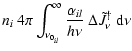
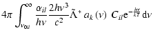
...left(\frac{n_i^*}{n_l^*}\right)~ {\rm e}^{-\frac{h\nu}{kT}}\right] ~ {\rm d}\nu$](/articles/aa/full/2006/41/aa4666-05/img117.gif)
![$\displaystyle + \sum_m n_m ~ 4\pi ~ \int_{\nu_{0_{il}}}^\infty \frac{\alpha_{il...
...ft(\frac{n_i^*}{n_l^*}\right)~ {\rm e}^{-\frac{h\nu}{kT}}\right] ~ {\rm d}\nu .$](/articles/aa/full/2006/41/aa4666-05/img118.gif)


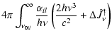
![$\displaystyle \Delta Q_{\rm ff} = 4 \pi N_{\rm e} \sum_m n_m \int_0^\infty
\alp...
...kT}}\right)- \frac{2 h \nu^3}{c^2}{\rm e}^{-\frac{h\nu}{kT}} \right]{\rm d}\nu,$](/articles/aa/full/2006/41/aa4666-05/img151.gif)
![$\displaystyle +\left[-\sum_{j<i} \frac{\partial }{\partial T}\Gamma_{ji} + \sum...
...}\Xi_{ji} + \sum_{j>i} \frac{\partial }{\partial T}\Xi_{ij}\right] \Delta T = 0$](/articles/aa/full/2006/41/aa4666-05/img155.gif)
![$\displaystyle +\left[\frac{\partial }{\partial T}\Delta Q_{\rm bf} + \frac{\par...
...{\rm ff} + \frac{\partial }{\partial T}\Delta Q_{\rm coll}\right] \Delta T = 0.$](/articles/aa/full/2006/41/aa4666-05/img157.gif)
![\begin{displaymath}\dot M(\beta) = {\dot M \over M_{\rm contr}} \left( 1 + \left[M_{\rm contr} -1 \right]\sin^{\alpha_1}\beta\right)
\end{displaymath}](/articles/aa/full/2006/41/aa4666-05/img185.gif)
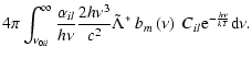
![$\displaystyle + \sum_m n_m ~ 4\pi ~ \int_{\nu_{0_{il}}}^\infty \frac{\alpha_{il...
...left(\frac{n_i^*}{n_l^*}\right)~ {\rm e}^{-\frac{h\nu}{kT}}\right] ~ {\rm d}\nu$](/articles/aa/full/2006/41/aa4666-05/img213.gif)
![$\displaystyle \left[n_i-n_l\left(\frac{n_i^*}{n_l^*}\right){\rm e}^{-\frac{h\nu}{kT}}\right].$](/articles/aa/full/2006/41/aa4666-05/img216.gif)
![$\displaystyle \Gamma_{il}^{2}+\Gamma_{il}^{3l}+\Gamma_{il}^{4l} =
-4\pi \int_{\...
...t] + \Delta \tilde{J}^\dagger_\nu\right)
{\rm e}^{-\frac{h\nu}{kT}} {\rm d}\nu.$](/articles/aa/full/2006/41/aa4666-05/img234.gif)
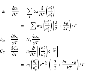
![$\displaystyle \times \left[-\left(\frac{n_i^*}{n_l^*}\right) \left(\frac{3}{2}+...
...{il}}{kT}\right)/T+\frac{h\nu}{kT^2}\right]{\rm e}^{-\frac{h\nu}{kT}}{\rm d}\nu$](/articles/aa/full/2006/41/aa4666-05/img240.gif)
![$\displaystyle \times \left[\dot a_k C_{il}+a_k \dot C_{il}+a_k C_{il} \frac{h\nu}{kT^2}\right]{\rm e}^{-\frac{h\nu}{kT}}{\rm d}\nu$](/articles/aa/full/2006/41/aa4666-05/img243.gif)
![$\displaystyle \times \left[\dot b_m C_{il}+b_m \dot C_{il}+b_m C_{il} \frac{h\nu}{kT^2}\right]{\rm e}^{-\frac{h\nu}{kT}}{\rm d}\nu$](/articles/aa/full/2006/41/aa4666-05/img245.gif)
![$\displaystyle \frac{\partial}{\partial T} \Xi_{ij} =
n_i N_{\rm e} q_{ij}\left[...
... \ln{q_{ij}}}{\partial T}\right)\frac{n_j}{n_i}
\frac{n_i^*}{n_l^*}\right]\cdot$](/articles/aa/full/2006/41/aa4666-05/img252.gif)