A&A 457, 707-715 (2006)
DOI: 10.1051/0004-6361:20065524
G. R. Donnelly - A. J. Díaz - B. Roberts
Mathematical Institute, University of St Andrews, St Andrews KY16 9SS, Scotland, UK
Received 28 April 2006 / Accepted 3 July 2006
Abstract
Aims. We investigate the influence of longitudinal structuring of the surrounding corona on the modes of oscillation of a coronal magnetic flux tube.
Methods. A partial differential equation is derived for the total pressure perturbation of the fast modes and it is solved analytically in terms of Bessel functions, obtaining a dispersion relation.
Results. The introduction of coronal structuring changes the cutoff frequency, enhancing coronal leakage, so even the fundamental kink mode may become leaky. Structure also modifies the loop's oscillatory frequencies and may result in higher harmonics being trapped.
Conclusions. Depending on the structuring, two competing effects take place: environmental structuring enhances leakage, while loop structuring helps confine the modes. This has important consequences for coronal seismology, leading to the absence of trapped modes for certain parameters and shifts in frequencies.
Key words: Sun: oscillations - Sun: magnetic fields - Sun: corona
An important feature of the solar corona is the wide variety of structures which occur as a result of the Sun's complex magnetic field. Many of these structures share the feature that they have a density enhancement (high plasma density compared with the surrounding plasma), allowing them to act as an MHD wave guide. They may also have temperature or magnetic field enhancements or depletions, but in the low-![]() corona it is density (and through this the Alfvén speed) that plays the major role.
corona it is density (and through this the Alfvén speed) that plays the major role.
The excellent observational ability of spacecrafts such as TRACE and SOHO has provided us with an array of detections of both standing (Aschwanden et al. 2002; Ofman & Wang 2002; Nakariakov et al. 1999; Aschwanden et al. 1999; Wang et al. 2002c,2003,2002b,a; Schrijver et al. 2002; Schrijver & Brown 2000) and propagating (De Moortel et al. 2002b; Williams et al. 2001; Robbrecht et al. 2000; De Moortel et al. 2002c; Williams et al. 2002; Berghmans & Clette 1999; De Moortel et al. 2000) waves occurring in coronal loops. Despite these capabilities it is still difficult to make direct observations of fundamental quantities such as the magnetic field strength. However, the technique of coronal seismology (McEwan et al. 2006; Nakariakov et al. 1999; Andries et al. 2005a; De Moortel et al. 2002a; Roberts et al. 1984; Andries et al. 2005b; Roberts 1986; Nakariakov & Ofman 2001) allows information carried by MHD waves to be extracted from observations of oscillatory events and the results interpreted using theoretical models.
There have been several theoretical models of coronal loops. The first models considered only the simplest aspects of magnetic structuring, using a Cartesian slab (e.g. Roberts 1981; Edwin & Roberts 1982) or a cylindrical tube (e.g. Edwin & Roberts 1983; Spruit 1982). In cylindrical models the coronal loop is represented by an infinitely long and straight uniform magnetic flux tube. The loop has a plasma density enhancement compared with its environment, and the magnetic field is directed along the loop. This configuration produces a rich array of wave behaviour and is widely used in coronal seismology. From this model several features may be added, such as the presence of magnetic twist (Sakai et al. 2000; Bennett et al. 1999), or field-aligned flows (Nakariakov & Roberts 1995; Terra-Homem et al. 2003; Somasundaram et al. 1999), the role of line-tying effects (Díaz et al. 2004), longitudinal stratification (Roberts 2006; Mendoza-Briceño et al. 2004; Andries et al. 2005b; James 2003; Nakariakov & Ofman 2001; Nakariakov et al. 2000), curvature (Verwichte et al. 2006; Díaz 2006; Smith et al. 1997; Selwa et al. 2005; Van Doorsselaere et al. 2004; Díaz et al. 2006b; Brady & Arber 2005), coronal leakage (Cally 2003; Díaz et al. 2004; Cally 1986; Brady & Arber 2005), magnetic shells (Mikhalyaev & Solov'ev 2005; Erdelyi & Carter 2006), loops of elliptical cross-section (Ruderman 2003) or multithreaded loops (Oliver et al. 2006; Gruszecki et al. 2006). Extensive reviews can be found in (Nakariakov & Verwichte 2005; Aschwanden 2004).
Despite extensive work there are still many aspects of coronal loop
oscillations and coronal seismology to be explored. Here we consider the role
of footpoint structuring in the loop and the coronal environment. We consider a
uniform line-tied loop with longitudinal structuring in the loop's environment
by incorporating a dense chromospheric layer. The chromospheric layer modifies
the properties of the modes (Díaz et al. 2004), but its
inclusion in the surrounding medium has other consequences which are explored
in this paper. In an unbounded homogeneous loop of radius a, the
fundamental kink mode propagates as a trapped mode for all wavenumbers k,
with a phase speed equal to the kink speed ck in the thin tube (![]() )
limit (Edwin & Roberts 1983; Spruit 1982).
However, for a suitable depth of chromospheric layer, we find
that the kink mode no longer propagates as a trapped mode. Also, in the case
where it is trapped in the thin tube limit, it now propagates with a kink speed
that is modified by the presence of the chromospheric layer.
)
limit (Edwin & Roberts 1983; Spruit 1982).
However, for a suitable depth of chromospheric layer, we find
that the kink mode no longer propagates as a trapped mode. Also, in the case
where it is trapped in the thin tube limit, it now propagates with a kink speed
that is modified by the presence of the chromospheric layer.
Many results of coronal seismology, such as the deduction of the coronal magnetic field strength from the TRACE loop oscillations (Nakariakov & Ofman 2001), use the fact that the fundamental kink mode is trapped in the thin tube limit and is propagating at the kink speed. The result that the fundamental kink mode may not be trapped in the thin tube limit may thus have important implications for coronal seismology.
We consider a spatially structured static equilibrium of a cylindrically
symmetric line-tied coronal loop or magnetic flux tube (lying parallel to the
z axis) of length 2 L and radius a. The magnetic field
![]() is assumed to be uniform throughout the medium
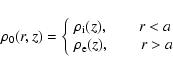
and aligned with the loop. The equilibrium density
is assumed to be uniform throughout the medium
and aligned with the loop. The equilibrium density
![]() is structured
in both the radial and longitudinal directions. Gravitational effects are
ignored.
is structured
in both the radial and longitudinal directions. Gravitational effects are
ignored.
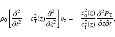
Small amplitude oscillations about this equilibrium are introduced. The ideal adiabatic MHD equations (neglecting gravitational effects) reduce to the following system of coupled partial differential equations (see, for example, Díaz et al. 2002; Roberts 1991)
The low ![]() or cold plasma approximation (
or cold plasma approximation (![]() )
is now taken, in which
we neglect the effect of plasma pressure; this is a good approximation in the
corona where the plasma beta is small. Consequently, the slow mode is removed
from the system, since Eq. (3) becomes decoupled and gives
vz=0. Some care should be taken in making this approximation to other
regions of the solar atmosphere, such as the chromosphere or photosphere, as
pressure effects and gravitational stratification play a greater role in these
layers (see Roberts 2004, for a recent discussion). The implication of the
)
is now taken, in which
we neglect the effect of plasma pressure; this is a good approximation in the
corona where the plasma beta is small. Consequently, the slow mode is removed
from the system, since Eq. (3) becomes decoupled and gives
vz=0. Some care should be taken in making this approximation to other
regions of the solar atmosphere, such as the chromosphere or photosphere, as
pressure effects and gravitational stratification play a greater role in these
layers (see Roberts 2004, for a recent discussion). The implication of the
![]() limit on the speeds of the system are that
limit on the speeds of the system are that
![]() ,
,
![]() and
and
![]() so
acoustic aspects are lost and the fast modes are decoupled from the Alfvén waves;
hence the zero-
so
acoustic aspects are lost and the fast modes are decoupled from the Alfvén waves;
hence the zero-![]() assumption allows a study of fast modes to be
undertaken.
assumption allows a study of fast modes to be
undertaken.
We allow for a general longitudinal and transverse structuring in the form of step functions, the equilibrium plasma density profile taking the form
We consider trapped modes for which there is no propagation of energy towards or
away from the loop. This is achieved by imposing
![]() and
and
![]() as
as
![]() .
The loop is line-tied with the footpoints fixed in the dense photosphere, where it is expected that coronal perturbations carry such small energy that they are incapable of perturbing the dense photospheric plasma; this leads to the line-tying boundary condition
.
The loop is line-tied with the footpoints fixed in the dense photosphere, where it is expected that coronal perturbations carry such small energy that they are incapable of perturbing the dense photospheric plasma; this leads to the line-tying boundary condition
![]() .
In this model we have interfaces over which the equilibrium plasma properties jump discontinuously so we must know how the perturbations behave across such surfaces. There are two types of interface: those parallel to the applied equilibrium magnetic field and those which are not parallel to the equilibrium magnetic field. In the case where the interface is parallel to the equilibrium field, the boundary conditions are (Goedbloed 1983; Díaz et al. 2001; Díaz 2004)
.
In this model we have interfaces over which the equilibrium plasma properties jump discontinuously so we must know how the perturbations behave across such surfaces. There are two types of interface: those parallel to the applied equilibrium magnetic field and those which are not parallel to the equilibrium magnetic field. In the case where the interface is parallel to the equilibrium field, the boundary conditions are (Goedbloed 1983; Díaz et al. 2001; Díaz 2004)
For interfaces which are not parallel to the equilibrium magnetic field, the boundary conditions are
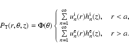
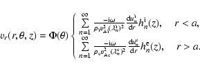
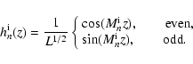
We study oscillatory solutions to Eq. (5) in cylindrical
coordinates. Following Díaz et al. (2002), we assume a solution which is separable
in space and Fourier analysing in time, writing
![]() in the form
in the form
Solving Eq. (10) for ![]() gives
gives
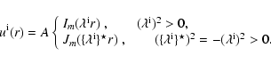
Equation (9) for u(r) inside the loop has the form of a Bessel (or
modified Bessel) equation of order m for
![]() (or
(or
![]() ); we write
); we write
In the environment of the tube the equation for u(r) takes the form of a
modified Bessel equation; since we consider trapped modes, it is required
that all perturbations decline to zero as
![]() ,
with the
implication that
,
with the
implication that
![]() and then
and then
![\begin{figure}
\par\includegraphics[width=5.6cm,clip]{5524f1.eps}
\end{figure}](/articles/aa/full/2006/38/aa5524-06/img84.gif) |
Figure 1:
A sketch of the equilibrium configuration showing a slice (in r and
z) of a cylindrically symmetric uniform coronal loop, of length 2L and
radius a. The plasma density in the tube interior is
|
| Open with DEXTER | |
In order to investigate the effect of chromospheric layers on the oscillations
of a coronal loop we consider first the special case of an entirely uniform
loop surrounded by a coronal environment with chromospheric layers. This allows a
more straightforward discussion of the new effects. Later, we return to the
more realistic model in which the chromospheric layers occur both inside and
outside the loop. Consider, then, the equilibrium configuration of
Fig. 1, but here assuming an entirely uniform loop profile,
of density
![]() .
The chromospheric inhomogeneity is then
confined entirely to the loop's environment, so that for r > a the
density profile is
.
The chromospheric inhomogeneity is then
confined entirely to the loop's environment, so that for r > a the
density profile is
![\begin{displaymath}\int_{-L}^L\left[ h_n^{\rm i}(z)\right]^2 {\rm d}z=\int_{-L}^L\left[ h_n^{\rm e}(z)\right]^2 {\rm d}z=1 .
\end{displaymath}](/articles/aa/full/2006/38/aa5524-06/img91.gif) |
(27) |
The line tying condition
![]() is automatically satisfied by our
choice of solution (26) in the loop environment, but
is automatically satisfied by our
choice of solution (26) in the loop environment, but
![]() is restricted to be
is restricted to be
The final coefficient we require, in order to evaluate the determinant of the
system of Eqs. (23) and obtain our dispersion relation, are the
values of Hnm. For the even modes, the coefficients Hnm are evaluated using
Eq. (18), giving
There is a similar form for the Hnm coefficient in the case of the odd modes.
![\begin{figure}
\par\mbox{\subfigure[]{\includegraphics[width=6cm,clip]{5524f2a.e...
...{4mm}
\subfigure[]{\includegraphics[width=6cm,clip]{5524f2b.ps} } }
\end{figure}](/articles/aa/full/2006/38/aa5524-06/img121.gif) |
Figure 2:
a) Dispersion diagram for
|
| Open with DEXTER | |
We first study the dispersive nature of the modes as the ratio a/L of
the loop radius to the loop half-length varies. Figure 2a shows
the dispersion diagram for the even modes, for appropriate coronal parameters.
The dispersion diagram displays a band of dispersive fast modes, similar in
behaviour to those of Edwin & Roberts (1983). There is only one mode propagating in the
thin tube limit ![]() ,
which is the fundamental kink mode with
frequency
,
which is the fundamental kink mode with
frequency
![]() .
This differs from the frequency of
the fundamental kink mode in a homogeneous environment, which gives
.
This differs from the frequency of
the fundamental kink mode in a homogeneous environment, which gives
![]() for these parameters. The sausage modes and the higher harmonics
of the kink modes all have cutoff frequencies, so none propagate in the thin
tube limit. Figure 2b shows the
same plot of the dispersion diagram displayed in Fig. 2a but here
with lengths normalised against the loop radius a. This plot is
useful for coronal seismology, since it relates the frequency of the mode with
the loop length, which can be deduced in many of the observations.
In accordance with
Edwin & Roberts (1983), the frequency for the fundamental kink mode is almost insensitive
to the loop radius for realistic values of L / a (
for these parameters. The sausage modes and the higher harmonics
of the kink modes all have cutoff frequencies, so none propagate in the thin
tube limit. Figure 2b shows the
same plot of the dispersion diagram displayed in Fig. 2a but here
with lengths normalised against the loop radius a. This plot is
useful for coronal seismology, since it relates the frequency of the mode with
the loop length, which can be deduced in many of the observations.
In accordance with
Edwin & Roberts (1983), the frequency for the fundamental kink mode is almost insensitive
to the loop radius for realistic values of L / a (![]() 101-104).
This is a useful property for coronal
seismology, since errors due to inaccuracy in determining the loop radius are
minimal if the mode observed is the fundamental kink mode.
101-104).
This is a useful property for coronal
seismology, since errors due to inaccuracy in determining the loop radius are
minimal if the mode observed is the fundamental kink mode.
The cutoff curve is marked by a dotted line showing the cutoff frequency
![]() ,
with
,
with
![]() in
Fig. 2. Therefore, we observe an immediate consequence of
the chromospheric layer, which causes the cutoff frequency to shift from its
value
in
Fig. 2. Therefore, we observe an immediate consequence of
the chromospheric layer, which causes the cutoff frequency to shift from its
value
![]() in
a homogeneous environment (Eq. (15)), independently of the
internal structure of the loop.
in
a homogeneous environment (Eq. (15)), independently of the
internal structure of the loop.
The parameter W/L provides a measure of the extent of the chromosphere. This
parameter leads to two limiting cases,
![]() and
and
![]() ,
in which the longitudinal structuring is eliminated and the
loop's environment becomes uniform. In both cases we expect a structure similar
to that found in Edwin & Roberts (1983). The first case,
,
in which the longitudinal structuring is eliminated and the
loop's environment becomes uniform. In both cases we expect a structure similar
to that found in Edwin & Roberts (1983). The first case,
![]() ,
consists
of a uniform loop embedded in a dense chromospheric plasma. The loop has an
enhancement in Alfvén speed over its environment and so is incapable of supporting
trapped modes of oscillation. The second case, of
,
consists
of a uniform loop embedded in a dense chromospheric plasma. The loop has an
enhancement in Alfvén speed over its environment and so is incapable of supporting
trapped modes of oscillation. The second case, of
![]() ,
consists of a loop embedded in low density coronal material. In this case the
loop has a depression in Alfvén speed compared with its environment, which is
exactly the structure Edwin & Roberts (1983) found to support trapped modes of
oscillation.
,
consists of a loop embedded in low density coronal material. In this case the
loop has a depression in Alfvén speed compared with its environment, which is
exactly the structure Edwin & Roberts (1983) found to support trapped modes of
oscillation.
It is interesting to examine the effect of letting
![]() ,
on
the system in Eq. (23). The first thing to note is that the
solutions to Eq. (9) inside and outside the loop become
identical for n=m, and hence these solutions are orthogonal; therefore,
,
on
the system in Eq. (23). The first thing to note is that the
solutions to Eq. (9) inside and outside the loop become
identical for n=m, and hence these solutions are orthogonal; therefore,
 |
(34) |
Figure 3 displays the dimensionless frequency against W / L
for a thin tube, a/ L=0.1,
so essentially plots the variation of the modified kink speed, ck, as a
function of W/L. We see that in the limit
![]() only the
fundamental kink mode is trapped; this is similar to the case in
Fig. 2.
The most striking difference between Fig. 3 and those against
a/L is that the cutoff curve exhibits a non-uniform variation, varying
from
only the
fundamental kink mode is trapped; this is similar to the case in
Fig. 2.
The most striking difference between Fig. 3 and those against
a/L is that the cutoff curve exhibits a non-uniform variation, varying
from
![]() as
as
![]() to
to
![]() as
as
![]() .
This variability in
the cutoff frequency is perhaps expected from the presence of the parameter Win Eqs. (31) and (32) and is independent of
a/L. As a result of the non-uniform cutoff curve, each mode has a
cutoff frequency and value of W / L for which the mode becomes leaky and
this is specific to that mode; this is in contrast to the uniform tube, where
all cutoff frequencies are the same.
.
This variability in
the cutoff frequency is perhaps expected from the presence of the parameter Win Eqs. (31) and (32) and is independent of
a/L. As a result of the non-uniform cutoff curve, each mode has a
cutoff frequency and value of W / L for which the mode becomes leaky and
this is specific to that mode; this is in contrast to the uniform tube, where
all cutoff frequencies are the same.
For values of a/ L larger than one there are many trapped
sausage and kink modes present for a relatively small range of chromospheric
depths (
![]() ), as would be expected from Fig. 2
for a large value of a/ L. The frequencies are almost independent of
chromospheric depth, provided they lie below the cutoff curve. However, even
the fundamental kink mode also has a cutoff frequency for small W / L. For
further details in this range see Donnelly (2006).
), as would be expected from Fig. 2
for a large value of a/ L. The frequencies are almost independent of
chromospheric depth, provided they lie below the cutoff curve. However, even
the fundamental kink mode also has a cutoff frequency for small W / L. For
further details in this range see Donnelly (2006).
![\begin{figure}
\par\includegraphics[width=7.8cm,clip]{5524f3.ps}
\end{figure}](/articles/aa/full/2006/38/aa5524-06/img136.gif) |
Figure 3:
Plot of the dimensionless frequency
|
| Open with DEXTER | |
To investigate the effect of the chromospheric layers on the nature of the
fundamental kink mode we plot in Fig. 4 a superposition of the
dispersion curves and cutoff curves on a single diagram. Three cases are
displayed:
![]() for which
for which
![]() ;
;
![]() for which
for which
![]() ;
and
;
and
![]() for which
for which
![]() .
Thus, we evolve the diagram from the case of the chromosphere being
64 times denser than the coronal region to the case of a nearly uniform
environment (low-density chromosphere). The cutoff curves evolve from one of
steep gradients to a flat curve (which would be a straight line in the case
.
Thus, we evolve the diagram from the case of the chromosphere being
64 times denser than the coronal region to the case of a nearly uniform
environment (low-density chromosphere). The cutoff curves evolve from one of
steep gradients to a flat curve (which would be a straight line in the case
![]() ,
no chromosphere). Also, the range of W /Lallowing the loop to trap the fundamental kink mode increases from the
relatively small range of
,
no chromosphere). Also, the range of W /Lallowing the loop to trap the fundamental kink mode increases from the
relatively small range of
![]() when
when
![]() to being trapped for all values of W / L in the final case,
when
to being trapped for all values of W / L in the final case,
when
![]() .
The dispersion becomes less pronounced
as the curves move towards a uniform environment model.
.
The dispersion becomes less pronounced
as the curves move towards a uniform environment model.
![\begin{figure}
\par\includegraphics[width=7.8cm,clip]{5524f4.ps}
\end{figure}](/articles/aa/full/2006/38/aa5524-06/img141.gif) |
Figure 4:
Superposition of plots of dimensionless frequency
|
| Open with DEXTER | |
Previous work has shown that in a cylindrical geometry the eigenfunctions of
such trapped modes do not penetrate deeply into the environment of the loop
(Díaz et al. 2001,2004) and so would have no strong
interaction with neighbouring structures, although as the mode propagates close
to its cutoff frequency its eigenfunctions are expected to penetrate further
into the environment. However, this is not the behaviour here. Figure 5
gives the evolution of the dimensionless total pressure perturbation at
the loop apex (z=0) as a function of radial coordinate (panel a) and at the
loop boundary (r=a) as a function of the longitudinal coordinate (panel b),
along the dispersion curve displayed in Fig. 3. There is little
difference in the penetrations of the eigenfunctions between a point close to
the cutoff frequency (Fig. 5a, solid line) and a point far from it
(Fig. 5a, dashed line). This suggests that the interaction between
neighbouring loops is weak, unless the loops are in a tightly packed group.
Figure 5b shows that the structure of the eigenfunction
evolves along the dispersion curve. At W/L=0.99,
![]() behaves much as
expected for the fundamental kink mode, having one extremum in both the radial
and longitudinal directions. However, for W/L=0.79 the eigenfunction has
developed three extrema in the longitudinal direction, although it retains the
single extrema in the radial direction.
behaves much as
expected for the fundamental kink mode, having one extremum in both the radial
and longitudinal directions. However, for W/L=0.79 the eigenfunction has
developed three extrema in the longitudinal direction, although it retains the
single extrema in the radial direction.
![\begin{figure}
\par\mbox{\subfigure[]{\includegraphics[width=6cm,clip]{5524f5a.p...
...4mm}
\subfigure[]{\includegraphics[width=6cm,clip]{5524f5b.ps} }}\end{figure}](/articles/aa/full/2006/38/aa5524-06/img142.gif) |
Figure 5:
Plots of
|
| Open with DEXTER | |
![\begin{figure}
\par\mbox{\subfigure[]{\includegraphics[width=6cm,clip]{5524f6a.p...
...e{4mm}
\subfigure[]{\includegraphics[width=6cm,clip]{5524f6b.ps} }}
\end{figure}](/articles/aa/full/2006/38/aa5524-06/img143.gif) |
Figure 6:
Plots showing
|
| Open with DEXTER | |
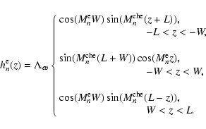
In the previous section we discussed the simplified case of a uniform loop lying within an environment structured by the presence of chromospheric layers. We now turn to the more realistic case in which chromospheric layers arise both inside and outside the loop (Fig. 1).
We consider a longitudinally structured loop of length 2L and radius
a. The structuring in the environment region is the same as discussed
previously. The loop has a uniform coronal region of extent 2W and a uniform
chromospheric region of depth (L-W) at either end of the loop. These four
regions are denoted by subscripts "e'', "che'', "i'' and "chi'', respectively. The same general procedure
is followed as previously, resulting in a solution
![]() in the region r
< a which is of the same form as
in the region r
< a which is of the same form as
![]() discussed earlier. Note that
the sign of
discussed earlier. Note that
the sign of
![]() is unrestricted as we may consider both body and
surface modes; this results in hyperbolic, rather than trigonometric,
behaviour. The solutions
is unrestricted as we may consider both body and
surface modes; this results in hyperbolic, rather than trigonometric,
behaviour. The solutions
![]() in the environment (r > a) remain
as before. The same boundary conditions are applied at each interface, with the
addition of the interface perpendicular to the magnetic field inside the loop.
We make use of the Sturm-Liouville theorem (Arfken 1985) which states that the
solutions of an eigenvalue equation such as (11) in self-adjoint
form with boundary conditions
in the environment (r > a) remain
as before. The same boundary conditions are applied at each interface, with the
addition of the interface perpendicular to the magnetic field inside the loop.
We make use of the Sturm-Liouville theorem (Arfken 1985) which states that the
solutions of an eigenvalue equation such as (11) in self-adjoint
form with boundary conditions
![]() form a complete set on the
region
form a complete set on the
region
![]() .
The Sturm-Liouville theorem guarantees that the the
eigenvalues of this equation are ordered, countable and form a complete basis.
Therefore, we may apply the Sturm-Liouville theorem to expand the external
solution
.
The Sturm-Liouville theorem guarantees that the the
eigenvalues of this equation are ordered, countable and form a complete basis.
Therefore, we may apply the Sturm-Liouville theorem to expand the external
solution
![]() in terms of the internal solutions
in terms of the internal solutions
![]() (Díaz et al. 2004).
(Díaz et al. 2004).
These steps lead to a dispersion relation taking an identical form to
Eqs. (23) from the previous case. However, the modification of
![]() due to the internal structure of the loop results in changes
to the set of
due to the internal structure of the loop results in changes
to the set of
![]() ,
which are solutions of
,
which are solutions of
There are two main cases of interest: the case where the loop footpoint is
denser than the surrounding chromosphere (resulting in the footpoint having a
depression in Alfvén speed compared with its surroundings), so
![]() ;
and the case when the loop footpoint is less dense than the
surrounding chromosphere (giving a footpoint with an enhancement in Alfvén speed
compared with its surroundings), so
;
and the case when the loop footpoint is less dense than the
surrounding chromosphere (giving a footpoint with an enhancement in Alfvén speed
compared with its surroundings), so
![]() .
If
.
If
![]() ,
we expect trapped modes to propagate in the limit
,
we expect trapped modes to propagate in the limit
![]() since the loop still has a density enhancement over its surroundings and so
may act as a waveguide. This is illustrated by
Fig. 6a, showing the dispersion diagram for
since the loop still has a density enhancement over its surroundings and so
may act as a waveguide. This is illustrated by
Fig. 6a, showing the dispersion diagram for
![]() ,
,
![]() and
and
![]() ,
with a/L
=0.1. The dispersion curve shown is the fundamental kink mode. The kink mode
now propagates as a trapped mode for all W / L. Also in
Fig. 6a we can see the cutoff frequency which varies with W /
L and is the same as in Fig. 3; as expected, the cutoff
frequency is independent of the internal structure of the loop.
,
with a/L
=0.1. The dispersion curve shown is the fundamental kink mode. The kink mode
now propagates as a trapped mode for all W / L. Also in
Fig. 6a we can see the cutoff frequency which varies with W /
L and is the same as in Fig. 3; as expected, the cutoff
frequency is independent of the internal structure of the loop.
The second case of interest is when
![]() ,
so that
the loop footpoint is less dense than the surrounding chromosphere and in
the limit of
,
so that
the loop footpoint is less dense than the surrounding chromosphere and in
the limit of
![]() we expect leaky modes. Figure 6b
shows the dispersion diagram for the case
we expect leaky modes. Figure 6b
shows the dispersion diagram for the case
![]() ,
,
![]() ,
and
,
and
![]() ,
with a/L
=0.1. The dispersion curve shown is the fundamental kink mode, which behaves
similarly to the case of a uniform loop discussed earlier. The cutoff curve,
shown as a dotted curve, is unchanged from Fig. 3, despite the
different internal structure of the loop.
,
with a/L
=0.1. The dispersion curve shown is the fundamental kink mode, which behaves
similarly to the case of a uniform loop discussed earlier. The cutoff curve,
shown as a dotted curve, is unchanged from Fig. 3, despite the
different internal structure of the loop.
To understand a mode of oscillation it is important to examine the
perturbations it causes to the plasma through which it propagates. Here we
consider the eigenfunctions associated with the fundamental kink mode shown in
Fig. 6a for different values of W / L.
Figure 7a shows the total pressure perturbation and
Fig. 7b the radial velocity,
both in the loop surface (r=a).
For
W / L =0.99, the total
pressure perturbation has one extremum. However, as W / L is reduced
additional extrema in the total pressure perturbation arise in the dense zones
near the footpoints (case W/L= 0.9 in Fig. 6a), and then these
additional extrema become wider as
W/L is further decreased (cases W/L= 0.75 to W/L= 0.25) until
the structure returns to one extremum as
![]() .
.
Regarding the radial velocity component, vrhas little variation with r inside the loop (![]() )
and decreases
exponentially for r>a with a very similar rate for all values of W/L.
This is in accordance with Andries et al. (2005a) and Díaz et al. (2006a),
who also remark that vr is less sensitive to longitudinal structure.
)
and decreases
exponentially for r>a with a very similar rate for all values of W/L.
This is in accordance with Andries et al. (2005a) and Díaz et al. (2006a),
who also remark that vr is less sensitive to longitudinal structure.
![\begin{figure}
\par\mbox{\subfigure[]{\includegraphics[width=6cm,clip]{5524f7a.p...
...{4mm}
\subfigure[]{\includegraphics[width=6cm,clip]{5524f7b.ps} }}\end{figure}](/articles/aa/full/2006/38/aa5524-06/img152.gif) |
Figure 7:
Plots of a)
|
| Open with DEXTER | |
Another property of interest is the penetration of an eigenfunction into the
environment, which can give a indication of the importance of interaction with
neighbouring loops. Figure 8 shows cuts of
![]() as a function of r /
a, with z /L =0. From these plots of
as a function of r /
a, with z /L =0. From these plots of
![]() at the loop apex, it is
clear that penetration is greater for smaller values of W/L. However, for the
realistic range
at the loop apex, it is
clear that penetration is greater for smaller values of W/L. However, for the
realistic range
![]() ,
interaction between neighbouring loops
is weak unless closely packed.
,
interaction between neighbouring loops
is weak unless closely packed.
![\begin{figure}
\par\includegraphics[width=7.8cm,clip]{5524f8.ps}
\end{figure}](/articles/aa/full/2006/38/aa5524-06/img154.gif) |
Figure 8:
Plots of
|
| Open with DEXTER | |
We now discuss the evolution of the eigenfunctions associated with the
dispersion diagram shown in Fig. 6b, that is
![]() .
Similar to
Fig. 5b, the total pressure perturbation
shows the expected structure for the fundamental kink mode with one extremum
when
.
Similar to
Fig. 5b, the total pressure perturbation
shows the expected structure for the fundamental kink mode with one extremum
when
![]() ,
but as W / L is reduced structures
in the form of depressions are produced in the footpoints, with their magnitude
increasing as W/L is reduced. Hence, for smaller values of W/L the
oscillation power in the loop footpoint is greater, possibly making detection
in this region more likely. The difference with Fig. 6 is that
this transition appears as the frequency becomes closer to the cutoff, which now
happens for realistic values of W / L.
The total pressure eigenfunction does not penetrate
more deeply into the loop's environment, even as the cutoff frequency is
approached.
The structure of vr is unchanged along the dispersion curve, although its
maximum amplitude again shows an increase as W/L decreases
(see also Andries et al. 2005b; and
Díaz & Roberts 2006). Since a/L is small, vr is almost constant
across the loop.
,
but as W / L is reduced structures
in the form of depressions are produced in the footpoints, with their magnitude
increasing as W/L is reduced. Hence, for smaller values of W/L the
oscillation power in the loop footpoint is greater, possibly making detection
in this region more likely. The difference with Fig. 6 is that
this transition appears as the frequency becomes closer to the cutoff, which now
happens for realistic values of W / L.
The total pressure eigenfunction does not penetrate
more deeply into the loop's environment, even as the cutoff frequency is
approached.
The structure of vr is unchanged along the dispersion curve, although its
maximum amplitude again shows an increase as W/L decreases
(see also Andries et al. 2005b; and
Díaz & Roberts 2006). Since a/L is small, vr is almost constant
across the loop.
We have discussed the trapped oscillations of a coronal loop with a complex
footpoint structure. The loop has been modelled as a cylindrically symmetric
magnetic flux tube with a uniform or non-uniform structured density profile
embedded in a longitudinally structured environment. The zero-![]() approximation has been employed. We have derived the dispersion relation for a
generally structured profile and studied the effect of uniform dense
chromospheric layers, firstly in the environment and then both inside and
outside the loop; the interior and exterior structures are different.
approximation has been employed. We have derived the dispersion relation for a
generally structured profile and studied the effect of uniform dense
chromospheric layers, firstly in the environment and then both inside and
outside the loop; the interior and exterior structures are different.
It is found that the introduction of internal loop structuring results in a modification to the oscillatory frequency of the modes, which can lead to the loop supporting trapped modes (in accordance with Díaz et al. 2004). However, the inclusion of structuring in the loop environment results in a change in the cutoff frequency but only a slight alteration to the oscillatory frequency compared with that produced by the internal structuring, except in the region where the frequency of the mode approaches the cutoff frequency and is shifted in keeping with the cutoff frequency. These two effects appear to be universal across all density profiles.
We have found that the cutoff frequency depends upon the parameters of these chromospheric layer but is independent of the loop interior; the cutoff curve is the same for both uniform and structured loops, provided the environmental structuring is unchanged. This effect is more important for shorter loops where (L-W)/L is smaller, as a larger modification to the cutoff frequency is produced in such cases. The modification to the cutoff frequency as a result of the chromospheric layers may result in an enhancement in coronal leakage. In the case of a thin chromospheric layer, there is a single trapped kink mode with all higher harmonics and sausage modes possessing the same cutoff frequency. However, for certain parameters both the fundamental and first harmonic kink mode can be trapped. Importantly, no sausage modes lie under the cutoff for the thin tube, for any case examined, suggesting that the standing sausage mode is always leaky in the thin tube limit.
The evolution of
![]() along the dispersion curve of the fundamental kink mode
shows the development of structure in the loop's dense footpoints, and also a
greater amplitude of oscillation in these regions for both the uniform and
structured loop cases. Hence, these modes may be more readily detected in the
footpoint regions of coronal loops.
along the dispersion curve of the fundamental kink mode
shows the development of structure in the loop's dense footpoints, and also a
greater amplitude of oscillation in these regions for both the uniform and
structured loop cases. Hence, these modes may be more readily detected in the
footpoint regions of coronal loops.
All previous models have had a uniform cutoff curve, so all modes have the same
cutoff frequency. The introduction of the dispersive effect produced by the
chromospheric layers yields a non-uniform cutoff curve: no two modes possess
the same cutoff frequency. As a result of the non-uniform cutoff, it is found
that the fundamental kink mode of a uniform loop does not propagate as a
trapped mode in the thin tube limit for certain chromospheric depths (typically
W/L < 0.7; see Fig. 6b). This also happens in the case of a
structured loop, if the footpoint is denser than the surrounding chromosphere.
The observation that the fundamental kink mode is no longer trapped in the thin
tube limit could have important consequences for coronal seismology. However,
this result is lost in the structured loop if the chromospheric region is
denser than the footpoint. It is possible that modes may propagate close to
their cutoff frequency in this model with a substantial shift in their
frequency, but penetration of the eigenfunctions into the loop's environment is
no greater here than any other point on the dispersion curve; this indicates
that the interaction between neighbouring loops is not significant for the case
where the fundamental kink mode has a cutoff frequency. If the fundamental kink
mode propagates as a trapped mode for small W/L, we find that the total
pressure penetrates more deeply into the environment. But in the realistic
range of
![]() penetration is low, indicating interaction
between neighbouring loops is not as strong as in Cartesian slabs
(Oliver et al. 2006; Gruszecki et al. 2006; Díaz 2004).
penetration is low, indicating interaction
between neighbouring loops is not as strong as in Cartesian slabs
(Oliver et al. 2006; Gruszecki et al. 2006; Díaz 2004).
The introduction of uniform chromospheric layers with sharp interfaces marking the boundaries between the chromosphere and the corona or the upper section of the loop can be regarded as a first step towards understanding the role of coronal structuring in more complex loop models.
Acknowledgements
G.R.D. acknowledges financial support from the Particle Physics and Astronomy Research Council. A.J.D. acknowledges financial support from PPARC on the St Andrews Solar Theory Rolling Grant.
![\begin{displaymath}\rho_0\left[\frac{\partial^2}{\partial t^2}-v_{\rm A}^2(z)
\f...
...a_\perp}\left[\frac{\partial P_{{\rm T}}}{\partial t}\right] ,
\end{displaymath}](/articles/aa/full/2006/38/aa5524-06/img24.gif)
![\begin{displaymath}\left[\frac{\partial^2}{\partial t^2}-v_{\rm A}^2(z) \nabla^2 \right]P_{{\rm T}}=0 ,
\end{displaymath}](/articles/aa/full/2006/38/aa5524-06/img40.gif)
![$\displaystyle \sum\limits_{s=1}^\infty H_{sn} \left[\frac{1}{\lambda_n^{\rm i}}...
...^{\rm e}}
I_m(\lambda_n^{\rm i} a) K_m^\prime(\lambda_s^{\rm e} a) \right]C_s=0$](/articles/aa/full/2006/38/aa5524-06/img76.gif)
![$\displaystyle \sum\limits_{s=1}^\infty H_{sn}
\left[\frac{1}{\{\lambda_n^{\rm i...
...J_m(\{\lambda_n^{\rm i}\}^\star a) K_m^\prime(\lambda_s^{\rm e} a) \right]C_s=0$](/articles/aa/full/2006/38/aa5524-06/img78.gif)
![$\displaystyle \sum\limits_{s=1}^l H_{sn} \left[\frac{1}{\lambda_n^{\rm i}}
I_m^...
..._s^{\rm e}}
I_m(\lambda_n^{\rm i} a) K_m^\prime(\lambda_s^{\rm e} a) \right]C_s$](/articles/aa/full/2006/38/aa5524-06/img81.gif)
![$\displaystyle +\sum\limits_{s=l+1}^\infty H_{sn}
\left[\frac{1}{\{\lambda_n^{\r...
...m(\{\lambda_n^{\rm i}\}^\star a) K_m^\prime(\lambda_s^{\rm e} a) \right]C_s=0 .$](/articles/aa/full/2006/38/aa5524-06/img82.gif)


![\begin{displaymath}M_n^{\rm che}\cot\left[M_n^{\rm che}(L-W)\right]=M_n^{\rm e}\tan\left[M_n^{\rm e}W\right]
\end{displaymath}](/articles/aa/full/2006/38/aa5524-06/img106.gif)
![\begin{displaymath}M_n^{\rm che}\cot\left[M_n^{\rm che}(L-W)\right]=-M_n^{\rm e}\cot\left[M_n^{\rm e}W\right]
\end{displaymath}](/articles/aa/full/2006/38/aa5524-06/img107.gif)
![$\displaystyle \Lambda_{ev} L^{-0.5} \left[\sin[M^{\rm che}(L-W)]
\left\{\frac{\sin[(M^{\rm i}-M^{\rm e})W]}{[M^{\rm i}-M^{\rm e}]}\right. \right.$](/articles/aa/full/2006/38/aa5524-06/img114.gif)
![$\displaystyle \left.
+ \frac{\sin[(M^{\rm i}+M^{\rm e})W]}{[M^{\rm i}+M^{\rm e}]}\right\}$](/articles/aa/full/2006/38/aa5524-06/img115.gif)
![$\displaystyle -\cos[M^{\rm e} W] \left\{ \frac{\cos[M^{\rm i} W+
M^{\rm che}(W-L)]}{M^{\rm i}+M^{\rm che}}\right.$](/articles/aa/full/2006/38/aa5524-06/img116.gif)
![$\displaystyle \left. \left.+\frac{\cos[M^{\rm i} W+
M^{\rm che}(L-W)]}{M^{\rm che}-M^{\rm i}}\right\} \right]\cdot$](/articles/aa/full/2006/38/aa5524-06/img117.gif)
![\begin{displaymath}M_n^{\rm chi}\cot\left[M_n^{\rm chi}(L-W)\right]=M_n^{\rm i}\tan\left[M_n^{\rm i}W\right]
\end{displaymath}](/articles/aa/full/2006/38/aa5524-06/img146.gif)
![\begin{displaymath}M_n^{\rm chi}\cot\left[M_n^{\rm chi}(L-W)\right]=-M_n^{\rm i}\cot\left[M_n^{\rm i}W\right]
\end{displaymath}](/articles/aa/full/2006/38/aa5524-06/img147.gif)
![\begin{displaymath}[M_n^{\rm chi}]^2=\frac{\omega^2}{v_{\rm Achi}^2}+(\lambda_n^...
...\rm i}]^2=\frac{\omega^2}{v_{\rm Ai}^2}+(\lambda_n^{\rm i})^2.
\end{displaymath}](/articles/aa/full/2006/38/aa5524-06/img148.gif)