A&A 457, 371-384 (2006)
DOI: 10.1051/0004-6361:20065371

A high order Godunov scheme with constrained transport and adaptive mesh refinement for astrophysical magnetohydrodynamics

S. Fromang^1,2 - P. Hennebelle³ - R. Teyssier⁴

1 - Department of Applied Mathematics and Theoretical Physics, University of Cambridge, Centre for Mathematical Sciences, Wilberforce Road, Cambridge CB3 0WA, UK
2 - Astronomy Unit, Queen Mary, University of London, Mile End Road, London E1 4NS, UK
3 - Laboratoire de radioastronomie millimétrique, UMR 8112 du CNRS, École normale supérieure et Observatoire de Paris, 24 rue Lhomond, 75231 Paris Cedex 05, France
4 - Service d'Astrophysique, CEA/DSM/DAPNIA/SAp, Centre d'Études de Saclay, L'orme des Merisiers, 91191 Gif-sur-Yvette Cedex, France

Received 5 April 2006 / Accepted 30 June 2006

Abstract
Aims. In this paper, we present a new method to perform numerical simulations of astrophysical MHD flows using the Adaptive Mesh Refinement framework and Constrained Transport.
Methods. The algorithm is based on a previous work in which the MUSCL-Hancock scheme was used to evolve the induction equation. In this paper, we detail the extension of this scheme to the full MHD equations and discuss its properties.
Results. Through a series of test problems, we illustrate the performances of this new code using two different MHD Riemann solvers (Lax-Friedrich and Roe) and the need of the Adaptive Mesh Refinement capabilities in some cases. Finally, we show its versatility by applying it to two completely different astrophysical situations well studied in the past years: the growth of the magnetorotational instability in the shearing box and the collapse of magnetized cloud cores.
Conclusions. We have implemented a new Godunov scheme to solve the ideal MHD equations in the AMR code RAMSES. We have shown that it results in a powerful tool that can be applied to a great variety of astrophysical problems, ranging from galaxies formation in the early universe to high resolution studies of molecular cloud collapse in our galaxy.

Key words: magnetohydrodynamics (MHD) - methods: numerical

1 Introduction

Developing efficient numerical algorithms for the equations of magnetohydrodynamics (MHD) is of great astrophysical interest. Magnetic fields are ubiquitous in a great variety of environments. They are important components of the dynamics in such places as the early universe, the interstellar and intergalactic medium, the environment and interior of stars and the accretion flow around young stellar objects.

In the last few decades, finite differences methods have been widely used in investigations of a number of astrophysical situations in which the magnetic field is important with such codes as ZEUS (Stone & Norman 1992a,b), NIRVANA (Ziegler & Yorke 1997) or the Pencil Code (Brandenburg & Dobler 2002) for example. Even though, as expected, the numerical method breaks down in some circumstances (Falle 2002), a considerable amount of progress have been made in our understanding of MHD  in astrophysics. A few attempts have also been made to try to extend the Smoothed Particle Hydrodynamics (SPH) method to MHD  (,,). At the moment, it is not clear, however, how efficient the resulting codes will prove to be in the future.

In the last few years, several attempts have been made to try to extend the standard Godunov approach (Toro 1997), initially designed to solve the Euler equations, to MHD. In addition to the accurate description of new waves that are peculiar to MHD  (Alfvén waves, the slow and fast modes), one of the most dramatic challenge in the development of such schemes comes from the solenoidality constraint, which states that the divergence of the magnetic field has to vanish everywhere at all times. The first algorithms that attempted to solve this problem kept the cell centering strategy of the standard Godunov approach. They used either a "divergence cleaning'' step (see for example Brackbill & Barnes 1980; or Ryu et al. 1998), or various reformulations of the MHD  equations including additional divergence-waves (Powell et al. 1999) or divergence-damping terms (Dedner et al. 2002) to enforce the solenoidality constraint. A novel cell-centered MHD  scheme has been recently developed by Crockett et al. (2005) that combines most of these ideas into one single algorithm. Alternative approach used the "staggered'' discretisation of the grid commonly used in "ZEUS-like'' codes along with the more geometrical Constrained Transport (CT) algorithm (Evans & Hawley 1988). This is for example the case of Balsara & Spicer (1999), Tóth (2000) and Londrillo & Del Zanna (2000, 2004). Gardiner & Stone (2005a) also explored the possibility of combining the CT algorithm with the PPM scheme in the new code ATHENA.

Recently, we proposed to extend the well-known MUSCL-Hancock algorithm originally designed for the Euler equation to the induction equation (Teyssier et al. 2006). We showed that three variants of our scheme have good performances. Two are compatible with the Adaptive Mesh Refinement (AMR) algorithm implemented in RAMSES (Teyssier 2002). This first part was limited to the induction equation, and could only be applied to situations where the magnetic field does not affect the flow. This is enough, however, to capture the physics of fast dynamos, especially with the help of the AMR. Here we extend our approach to the full set of MHD equations and implement it in RAMSES.

The plan of the paper is as follows: in Sect. 2, we present the details of the numerical algorithm. The discussion is based on our earlier work (Teyssier et al. 2006), where the technical details of the scheme are presented. In Sects. 3 and 4, we illustrate the properties of the code on standard 1D and 2D test problems. In Sect. 5, it is used to study a few 3D flows of astrophysical significance: the growth of the magnetorotational instability in accretion disks and the collapse of magnetized cloud cores. Finally, we summarise the properties of the code and highlight future possible developments in Sect. 6.

   
2 The numerical method

   
2.1 Equations and notations

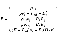
The equations we seek to solve are the usual MHD  equations. When written in conservative form, they read:

 

$$\frac{\partial \rho}{\partial t} + \vec{\nabla}\cdot (\rho \vec{v}) = 0 ,$$ (1)

$$\frac{\partial \rho \vec{v}}{\partial t} + \vec{\nabla}\cdot (\rho\vec{v}\vec{v} - \vec{B}\vec{B}) + \vec{\nabla}P_{\rm tot} =0 ,$$ (2)

$$\frac{\partial E}{\partial t} + \vec{\nabla}\cdot \left[ (E+P_{\rm tot})\vec{v}-\vec{B}(\vec{B} \cdot \vec{v}) \right] =0 ,$$ (3)

$$\frac{\partial \vec{B}}{\partial t} + \vec{\nabla}\cdot (\vec{v}\vec{B} - \vec{B}\vec{v}) = 0 .$$ (4)

Here, $\rho$ is the fluid density, $\vec{v}$ its velocity and $\vec{B}$is the magnetic field. $P_{\rm tot}$ stands for the total pressure, the sum of the thermal pressure P and the magnetic pressure:

$$P_{\rm tot}=P+\frac{\vec{B}\cdot\vec{B}}{2} ,$$ (5)

and E is the total energy of the fluid

$$E=\epsilon+\rho\frac{\vec{v}\cdot\vec{v}}{2}+\frac{\vec{B}\cdot\vec{B}}{2} ,$$ (6)

where $\epsilon$ denotes the internal energy. Unless otherwise stated, we will assume throughout this paper that the equation of state is that of a perfect gas, in which case $P=(\gamma - 1) \epsilon$.

As discussed in the introduction, this set of equations has to be completed by the solenoidal constraint, to be satisfied at all times:

$$\vec{\nabla}\cdot \vec{B} = 0.$$ (7)

As in Teyssier et al. (2006), we will use throughout this paper the CT scheme (Evans & Hawley 1988) to ensure that this condition is fulfilled to machine-roundoff precision. It simply consists in writing the induction equation in integral form:

$$\frac{\partial \Phi_{\rm s}}{\partial t}=\frac{\partial}{\par... ...B} \cdot {\rm d}\vec{S} = \oint \vec{E} \cdot {\rm d}\vec{l} ,$$ (8)

where $\vec{E}$ is the electric field defined by the relation $\vec{E}=\vec{v} {\times}\vec{B}$. While all the hydrodynamic variables (density, velocities, total energy) are located at cell centers, this approach requires the magnetic field components to lie on the cell faces. The grid structure that results is described in the following section.

2.2 The staggered mesh

In the followings, we describe our scheme using 3 dimensional coordinates x, y and z. The physical variables are discretized on a standard 3D Cartesian grid. The center of each cell is located at the position (x_i,y_j,z_k). In a given cell, faces normal to the x-direction have coordinates $x=x_{i \pm 1/2}$ and cover a surface element defined by y_j-1/2<y<y_j+1/2 and z_k-1/2<z<z_k+1/2. The coordinates of the other faces, normal to the y and z direction, can be similarly defined.

As for the Euler equations, the hydrodynamical variables (density, momentum, energy) are volume-averaged over a cell and the discretized values are defined at the cell center. For example:

$$\rho_{i,j,k}=\frac{1}{\Delta x \Delta y \Delta z} \int_{x_{i-... ...1/2}}^{z_{k+1/2}} \rho(x',y',z') {\rm d}x'{\rm d}y'{\rm d}z'.$$ (9)

Because of the staggered mesh representation, magnetic fields components are surface-averaged over the cell face to give:

$$B_{x,i-1/2,j,k}=\frac{1}{\Delta y \Delta z} \int_{y_{j-1/2}}^... ...{k-1/2}}^{z_{k+1/2}} B_x(x_{i-1/2},y',z') {\rm d}y'{\rm d}z'.$$ (10)

Here $\Delta x$, $\Delta y$ and $\Delta z$ stand for the Cartesian mesh size in each direction.

   
2.3 The Euler system

As outlined in Londrillo & Del Zanna (2000), the system of MHD equations written in Sect. 2.1 can be broken in two sub-systems. The first involved the time evolution of the cell-centered, volume-averaged variables and is reminiscent of the standard Euler equations, which includes mass, momentum and energy conservation. This set of equations, quite naturally called the "Euler system'', can be written in vectorial form

$$\frac{\partial \vec{U}}{\partial t} +\frac{\partial \vec{F}}{... ... \vec{G}}{\partial y} +\frac{\partial \vec{H}}{\partial z}=0 ,$$ (11)

where

$$\vec{U}=(\rho,\rho v_x,\rho v_y,\rho v_z, E)^{\rm T}$$ (12)

and the flux function $\vec{F}$ is given by

$$\vec{F}=\left( \begin{array}{c} \rho v_x \\ \rho v_x^2 +P_{\... ...rm tot})v_x - B_x(\vec{B} \cdot \vec{v}) \end{array} \right) .$$ (13)

The expression for $\vec{G}$ for $\vec{H}$ are completely symmetric. Integrating in space over a cell and in time between tⁿ and tⁿ⁺¹, Eq. (11) writes:

 

$$\frac{\vec{U}^{n+1}_{i,j,k}-\vec{U}^n_{i,j,k}}{\Delta t} +\frac{\... ... y}+ \frac{\vec{H}^{n+1/2}_{i,j,k+1/2}-\vec{H}^{n+1/2}_{i,j,k-1/2}}{\Delta z}=0$$ (14)

where superscripts n and n+1 refer respectively to time coordinates tⁿ and tⁿ⁺¹. $\vec{U}^n_i$ and $\vec{U}^{n+1}_i$ are the volume-averaged variables at time tⁿ and tⁿ⁺¹. The time- and surface-averaged fluxes are defined by

$$% \vec{F}_{i+1/2,j,k}^{n+1/2}= \frac{1}{\Delta t\Delta y \Delta z... ..._{z_{k-1/2}}^{z_{k+1/2}} \vec{F}(x_{i+1/2},y',z',t'){\rm d}y'{\rm d}z'{\rm d}t'$$ (15)

where $\Delta t=t^{n+1}-t^n$. Similar time and surface-average quantities are written for the fluxes G^n+1/2_i,j+1/2,k and H^n+1/2_i,j,k-1/2 appearing in Eq. (14).

In this paper, we intend to extend the well-known MUSCL-Hancock scheme (van Leer 1977; Toro 1997) to the equations of ideal MHD. When applied to the Euler equations, this method performs the conservative update of the volume-average variables $\vec{U}$ in two steps: a predictor step and a corrector step. In the former, the vector $\vec{U}$ is computed at the half time step $t^{n+1/2} = t^n + \Delta t/2$ using a Taylor expansion of the underlying hyperbolic system. It is also spatially reconstructed from the cell center to the cell faces using a piecewise linear reconstruction based on TVD slope limiters. In the predictor step, the fluxes appearing in Eq. (14) are evaluated by solving a 1D Riemann problem between the two (left and right) reconstructed states at each cell interface.

2.3.1 Cell-centered TVD slopes

The first step in the MUSCL approach is the computation of finite-difference approximation of the spatial derivatives of all cell-centered quantities. As usually done in higher order finite volume schemes, spatial derivatives are approximated using slope limiters, in order to obtain positivity preserving, non oscillatory solutions. Except for the final conservative update, we always use the primitive variables $\vec{W} = (\rho, v_x, v_y, v_z, P)^{\rm T}$ in all intermediate calculations. In addition to these 5 cell-centered variables, we need to define volume-averaged magnetic field components. We use for that purpose the average of their corresponding face-centered components

$$B^n_{x,i,j,k}=\frac{1}{2} \left( B_{x,i-1/2,j,k}^{n}+B_{x,i+1/2,j,k}^{n} \right) ,$$ (16)

and likewise for Bⁿ_y,i,j,k and Bⁿ_z,i,j,k. We finally augment the vector $\vec{W}^n$ with these 3 new components. We use in our current implementation two standard slope limiters (used in many fluid dynamics codes), the MinMod slope and the MonCen (Monotonized Central) slope (Toro 1997). The MinMod limiter is more diffusive than the MonCen limiter, so we use the latter for most applications. On the other hand, the MinMod limiter is known to ensure the positivity of the solution in multiple space dimensions. In difficult cases, we therefore switch to the MinMod slope limiter.

2.3.2 The Euler predictor step

The standard MUSCL methodology can be applied to the Euler sub-system, using the previously defined cell-centered vector $\vec{W}$. The solution is advanced in time up to t^n+1/2 using a Taylor expansion of the Euler system in non-conservative form based on the previously computed TVD slopes

$$\vec{W}^{n+1/2}_{i,j,k} = \vec{W}^n_{i,j,k} - \vec{A_x}^n_{i,j,k}... ..._{i,j,k} \left( \frac{\partial \vec{W}}{\partial z}\right)^n_{i,j,k} \Delta t/2$$ (17)

where the matrix $\vec{A_x}$ (resp. $\vec{A_y}$ and $\vec{A_z}$) is the Jacobian matrix of the flux function in the x (resp. y and z) direction, evaluated using the cell-averaged state $\vec{W}^n_{i,j,k}$. At this stage, we have cell-centered predicted states at time t^n+1/2 for the 5 Euler variables $\vec{W}^{n+1/2}_{i,j,k} = (\rho, v_x, v_y, v_z, P)^{\rm T}$. Face-centered predicted values for the magnetic field components are also computed using the method described in details in Sect. 2.4. We compute the predicted cell-centered components of the magnetic field using the average of their corresponding face-centered values. We finally augment the vector $\vec{W}^{n+1/2}_{i,j,k}$ with these 3 new cell-centered predicted variables.

2.3.3 The Euler corrector step with 1D Riemann solvers

Using the TVD slopes computed at time tⁿ, we reconstruct the primitive variables at each cell-interface, except for the longitudinal magnetic field component, since its predicted value has been already computed at the correct location (see Sect. 2.4). For example, at the two interfaces perpendicular to the x-axis, we obtain the two following reconstructed states

$$\vec{W}^{n+1/2,L}_{i+1/2,j,k} = \vec{W}^{n+1/2}_{i,j,k} + \le... ...frac{\partial \vec{W}}{\partial x}\right)^n_{i,j,k} \Delta x/2$$ (18)

$$\vec{W}^{n+1/2,R}_{i-1/2,j,k} = \vec{W}^{n+1/2}_{i,j,k} - \le... ...ac{\partial \vec{W}}{\partial x}\right)^n_{i,j,k} \Delta x/2 .$$ (19)

These states will be used as input states for 1D Riemann problems perpendicular to each interfaces. Note that for these 1D MHD Riemann problems, left and right states are defined using only 7 variables, namely the 5 Euler variables and the 2 magnetic field transverse components, thus the name "seven waves Riemann solvers''. As far as the Riemann solver is concerned, the longitudinal component of the magnetic field is assumed to be constant in time and space, in order to enforce the solenoidality constraint in one space dimension. This constant value is taken equal to the predicted value at time t^n+1/2, namely  B^n+1/2_x,i+1/2,j,k (resp.  B^n+1/2_y,i,j+1/2,k and  B^n+1/2_z,i,j,k+1/2) for the interface perpendicular to the x(resp. y and z) axis. The output of these 1D Riemann solvers are the time and surface averaged fluxes at the same interface F^n+1/2_i+1/2,j,k (resp.  G^n+1/2_i,j+1/2,k and  H^n+1/2_i,j,k+1/2). In our current implementation, we use two different Riemann solvers, namely a simple, local Lax Friedrich (LLF) solver, for which the flux is given by

$$\vec{F}_{LLF}(\vec{W}_L,\vec{W}_R)=\frac{1}{2}\left(\vec{F}_L... ...ert \lambda_{\alpha} \vert \left(\vec{U}_R - \vec{U}_L \right)$$ (20)

and the MHD  Roe solver described in Cargo & Gallice (1997) and developped by Gardiner & Stone (2005a), for which the flux can be written as

 

$$\vec{F}_{Roe}(\vec{W}_L,\vec{W}_R)= \frac{1}{2}\left(\vec{F}_L+\v... ...lambda_{\alpha}\vert \vec{L_{\alpha}} \cdot \left(\vec{U}_R - \vec{U}_L \right)$$ (21)

where $\vec{U}_L$ and $\vec{U}_R$ are the conservative state on each sides of the interface, $\vec{F}_L$ and $\vec{F}_R$ the associated fluxes, $\vec{R}_{\alpha}$and $\vec{L}_{\alpha}$ are respectively the right and left eigenmatrices of the Roe matrix and $\lambda_{\alpha}$ its eigenvalues (wave speeds).

   
2.4 The induction system

To form the full set of MHD  equations, Eq. (11) has to be completed by the induction equation, called here the induction sub-system. As for the Euler system, the induction equation can be written in conservative form by a straightforward integration in space-time

 

$$\frac{B^{n+1}_{x,i-1/2,j,k}-B^n_{x,i-1/2,j,k}}{\Delta t} - \frac{... ... + \frac{E^{n+1/2}_{y,i-1/2,j,k+1/2}-E^{n+1/2}_{y,i-1/2,j,k-1/2}}{\Delta z}=0 ,$$ (22)

with similar expressions for Bⁿ⁺¹_y and Bⁿ⁺¹_z. Here conventions are similar to the ones used in Sect. 2.3 above, except that one defines now a time- and edge-averaged electromotive force (EMF) as

$$E^{n+1/2}_{z,i-1/2,j-1/2,k} = \frac{1}{\Delta t \Delta z} \int_{t... ...\int_{z_{k-1/2}}^{z_{k+1/2}} E_z(x_{i-1/2},y_{j-1/2},z',t'){\rm d}z'{\rm d}t' ,$$ (23)

and similar expresions can be derived for E^n+1/2_x and  E^n+1/2_y. As for the Euler system, the numerical evaluation of the EMF proceeds in two steps: a predictor step followed by a corrector step. The MUSCL methodology can be extended to the induction system and this extension was extensively discussed in Teyssier et al. (2006). We recall here only the basic ingredients.

2.4.1 Face-centered TVD slopes

In order to obtain a second-order accurate and non-oscillatory solution, we need to use spatial reconstruction of the magnetic field components based on TVD slope limiters. The main difference arises because of the finite-surface representation of the magnetic field. Indeed, we need a piecewise linear representation of B_x within the y-z plane. For that purpose, we use the same TVD slopes (MinMod and MonCen) as above, using the face-averaged value of the 3 magnetic field components at time tⁿ. For B_x, we need to compute only the 2 transverse slopes $\partial B_x / \partial y$ and $\partial B_x /\partial z$. A similar property holds for B_y and B_z.

   
2.4.2 The induction predictor step

Various methods to perform the predictor step for the induction system were recently explored by Teyssier et al. (2006) for the kinematic case. These methods were referred to as Runge-Kutta, U-MUSCL and C-MUSCL. The extension of the first two to the full set of MHD equations, while possible, is computationally expensive because they require to solve one (U-MUSCL) or two (Runge-Kutta) Riemann problems in the predictive step. Moreover, the large stencil of the Runge-Kutta scheme is not compatible with the compact stencil required by our tree-based AMR implementation. For these various reasons, we decide to use only the C-MUSCL scheme in our current MHD application. It combines the nice properties of being computationnally efficient and compatible with the AMR requirements. The price to pay is a reduced stability range for the time step, since the Courant factor has to be less than $2/(\sqrt{2}+1)$, instead of 1 for the other schemes (see Teyssier et al. 2006, for details).

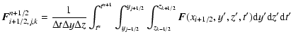
The purpose of the predictive step is to advance the solution between tⁿ and t^n+1/2 using the CT algorithm. For that, EMF need to be spatially interpolated on cell edges at time tⁿ. The idea of C-MUSCL is to do it by simple arithmetic averages of the magnetic field and velocity components. For example, the EMF E_{z,i-1/2,j-1/2,k}ⁿ is calculated by:

$$E_{z,i-1/2,j-1/2,k}^{n}=\bar{v_x}\bar{B_y}-\bar{v_y}\bar{B_x} ,$$ (24)

with

$$\bar{v_x} \frac{1}{4} \left(v^n_{x,i,j,k}+v^n_{x,i-1,j,k}+v^n_{x,i,j-1,k}+v^n_{x,i-1,j-1,k}\right) ,$$ = (25)

$$\bar{v_y} \frac{1}{4} \left(v^n_{y,i,j,k}+v^n_{y,i-1,j,k}+v^n_{y,i,j-1,k}+v^n_{y,i-1,j-1,k}\right) ,$$ = (26)

$$\bar{B_x} \frac{1}{2} \left(B^n_{x,i-1/2,j,k}+B^n_{x,i-1/2,j-1,k}\right) ,$$ = (27)

$$\bar{B_y} \frac{1}{2} \left(B^n_{y,i,j-1/2,k}+B^n_{y,i-1,j-1/2,k}\right) .$$ = (28)

This spatial reconstruction is second order in space, altough TVD slopes have not been used at that time. The EMF  E_{x,i,j-1/2,k-1/2}ⁿ, E_{y,i-1/2,j,k-1/2}ⁿ and  E_{z,i-1/2,j-1/2,k}ⁿ are then used to update the solution between t_n and t_n+1/2 using the CT algorithm (see Eq. (22)). Because only one EMF is calculated per cell edge, the predicted face-centered magnetic field ( B_x^n+1/2, B_y^n+1/2and B_z^n+1/2) satisfies the solenoidality constraint exactly. The properties of C-MUSCL and their comparison with the U-MUSCL and Runge-Kutta schemes are described in Teyssier et al. (2006). It was found that C-MUSCL behaves essentially similarly to these two other schemes, with a lower computational cost and a slightly stronger Courant condition.

2.4.3 The induction corrector step with 2D Riemann solvers

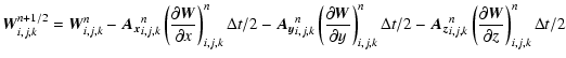
As described above, after the predictor step, we have obtained the 5 cell-centered Euler variables $\vec{W}^{n+1/2}_{i,j,k} = (\rho, v_x, v_y, v_z, P)^{\rm T}$ and the 3 face-centered magnetic field components  B_x^n+1/2, B_y^n+1/2 and  B_z^n+1/2. Using Eq. (16) at time t^n+1/2, we have also obtained the 3 predicted cell-centered components of the magnetic field. We finally augment the vector $\vec{W}^{n+1/2}_{i,j,k}$ with these 3 new cell-centered predicted variables.

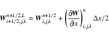
Following again the MUSCL methodology, we now need to reconstruct complete MHD  states at each cell-edge, in order to compute the EMF for the final conservative update of the magnetic field components. This reconstruction will produce 4 different states in the 4 cells adjacent to the edge. For obvious reasons, these 4 states, separated by 4 boundaries (labelled N for North, S for South, W for West and E for East) will be labelled in clockwise order by NE, SE, SW and NW.

We first reconstruct the cell-centered state to the cell edges using

$$\vec{W}^{n+1/2,NE}_{i-1/2,j-1/2,k} = \vec{W}^{n+1/2}_{i,j,k} ... ...rtial \vec{W}}{\partial y}\right)^n_{i,j,k} \frac{\Delta y}{2}$$ (29)

and similar relations that defines $\vec{W}^{n+1/2,SE}_{i-1/2,j-1/2,k}$, $\vec{W}^{n+1/2,SW}_{i-1/2,j-1/2,k}$ and $\vec{W}^{n+1/2,NW}_{i-1/2,j-1/2,k}$. Since the 2 longitudinal magnetic field components ( B_x^n+1/2 and B_y^n+1/2) are already defined at the 4 adjacent interfaces, we only need the cell-centered transverse component  B_z^n+1/2 in the above reconstruction. B_x^n+1/2 and B_y^n+1/2 are reconstructed using face-centered TVD slopes as

$$B^{n+1/2,S}_{x,i-1/2,j-1/2,k} = B^{n+1/2}_{x,i-1/2,j-1,k} + \left( \frac{\partial B_x}{\partial y}\right)^n_{i-1/2,j-1,k} \frac{\Delta y}{2}$$ (30)

$$B^{n+1/2,W}_{y,i-1/2,j-1/2,k} = B^{n+1/2}_{y,i-1,j-1/2,k} + \left( \frac{\partial B_y}{\partial x}\right)^n_{i-1,j-1/2,k} \frac{\Delta x}{2}$$ (31)

and similar relations defining B^n+1/2,N_{x,i-1/2,j-1/2,k} and  B^n+1/2,E_{y,i-1/2,j-1/2,k}. The four corner states, with 6 variables each, and the 4 longitudinal magnetic field components entirely define a 2D MHD Riemann problem, which satisfies the solenoidality constraint in a 2D sense. Londrillo & Del Zanna (2000) have shown that the EMF entering in the final Contrained Transport update should be obtained as the solution of this 2D Riemann problem, in order to obtain a stable numerical solution, with a proper upwinding of all MHD waves. While a very simple exact solution exists in the kinetic case (Teyssier et al. 2006), designing 2D Riemann solvers for the full set of MHD equations is an ambitious task that is beyond the scope of this paper. An approximate solution, proposed by Balsara & Spicer (1999) and Ziegler (2004), is based on averaging the flux given by the four adjacent 1D Riemann problems. The solution E_z^2D of the 2D Riemann problem writes in that case:

$$E^{2D}_z(\vec{W}^{NE},\vec{W}^{SE},\vec{W}^{SW},\vec{W}^{NW})$$ =

$$\frac{1}{4} ( E^{1D}_z(\vec{W}^{NW},\vec{W}^{NE}) E^{1D}_z(\vec{W}^{SW},\vec{W}^{SE})$$ +

$$+E^{1D}_z(\vec{W}^{SW},\vec{W}^{NW}) E^{1D}_z(\vec{W}^{SE},\vec{W}^{NE}) ) ,$$ + (32)

where the quantities E^1D_z stands for the solution of the 1D Riemann problems defined by the four states. This solution relies on 4 Riemann solvers per cell edges and turns out to be quite expensive. Following the ideas of Londrillo & Del Zanna (2000, 2004), we exploit the fact that in our current implementation, we use only linear Riemann solvers (namely Lax-Friedrich and Roe). In this case, the flux can be written as in Eq. (21). If we now use 2 Roe matrices, one for each direction, instead of 4, the EMF function can be written as

$$E^{2D}_z(\vec{W}^{NE},\vec{W}^{SE},\vec{W}^{SW},\vec{W}^{NW})$$ =

$$\frac{1}{4} ( E_z(\vec{W}^{NE}) + E_z(\vec{W}^{SE}) E_z(\vec{W}^{SW})+ E_z(\vec{W}^{NW}) ) \nonumber$$ +

$$- \frac{1}{2} \sum_{\alpha=1,7} \vec{R}^x_{\alpha} \vert\lambda^x_{\alpha}\vert \vec{L^x_{\alpha}} \cdot \left(\vec{U}_E - \vec{U}_W \right)$$

$$+ \frac{1}{2} \sum_{\alpha=1,7} \vec{R}^y_{\alpha} \vert\lambda^y_{\alpha}\vert \vec{L^y_{\alpha}} \cdot \left(\vec{U}_N - \vec{U}_S \right)$$ (33)

where $\vec{U}_E$, $\vec{U}_W$, $\vec{U}_N$ and $\vec{U}_S$ are averaged conservative variables defined at the interfaces of the four 1D Riemann problems. One intersesting property in the above expression is the explicit contribution of the 2 diffusive terms coming from the 2 Roe matrices. For non-linear Riemann solvers, such as HLL, it is preferable to use the 4 Riemann solvers approximation (Londrillo & Del Zanna 2004; Ziegler 2004).

2.5 The AMR scheme

The AMR algorithm used in RAMSES is described in details in Teyssier (2002) and its extension to MHD in Teyssier et al. (2006). We briefly recall the main features here. It is a tree-based AMR code originally designed for cosmological applications. The data structure is a "Fully Threaded Tree'' (Khokhlov 1998). The grid is divided into groups of 8 cells, called "octs'', that share the same parent cell. Each oct has access to its parent cell address in memory, but also to neighboring parent cells. When a cell is refined, it is called a "split'' cell, while in the opposite case, it is called a "leaf'' cell. The computational domain is always defined as the unit cube, which corresponds in our terminology to the first level of refinement in the hierarchy $\ell = 1$. The grid is then recursively refined up to the minimum level of refinement  $\ell_{\rm min}$, in order to build the coarse grid. This coarse grid is the base Cartesian grid, covering the whole computational domain, from which adaptive refinement can proceed. This base grid is eventually refined further up to some maximum level of refinement  $\ell_{\rm max}$, according to some user defined refinement criterion. When  $\ell_{\rm max}=\ell_{\rm min}$, the computational grid is a traditional Cartesian grid, for which the previous scheme apply without any modification. When refined cells are created, however, some issues specific to AMR must be addressed.

2.5.1 Divergence-free prolongation operator

When a cell is refined, eight new cells (i.e. a new "oct'') are created for which new cell-centered variables and new magnetic field components are needed. This operation is usually referred to as the "prolongation operator''. The traditional approach relies on a conservative interpolation of the 5 cell-centered conservative variables $\vec{U}=(\rho,\rho v_x,\rho v_y,\rho v_z, E)^{\rm T}$. For the face-centered variables, each of the six faces of the parent cell are split into 4 new fine faces. Three new faces, at the center of the parent cell, are also split into four new children faces. The resulting magnetic field components, fine or coarse, need to satisfy the divergence-free constraint in integral form.

This critical step has been solved by Balsara (2001) and Tóth & Roe (2002) in the CT framework. We recommend both of these articles for a detailed description of the method. The idea is to used slope limiters to interpolate the magnetic field component inside each parent face, in a flux-conserving way, and then to use a 3D reconstruction, which is divergence-free in a local sense inside the whole cell volume, in order to compute the new magnetic field components for each central children faces. In our case, the same slope limiters as in the Godunov scheme (MinMod or MonCen) can be used.

This prolongation operator is used to estimate the magnetic field in newly refined cells, but also to define a temporary "buffer zone'', two "ghost cells'' wide, that set the proper boundary for fine cells at a coarse-fine level boundary. This is the main reason why compact stencils are needed for the underlying Godunov scheme.

2.5.2 Magnetic flux corrections

The other important step is to define the reverse operation, when a split cell is de-refined, and becomes a leaf cell again. This operation is usually called the Restriction Operator in the multigrid terminology. The solenoidality constraint needs again to be satisfied, which translates into conserving the magnetic flux. The magnetic field component in the coarse face is just the arithmetic average of the 4 fine face values. This is reminiscent of the "flux correction step'' for the Euler system (Teyssier 2002; Berger & Oliger 1984; Berger & Colella 1989).

2.5.3 EMF corrections

The "EMF correction step'' is more specific to the induction equation. For a coarse face which is adjacent, in any direction, to a refined face, the coarse EMF in the conservative update of the solution needs to be replaced by the arithmetic average of the two fine EMF vectors. This guarantees that the magnetic field remains divergence-free, even at coarse-fine boundaries.

   
3 Numerical tests in 1D

3.1 Non-linear Alfvén wave test

	Figure 1: Amplitude ( upper panel) and phase velocity ( lower panel) of the circularly polarized Alfvén wave as a function of time. The full lines display result using a Roe solver whereas the dotted lines show results obtained with a Lax-Friedrich solver. The resolutions are from top to bottom, 100, 30 and 10 grid points per wavelength.
Open with DEXTER

The first test we present is the propagation of non-linear circularly polarised Alfvén waves. Such waves, which are exact solution of the MHD equations, propagate in a gas of uniform density, $\rho_0$ and along a uniform magnetic field, B_0z. They are given by: $B_x = B_\perp \cos(\omega t - k z)$, $B_y = B_\perp \sin(\omega t - k z)$, $V_x = V_\perp \cos(\omega t - k z)$, $V_y = V_\perp \sin(\omega t - k z)$ where $\omega / k = B_{0z} / \sqrt{4 \pi \rho_0}$ and $B_\perp / V_\perp = \sqrt{4 \pi \rho_0}$.

We have simulated the propagation of these waves on a uniform grid, for $B_{0z}=\sqrt{4 \pi}$, $B_\perp=\sqrt{\pi}$, and k=0.1. This leads to a wave period equal to 0.1. The agreement between the analytical and numerical solutions depends on the numerical resolution. Figure 1 displays the wave amplitude ( upper panel) and phase velocity (lower panel) as a function of time for the Roe and Lax-Friedrich solvers and different resolutions, namely 10, 30 and 100 points per wavelength. With 10 grid points per wavelength, the amplitude quickly decays because of numerical dissipation and in about 5 wave periods, the amplitude of the waves is only 40$\%$ of its initial value. With 30 and 100 grid points per wavelength the agreement is much better and almost no decay has occurred even after 50 wave periods in the latter case. In the lower panel, the wave velocity is also seen to agree better and better with its theoretical value, v_w=1, as the resolution is increased (note that for 100 grid points, the wave velocity obtained with the Roe solver is not represented as it is indistinguishable from the Lax-Friedrich results). As expected the Roe solver leads to slightly better results in both cases than the Lax-Friedrich solver.

3.2 MHD shock tube test

	Figure 2: Solution to the MHD shock tube showing the density as a function of x, obtained with RAMSES when $\alpha =\pi$. The code uses 400 grid points in that case and the Roe Riemann solver.
Open with DEXTER

An interesting application of the AMR scheme is the study of the development of compound waves in shock tube calculations. It has been analysed with finite volume schemes by Torrilhon (2004), through the analysis of the MHD shock tube whose initial state is:

$$\vec{W^L} (1,0,0,0,1,1,1,0)^{\rm T}$$ = (34)

$$\vec{W^R} (0.2,0,0,0,0.2,1,\cos \alpha,\sin \alpha)^{\rm T}$$ = (35)

where $\vec{W}=(\rho,v_x,v_y,v_z,P,B_x,B_y,B_z)^{\rm T}$. When $\alpha =\pi$, there are two solutions to the Riemann problem: the first is regular, which means that it contains only shocks and contact discontinuities. The second, however, features a compound wave which is a composition of an Alfvén and a slow wave. Torrilhon (2004) showed that finite volume schemes converge toward the second. When $\alpha$ is different from $\pi$, the solution is regular and should only contain shocks and contact discontinuities. However, Torrilhon (2004) found that finite volume codes still tend to exhibit the compound wave for low and moderate resolutions. The solution converges toward the regular solution only when very large resolutions are used.

Here, we use RAMSES to illustrate how the AMR scheme can help to solve this problem. Figure 2 shows the density vs. position when $\alpha =\pi$ at time t=0.4. The grid is composed of 400 cells evenly distributed between -1 and 1.5. The AMR is switched off in this first run. The compound wave is clearly visible at $x\simeq-0.25$. The whole solution looks identical to previous results published in the literature with similar codes (Ryu & Jones 1995; Londrillo & Del Zanna 2000; Cargo & Gallice 1997).

Figure 3: Zoom on the region in which the compound wave develops when $\alpha =3$. Black curves are obtained on a uniform grid. From top to bottom (at $x \sim -0.24$), they correspond to 800, 1200, 1600, 2000, 3000, 5000, 10 000 and 20 000 grid points respectively. The red curve was calculated after switching on the AMR scheme and using a similar CPU time as for the 20 000 grid points curve. Its maximum resolution is equivalent to using about 106 cells on a uniform grid and show a dramatic improvement toward the regular solution.

Open with DEXTER

	Figure 4: Complete solution of the MHD shock tube when $\alpha =3$, with the AMR scheme turned on. The solid line is a plot of the density as a function of position while the dashed line (whose scale is given on the right axis) illustrates the level of refinement the code uses for each cell.
Open with DEXTER

Taking now $\alpha =3$ and computing the solution of the MHD shock tube on a uniform grid, we also found that the compound wave remains for low resolution as described by Torrilhon (2004). This is illustrated in Fig. 3, which is a zoom on the structure of the solution in the neighbourhood of the compound wave. The black lines are computed on a uniform grid and correspond to increasing resolution. Namely, from top to bottom (at $x \sim -0.24$), the number of cells are 800, 1200, 1600, 2000, 3000, 5000, 10 000 and 20 000. The red line shows the result of the same model computed using the AMR scheme with a refinement strategy based on the magnitude of the gradient of all 7 flow variables. The finest resolution in this run is equivalent to having 10⁶ cells on a uniform grid. We found the result of this model to be almost indistinguishable from the regular solution (remember that this is the ONLY physical solution to this problem). Interestingly, this is not the case for the uniform runs. Even though the compound wave is seen to gradually disappear as the resolution is increased, features departing from the correct solution are still observed even when 20 000 grid zones are used. This illustrates the extremely large resolution needed to accurately calculate the solution of this problem and shows the interest of using AMR. Indeed, the AMR run used only 10 000 cells for the same equivalent resolution as 10⁶ grid cells, which corresponds to a gain of about 2500 in CPU time.

The complete solution of the AMR model is shown in Fig. 4. As is Fig. 2, the solid line represents the density as a function of position. The dashed line shows the corresponding refinement level. It scale is indicated on the right axis. As expected, the grid is highly refined at the location of the shocks and contact discontinuities. It is important to understand that the AMR is not just a fancy tool for this test, but is actually essential to solve it properly. One might indeed think that increasing the order of the numerical scheme would help to converge to the regular solution at lower resolution. Torrilhon & Balsara (2004) actually showed that the improvement when using third or fourth order WENO schemes is small. This is because the accuracy of any such schemes breaks down to first order close to discontinuities, which is precisely where the compound wave lies.

   
4 Numerical tests in 2D

4.1 Advection of a magnetic loop

	Figure 5: Time history of the magnetic energy in the magnetic loop advection test. The different curves are obtained using the Roe Riemann solver ( solid line) and the Lax-Friedrich solver ( dashed line).
Open with DEXTER

As a first 2D test, we now consider the simple advection of a magnetic loop that has recently been proposed by Gardiner & Stone (2005a). It simply consists in the evolution of a weak magnetic field in an initially uniform velocity field. Since the thermal pressure is much larger than the magnetic pressure, the magnetic field can be considered as a passive tracer advected in a time independent flow. The initial setup is exactly the same as in Gardiner & Stone (2005a) and Teyssier et al. (2006). The velocities are set up to v_x=2, v_y=1 and v_z=0. The initial magnetic field is such that B_z=0, while the components B_x and B_y are defined using the z-component of the potential vector $\vec{A}$ ( $\vec{B}= \vec{\nabla} {\times}\vec{A}$):

$$A_z = \left\{ \begin{array}{cc} A_0(R-r) & {\rm for~} r < R ,\\ 0 & \rm {otherwise} , \end{array}\right.$$ (36)

with A₀=10^-3, R=0.3 and $r=\sqrt{x^2+y^2}$. The computational domain is defined as -1<x<1 and -0.5<y<0.5. There are 128cells in the first direction and 64 in the second. The solution is evolved between t=0 and t=2 and we analyzed the results obtained by our scheme using the MonCen slope limiter, comparing explicitly the Roe solver to the local Lax-Friedrich solver.

A simple way to evaluate the efficiency of the scheme is to compare the time history of the magnetic energy E_m. This is done in Fig. 5, where E_m is represented as a function of time for the Roe solver (solid line) and for the Lax-Friedrich solver (dashed line). We first note that the results are very similar to those published by Gardiner & Stone (2005a). This demonstrates that, using only TVD linear reconstruction, our scheme provides comparable accuracy to the piecewise parabolic scheme of Gardiner & Stone (2005a). As expected, the Lax-Friedrich solver is more dissipative, while the results obtained using the Roe solver exactly reproduce the results obtained in the pure advection case (Teyssier et al. 2006), to which we refer the reader for more details, especially regarding the AMR scheme.

4.2 The Orszag-Tang vortex

	Figure 6: Snapshot of the density at time t=0.5 resulting from the Orszag-Tang test. The grid is uniform and composed of 5122 cells. The result is computed using the Roe Riemann solver and the C-MUSCL predictive step.
Open with DEXTER

One of the most well-known 2D MHD test is the Orszag-Tang test. The initial condition of the flow create a vortex that is unstable and quickly breaks down into turbulence. Although no analytical solution is known for this test, it has been so widely documented in the literature that it is now very useful as a first 2D benchmark for a code.

The initial state is defined as

$$\rho \gamma P_0 ,$$ = (37)

$$\vec{v} (-\sin 2\pi y,\sin 2\pi x) ,$$ = (38)

$$\vec{B} (- B_0 \sin 2\pi x,B_0 \sin 4\pi y) .$$ = (39)

The different parameters are defined by

$$\gamma=\frac{5}{3} , ~ P_0=\frac{5}{12\pi} \ \ {\rm and }~~B_0=\frac{1}{\sqrt{4\pi}} \cdot$$

The grid extends from 0 to 1 in both directions and we use 512² cells uniformly distributed over the computational domain. The solution is evolved between t=0 and t=0.5 using the Roe solver and the MonCen slope limiter. The density distribution in the (x,y) plane at the end of the simulation is shown in Fig. 6. The agreement between our result and previous published work is excellent (Ryu et al. 1998; Londrillo & Del Zanna 2000). The complex pattern of interacting waves is perfectly recovered.

4.3 The current sheet

	Figure 7: Time evolution of the magnetic field lines during the current sheet test. The calculation was performed on a uniform grid composed of 2562 cells, using the Roe solver and the MonCen slope limiter. From top left to bottom right, the snapshots corresponds successively to times t=0,0.5,1,1.5,2,2.5,3, 3.5 and 4. The entire figure can be compared to Fig. 12 of Gardiner & Stone (2005a).
Open with DEXTER

Gardiner & Stone (2005a) recently described a 2D test that follows the time evolution of a current sheet created by a magnetic field discontinuity. Reconnection occurs at the location of the discontinuity. Because no explicit dissipation is included in the code, the entire evolution is driven by the numerical resisitivity of the scheme, and, as such, is sensitive to every details of the algorithm. The initial setup is described in the followings.

Figure 8: This figure compares the magnetic field lines obtained at time t=2 for high-resolution runs ( bottom) and low-resolution runs ( top), as well as for the Roe solver ( right) and the local Lax-Friedrich solver ( left). Both low and high-resolution runs were performed using the AMR scheme: $l_{\rm min}=5$ for the former and $l_{\rm min}=10$ for the latter. The refinement strategy is detailed in the text.

Open with DEXTER

The computational domain lies in the domain $0 \leq x \leq 2$ and $0 \leq y \leq 2$ and is divided in 256 uniform cells in each directions. At time t=0, density and pressure are uniform: $\rho=1$and P=0.1. The magnetic field components vanish in the x and z direction and B_y is defined by

$$B_y= \left\{ \begin{array}{ll} -1 & {\rm if}~\vert x-1\vert \leq 0.5 , \\ +1 &{\rm otherwise} . \end{array} \right.$$ (40)

Similarly, v_y=v_z=0 and $v_x=v_0 \sin~(\pi y)$.

	Figure 9: This figure shows a zoom on the bottom left magnetic island for the high-resolution run with the Roe solver at time t=3. On the left, only octs boundaries are plotted to clarify the visualization of the AMR grid. On the right, a grey scale image of the thermal pressure is shown, with strong transverse shock-waves clearly visible as sharp discontinuities.
Open with DEXTER

We first present our numerical results using the Roe solver with the MonCen slope limiter. They are represented in Fig. 7. The magnetic field lines are plotted at times t=0, 0.5, 1, 1.5, 2, 2.5, 3, 3.5and 4. As reported by Gardiner & Stone (2005a), magnetic islands form, grow and eventually merge with each other. At the end of the simulation, four islands are clearly visible at the location of each discontinuity. A direct comparison between our results and Fig. 12of Gardiner & Stone (2005a) shows that both codes agree almost perfectly up to time t=2.5. On the other hand, at later time, no strong evolution is observed in our case, while for the ATHENA code, the flow symmetry is broken and the two islands merge into a single large one (Gardiner & Stone 2005a). As discussed above, this difference is an indication that both codes, although very similar, have different dissipative properties.

The next step is to test our AMR scheme in 2D: we perform the same exact simulation, except that now we use a base grid of n_x=n_y=32, which corresponds to $\ell_{\rm min}=5$, with 3 additional levels of refinement, so that $\ell_{\rm max}=8$. The formal resolution is thus equivalent to the first test with a regular Cartesian grid. We use a refinement strategy based on the gradient of the thermal pressure:

$$\frac{\max \left( \left\vert \Delta_x P \right\vert, \left\vert \Delta_y P \right\vert \right) } {P}> 0.05 ,$$ (41)

associated with a similar criterion based on B_y. In Fig. 8, we show the magnetic field lines at time t=2 obtained with the Roe solver (upper right plot): it is indistinguishable from the previous result obtained with a Cartesian grid. For sake of comparison, we have also compared the result obtained at t=2 with the Lax-Friedrich solver (upper left plot): it is now completely different. Due to the increased numerical diffusivity of the Lax-Friedrich solver, the tiny magnetic islands, that move up and down from the center of the image, have not yet merged to their final position. Moreover, with the Roe solver, we also obtain a static magnetic island at the position of the flow stagnation point. This static island is absent from the Lax-Friedrich solution. As anticipated, this test is highly discriminant of the dissipative properties of numerical schemes.

In order to study the convergence of each solution, we take advantage of the speed-up provided by the AMR grid to perform additional high-resolution simulation. Using the same refinement strategy, we now set $\ell_{\rm max}=10$, so that the formal resolution is now n_x=n_y=1024. We present in Fig. 9 the resulting AMR grid, together with a grey-scale image of the thermal pressure. We see that AMR cells are optimally distributed in order to properly sample the current sheet, as well as sharp MHD waves propagating perpendicular to the current sheet. The results obtained at t=2using both Riemann solvers are shown at the bottom plots of Fig. 8. The Roe solution has not changed when compared to its low-resolution counterpart. This demonstrates that the lower numerical dissipation of the Roe solver allows a faster convergence of the numerical solution. Interestingly, the Lax-Friedrich high-resolution solution has also converged toward the same solution, except for the static magnetic island at the flow stagnation point. This demonstrates that using AMR can provide fast convergence towards the true solution, even with a rather dissipative scheme. On the other hand, the static island in the center of the flow seems to be highly sensitive to the details of the scheme. As opposed to Lax-Friedrich, the Roe solver has the interesting property that for a static velocity field, the numerical dissipation vanishes exactly. The difference between the 2 solvers is therefore maximized at the stagnation point, where both schemes are converging towards 2 different solutions, even at our highest resolution. This peculiar behavior is due to the fact that this reconnection problem is performed without any physical resistivity. It should be therefore considered only as an interesting numerical test, rather than a true physical application.

   
5 Astrophysical applications in 3D

To illustrate the possibilities of RAMSES, we present in this section two 3D tests of astrophysical significance: the development of Magneto-Rotational Instability (MRI) and the formation of a magnetized molecular core.

5.1 The magnetorotational instability

The development of MHD turbulence resulting from the growth of the MRI is likely to be at the origin of an efficient radial transport in accretion disks. This instability has been extensively studied using finite difference codes like ZEUS (Hawley et al. 1995); our goal is here to compare the results of RAMSES with those obtained in earlier studies during the last decade.

The MRI is a linear instability that was first discovered in the 60s (Velikhov 1959; Chandrasekhar 1961) before being applied to accretion disks theory by Balbus & Hawley (1991). It operates in rotating flows threaded by a weak magnetic field when the angular velocity decreases outward. Numerical simulations applied to accretion disks have shown that the linear growth of the instability is followed by MHD turbulence that transports angular momentum outward in the disk, thereby solving a long standing issue in accretion disk theory (see Balbus & Hawley 1998, for a review). One subclass of these simulations has been realised using the so-called shearing box approximation. It is a local expansion of the dynamical equation in a Cartesian box around a particular radius of the accretion disk (Goldreich & Lynden-Bell 1965). The interest of this local approach is that it is able to capture the dynamics of the accretion disk and enables large resolution to be achieved at the same time. With such a model, the properties of the MHD turbulence can be rather well studied.

So far, most of the shearing box simulations have been done using artificial viscosity codes, like ZEUS (Hawley et al. 1995), NIRVANA (Papaloizou et al. 2004) or the Pencil Code (Brandenburg et al. 1995). Recently, Gardiner & Stone (2005b) applied the ATHENA code to the same problem. They found that using a Riemann solver make little difference.

We have implemented the shearing box model in RAMSES. To do so, two main modifications have to be made. First, the inertial terms appearing in the equations are treated as source terms. Second, the boundary conditions need to be adapted to the model. They are periodic in y and z, which respectively correspond to the $\phi$ and z coordinates of the standard cylindrical coordinates. The boundary conditions in x (the equivalent of R in cylindrical coordinates) are the so-called shearing boundary conditions widely discussed in the literature (Gardiner & Stone 2005b; Hawley et al. 1995).

	Figure 10: Structure of the flow in the (x,z) plane after 60 orbits. The arrows shows the poloidal velocity field overplotted on gray scale contours of the y-component of the magnetic field. Because of the growth of the MRI, the entire flow has become turbulent.
Open with DEXTER

	Figure 11: Time history of the volume averaged Maxwell stress tensor normalized by pressure, obtained in the shearing box model. The solid line was computed using RAMSES and the dashed line was calculated using ZEUS. Both models use exactly the same set of parameters. Both shows sustained MHD turbulence and a similar amount of angular momentum transport.
Open with DEXTER

	Figure 12: Three timesteps illustrating the hydrodynamical collapse.
Open with DEXTER

The initial conditions of our runs are those of the standard shearing box model. The initial density is uniform and equal to unity everywhere. The velocity is such that

$$\vec{v}=\left( \begin{array}{c} 0 \\ -q \Omega_0 x \\ 0 \end{array}\right),$$ (42)

with q=1.5 and $\Omega_0=10^{-3}$. The equation of state is isothermal: $P=\rho c_{0}^2$, with c₀=10^-3. The initial magnetic field is initially purely vertical and its intensity varies sinusoidally with x such that the total net flux threading the computational domain vanishes:

$$B_z=B_0 \sin 2 \pi x .$$ (43)

B₀ is calculated such that the ratio $\beta$ between the volume averaged thermal to magnetic pressure equals 400. The uniform grid satisfies $-0.5 \leq x \leq 0.5$, $0 \leq y \leq 2\pi y$ and $-0.5 \leq z \leq 0.5$. The resolution is (N_x,N_y,N_z)=(32,100,32). We ran the model with RAMSES, using the Roe Riemann solver and the MonCen slope limiter.

	Figure 13: Two timesteps illustrating the magnetized collapse. The upper panels display the equatorial density and velocity field whereas bottom panels displays the density in x-z plane. The calculation is performed with the Lax-Friedrich solver.
Open with DEXTER

At t=0, small random velocities are superposed on the initial state. The model is evolved during 100 orbital periods T₀, where $T_0=2\pi/\Omega_0$. During the first five orbits, the magnetic energy is observed to grow. A measure of the growth rate of the instability $\sigma$ during that period gives $\sigma \sim 0.55 \Omega$. It is difficult to compare this growth rate with the results of linear theory: since the vertical magnetic field varies with x, its growth rate does not correspond to that of a single normal mode. Nevertheless, we expect the volume averaged evolution of the magnetic field to be dominated by the growth of the field at the position where its strength is initially the largest. This is confirmed by a visual inspection of the structure of the flow during that phase, which also indicates that the associated wavelengths in the radial and vertical direction are respectively equal to H and H/2. The results of linear theory (Balbus & Hawley 1991) predicts that $\sigma_{\rm th}=0.55 \Omega$ in that case. Although there is good agreement between $\sigma$ and  $\sigma_{\rm th}$, we want to emphasize that the treatment presented here is only approximate. It nevertheless gives confidence in the results of the numerical simulation.

	Figure 14: Same as Fig. 13 except that the calculation has been carried out with the Roe solver.
Open with DEXTER

When nonlinear effect becomes important, the magnetic energy reaches a peak and start to decline as the whole flow breaks down into turbulence, before levelling to a quasi steady state it keeps until the end of the simulation. The turbulent nature of the disk is illustrated in Fig. 10. It shows the structure of the flow in the (x,z) plane after 60 orbits. The arrows represent the poloidal velocity field and are overplotted on gray scale contours of B_y, which is the dominant component of the magnetic field. In order to better quantify the strength of the turbulence, we plot in Fig. 11 the time history of the volume averaged Maxwell stress tensor, normalised by the mean thermal pressure P₀:

$$T_{r\phi}^{\rm Max}=-\frac{\langle B_x B_y \rangle}{P_0} ,$$ (44)

where $\langle . \rangle$ denotes a volume average. The solid line in Fig. 11 was obtained with RAMSES. As a comparison, the dashed line shows the same quantity obtained with ZEUS for the same model (we note that the growth rate measured during the linear phase in that case was found to be identical to that obtained with RAMSES). The two curves are in good agreement with each other, even if there is a tendency for RAMSES to display some more activity. Indeed, time averaging the curves presented in Fig. 11 between 40 and 100 orbits, we obtained mean values and rms deviation for the Maxwell stress tensor equal to $(6.6 \pm 1.5) \times 10^{-3}$ with RAMSES and equal to $(3.9 \pm 1.3) \times 10^{-3}$ with ZEUS. It is worth noting that the (small) difference between these two values may not be significant as it is an effect of the different dissipative properties of the codes: turbulence is driven on large scales by the MRI and damps on small scales due to numerical dissipation. The precise saturated value of the Maxwell stress results from a balance between these two.

5.2 Magnetized cloud core collapse

Here we present another 3D test of astrophysical significance: the magnetized collapse of a dense prestellar core. In this problem the AMR scheme is very useful since the density varies over 8 orders of magnitude and the spacial scale, which is about the Jeans length, varies over 3-4 orders of magnitude.

Such calculations in the hydrodynamical case have been performed by several authors using either SPH methods (e.g. Hennebelle et al. 2004) or grid based method (e.g. Matsumoto & Hanawa 2003). In the magnetized case, much fewer 3D calculations have been carried out using SPH (Hosking & Whitworth 2004), nested grid (Machida et al. 2005a,b; Banerjee & Pudritz 2006) or an AMR implementation (Ziegler 2005).

In order to do a precise comparison, we adopt the same initial conditions as Hosking & Whitworth (2005) and Ziegler (2005). The cloud has initially a uniform density of $\rho = 4.8 \times 10^{-18}$ g cm^-3, a temperature of 10 K and a radius of $R_{\rm c}=0.015$ pc. The total mass is equal to one solar mass and the initial ratio of thermal to gravitational energy is about 0.35. The cloud is initially in solid body rotation with angular velocity $\omega = 4.25 \times 10^{-13}$ s^-1 leading to an initial ratio of rotational to gravitational energy of about 0.45. To induce fragmentation, an m=2 perturbation on the density field with an amplitude of 10$\%$ has been setup initially. The magnetic field is initially uniform and parallel to the rotation axis. We use the same barotropic equation of state as Hosking & Whitworth (2005), namely $P = C_{\rm s}^2 \rho \times (1 + (\rho / \rho_{\rm crit})^{4/3})^{1/2}$ with $\rho_{\rm crit}=10^{-13}$ g cm^-3. All calculations have initially 64³ cells and uses 8 additional AMR levels. The refinement criteria is based on the Jeans length which is numerically described by at least 10 cells.

5.2.1 Hydrodynamical collapse

Figure 12 displays three snapshots of the hydrodynamical case performed with the Lax-Friedrich solver. The equatorial density field is displayed and the arrows show the velocity field. The top panel is very similar to the second panel of Fig. 8 of Ziegler (2005). Both spiral patterns have approximately the same size and the same orientation. Timing is also very similar (agreement within about 5$\%$ of accuracy). The result compares well to the SPH calculation of Hosking & Whitworth (2005) shown in their Fig. 2 (bottom-right panel). The second panel of Fig. 12 appears to be similar to the bottom-left panel of Fig. 3 of Hosking & Whitworth (2005). In both cases about 5 fragments have formed located approximately at the same position in both simulations. The third panel shows the density field 0.01 Myr after the time of the second panel which is comparable to the timeshift between left-bottom and right-bottom of Fig. 3 of Hosking & Whitworth (2005). The agreement is less good than for earlier time. Our results remain symmetric which is not the case for the Hosking & Whitworth's results.

5.2.2 MHD collapse

In this section we present results for the MHD collapse. The intensity of the magnetic field is such that the cloud mass-to-flux ratio is twice the critical mass-to-flux ratio. This corresponds to the first MHD case studied by Ziegler (2005).

Figure 13 shows results for a calculation performed with the Lax-Friedrich solver whereas Fig. 14 shows results obtained with the Roe solver. Upper panels of Figs. 13 and 14 display the equatorial density field whereas bottom panels display the density in the x-z plane. Left panels display results at a time close to the first panel of Fig. 10 of Ziegler (2005). Right panels display results about 0.01 Myr later.

In his simulation, Ziegler reports the formation of a binary having a separation at time $t \simeq 1.44 t_{\rm ff}$ of about 0.06 $R_{\rm c}$ where  $t_{\rm ff}$ is the freefall time. As shown in Fig. 13, there are no binaries with the Lax-Friedrich solver. There is also a shift in time (of about $3\%$) since the collapse occurs slightly later than $1.44 t_{\rm ff}$. On the contrary, as shown in Fig. 14, in the simulation performed with the Roe solver, a binary forms at time $t=1.45 t_{\rm ff}$ although we find a separation of 0.03 $R_{\rm c}$ instead of 0.06 $R_{\rm c}$. Ziegler reports also another case with stronger magnetic field for which the mass-to-flux ratio is 1.2 times the critical mass-to-flux ratio. In this case he finds no binary. We have also performed this simulation (not displayed here for conciseness) and we confirm the absence of binary. Although the formation of the binary appears to be a good numerical test, it should be said that it is somehow physically artificial since it relies on initial conditions for which the density field is perturbed but not the magnetic field. As a result, the magnetic Jeans mass at the density maximum is lowered, thus making the perturbation very unstable. Indeed we have performed a simulation in which the m=2 perturbation has been applied to the magnetic field as well. In this case, instead of a binary, we find two very shallow local maxima.

Right panels of Fig. 14 show that the two fragments have merged leaving a single central fragment. This is an important difference with the hydrodynamical case in which five fragments have been found (although further evolution reveals that two of these fragments merge with the central one). Another important departure from the hydrodynamical case is the presence of strong outflows (right-bottom panel). There are very similar to the outflows shown in Machida et al. (2005b). Outflows are also obtained with the Lax-friedrich solver (right-botton panel of Fig. 13) although the flow structure is slightly different. With the Roe solver, the velocity field along the z-axis vanishes whereas this is not the case with the Lax-Friedrich solver. The disk appears to be thicker with the Lax-Friedrich solver than with the Roe solver.

We conclude that RAMSES-MHD is able to reproduce quantitatively results obtained by various authors including fragmentation and outflows. Significant differences appear between results obtained with the Lax-Friedrich and the Roe solvers although the former is able to reproduce the main features of the flow.

   
6 Conclusion and perspectives

In this paper, we have presented an extension of RAMSES to MHD. The algorithm is based on the MUSCL-Hancock approach already used in the hydrodynamic version of RAMSES (Teyssier 2002). The induction equation is evolved in time using the standard CT scheme (Evans & Hawley 1988). To do so, time averaged EMFs are computed on cell edges by solving a 2D Riemann problem, as described in Londrillo & Del Zanna (2000). Several tests are presented that illustrate the properties and robustness of the code. In particular, we show that the AMR scheme implemented in RAMSES can be crucial to describe accurately the propagation of some unusual waves peculiar to MHD like the compound waves.

We also demonstrate the versatility of RAMSES by studying two problems of astrophysical significance: the development of MHD turbulence in accretion disk and the collapse of dense core in the interstellar medium. In both cases, we report results that are consistent with previous studies published in the literature. These two applications show that RAMSES is well suited to study a wide variety of problems involving MHD in astrophysics.

In future studies, several improvements will now be investigated. It will be particularly useful, for example, to develop a proper 2D Riemann solver to calculate the time averaged EMFs, instead of making linear combination of 1D solvers as it is done now. Nonlinear Riemann solvers could also be implemented, like HLLC (Miyoshi & Kusano 2005) for example. Obviously, an extension to curvilinear coordinates would also be very interesting, particularly for applications involving accretion disks or galaxies. Finally, it will be necessary in some cases to go beyond the ideal MHD framework and to implement new physics like ohmic dissipation or ambipolar diffusion.

Acknowledgements

The authors thank Emmanuel Dormy and Stéphane Colombi for useful discussions. Some of the simulations presented in this paper were performed on the QMUL High Performance Computing Facility purchased under the SRIF initiative and at CCRT, the CEA supercomputing center.

References

• Balbus, S., & Hawley, J. 1991, ApJ, 376, 214 [NASA ADS] [CrossRef] (In the text)
• Balbus, S., & Hawley, J. 1998, Rev. Mod. Phys., 70, 1 [NASA ADS] [CrossRef] (In the text)
• Balsara, D. S. 2001, J. Comput. Phys., 174, 614 [NASA ADS] [CrossRef] (In the text)
• Balsara, D. S., & Spicer, D. S. 1999, J. Comput. Phys., 153, 671 [NASA ADS] [CrossRef] (In the text)
• Banerjee, R., & Pudritz, R. 2006, ApJ, 641, 949 [NASA ADS] [CrossRef] (In the text)
• Berger, M. J., & Colella, P. 1989, J. Comput. Phys., 82, 64 [NASA ADS] [CrossRef]
• Berger, M. J., & Oliger, J. 1984, J. Comp. Phys., 53, 484
• Brackbill, J. U., & Barnes, D. C. 1980, J. Comput. Phys., 35, 426 [NASA ADS] [CrossRef] (In the text)
• Brandenburg, A., & Dobler, W. 2002, Comput. Phys. Commun., 147, 471 [NASA ADS] (In the text)
• Brandenburg, A., Nordlund, A., Stein, R. F., & Torkelsson, U. 1995, ApJ, 446, 741 [NASA ADS] [CrossRef] (In the text)
• Cargo, P., & Gallice, G. 1997, J. Comput. Phys., 136, 446 [NASA ADS] [CrossRef] (In the text)
• Chandrasekhar, S. 1961, Hydrodynamic and hydromagnetic stability, International Series of Monographs on Physics (Oxford: Clarendon)
• Crockett, R. K., Colella, P., Fisher, R. T., Klein, R. I., & McKee, C. F. 2005, J. Comput. Phys., 203, 422 [NASA ADS] [CrossRef] (In the text)
• Dedner, A., Kemm, F., Kröner, D., et al. 2002, J. Comput. Phys., 175, 645 [NASA ADS] [CrossRef] (In the text)
• Evans, C., & Hawley, J. 1988, ApJ, 33, 659 [NASA ADS] [CrossRef] (In the text)
• Falle, S. A. E. G. 2002, ApJ, 577, L123 [NASA ADS] [CrossRef] (In the text)
• Gardiner, T. A., & Stone, J. M. 2005a, J. Comput. Phys., 205, 509 [NASA ADS] [CrossRef] (In the text)
• Gardiner, T. A., & Stone, J. M. 2005b, ArXiv Astrophysics e-prints (In the text)
• Goldreich, P., & Lynden-Bell, D. 1965, MNRAS, 130, 125 [NASA ADS] (In the text)
• Hawley, J. F., Gammie, C. F., & Balbus, S. A. 1995, ApJ, 440, 742 [NASA ADS] [CrossRef] (In the text)
• Hennebelle, P., Whitworth, A. P., Cha, S.-H., & Goodwin, S. P. 2004, MNRAS, 348, 687 [NASA ADS] [CrossRef] (In the text)
• Hosking, J. G., & Whitworth, A. P. 2004, MNRAS, 347, 1001 [NASA ADS] [CrossRef] (In the text)
• Khokhlov, A. M. 1998, J. Comput. Phys., 143, 519 [CrossRef] (In the text)
• Londrillo, P., & Del Zanna, L. 2000, ApJ, 530, 508 [NASA ADS] [CrossRef] (In the text)
• Londrillo, P., & Del Zanna, L. 2004, J. Comput. Phys., 195, 17 [NASA ADS] [CrossRef] (In the text)
• Matsumoto, T., & Hanawa, T. 2003, ApJ, 595, 913 [NASA ADS] [CrossRef] (In the text)
• Miyoshi, T., & Kusano, K. 2005, J. Comput. Phys., 208, 315 [NASA ADS] [CrossRef] (In the text)
• Papaloizou, J. C. B., Nelson, R. P., & Snellgrove, M. D. 2004, MNRAS, 350, 829 [NASA ADS] [CrossRef] (In the text)
• Phillips, G. J., & Monaghan, J. J. 1985, MNRAS, 216, 883 [NASA ADS]
• Powell, K. G., Roe, P. L., Linde, T. J., Gombosi, T. I., & de Zeeuw, D. L. 1999, Journal of Computational Physics, 154, 284 [NASA ADS] [CrossRef] (In the text)
• Price, D. J., & Monaghan, J. J. 2004a, MNRAS, 348, 123 [NASA ADS] [CrossRef]
• Price, D. J., & Monaghan, J. J. 2004b, MNRAS, 348, 139 [NASA ADS] [CrossRef]
• Ryu, D., & Jones, T. W. 1995, ApJ, 442, 228 [NASA ADS] [CrossRef]
• Ryu, D., Miniati, F., Jones, T. W., & Frank, A. 1998, ApJ, 509, 244 [NASA ADS] [CrossRef] (In the text)
• Stone, J. M., & Norman, M. L. 1992a, ApJS, 80, 753 [NASA ADS] [CrossRef]
• Stone, J. M., & Norman, M. L. 1992b, ApJS, 80, 791 [NASA ADS] [CrossRef]
• Tóth, G. 2000, J. Comput. Phys., 161, 605 [NASA ADS] [CrossRef] (In the text)
• Teyssier, R. 2002, A&A, 385, 337 [EDP Sciences] [NASA ADS] [CrossRef] (In the text)
• Teyssier, R., Fromang, S., & Dormy, E. 2006, J. Comput. Phys., in press (In the text)
• Toro, E. 1997, Riemann solvers and numerical methods for fluid dynamics (Springer) (In the text)
• Torrilhon, M. 2004, J. Plasma Phys., 69, 253 [NASA ADS] [CrossRef] (In the text)
• Torrilhon, M., & Balsara, D. S. 2004, J. Comput. Phys., 201, 586 [NASA ADS] [CrossRef] (In the text)
• Tóth, G., & Roe, P. L. 2002, J. Comput. Phys., 180, 736 [NASA ADS] [CrossRef] (In the text)
• van Leer, B. 1977, J. Comput. Phys., 23, 276 [NASA ADS] [CrossRef]
• Velikhov, E. P. 1959, J. Exp. Theor. Phys. (USSR), 36, 1398
• Ziegler, U. 2004, J. Comput. Phys., 196, 393 [NASA ADS] [CrossRef] (In the text)
• Ziegler, U. 2005, A&A, 435, 385 [EDP Sciences] [NASA ADS] [CrossRef] (In the text)
• Ziegler, U., & Yorke, H. W. 1997, Comput. Phys. Commun., 101, 54 [NASA ADS] (In the text)