All Figures

$\begin{figure} \par\includegraphics[width=7.8cm,clip]{4654f080.eps} \end{figure}$ Figure 1: The advection timescales as defined in Eq. (1) versus post-bounce time. The lines are smoothed over time intervals of 5 ms.
Open with DEXTER

In the text

$\begin{figure} \par\includegraphics[width=7.8cm,clip]{4654f090.eps} \end{figure}$ Figure 2: The timescale ratios, $\tau _{\rm adv} / \tau _{\rm heat}$ , as functions of time. The lines are smoothed over time intervals of 5 ms.
Open with DEXTER

In the text

$\begin{figure} \par\includegraphics[width=7.8cm,clip]{4654f110.eps} \end{figure}$ Figure 3: Number of e-foldings that the amplitude of perturbations is estimated to grow during advection of the flow from the shock to the gain radius in our 1D models (cf. Eq. (4)). The lines are smoothed over time intervals of 5 ms. For Model n13, $n_{\rm grow}$ starts with values around 20 at $t_{\rm pb}=25$ ms, and begins to decrease at $t_{\rm pb}=35$ ms. Note that the entropy profile was smoothed before calculating the Brunt-Väisälä frequency, see the discussion in Buras et al. (2006, Sect. 2.5). The dotted line marks the instability criterion in advective flows according to Foglizzo et al. (2005), and corresponds to an amplification factor of about 20.
Open with DEXTER

In the text

$\begin{figure} \par\includegraphics[width=8cm,clip]{4654f10x.eps} \end{figure}$ Figure 4: Top: transport mean free paths of muon and tau neutrinos and antineutrinos for different energies as functions of radius at 243 ms after bounce, about 200 ms after the onset of PNS convection in Model s15_32. Also shown is the local density scale height (bold solid line). The vertical line marks the radius of the outer edge of the convective layer in the PNS (cf. Fig. 5). Bottom: mean free paths of $\nu _{{\rm e}}$ , $\bar\nu_{{\rm e}}$ , and $\nu _x$ as functions of neutrino energy at a radius r = 25 km (marked by the vertical line in the upper panel). The arrows indicate the mean energies of the $\nu _{{\rm e}}$ flux (solid), $\bar\nu_{{\rm e}}$ flux (dashed), and $\nu _x$ flux (dotted, coinciding with the dashed arrow) at this position in the star.
Open with DEXTER

In the text

$\begin{figure} \par\begin{tabular}{lr} \put(0.9,0.3){{\Large\bf a}} \includegr... ...e\bf d}} \includegraphics[width=8.5cm]{4654f13d.eps} \end{tabular} \end{figure}$ Figure 5: Snapshots of PNS convection in Model s15_32 at 48 ms a) and 243 ms b) after bounce. The upper left quadrants of each plot depict color-coded the absolute value of the matter velocity, the other three quadrants show for $\nu _{{\rm e}}$ , $\bar\nu_{{\rm e}}$ , and $\nu _x$ (clockwise) the ratio of the local neutrino flux to the angle-averaged flux as measured by an observer at infinity. The diagonal black lines mark the equatorial plane of the computational grid and the thick circular black lines denote the neutrinospheres (which have a radius larger than 60 km in figure a)). The figures c) and d) show at the same times the relative lateral variations of lepton number and entropy (including neutrino entropy), i.e. $\delta X \equiv (X-\left <X\right >_{\vartheta })/\left <X\right >_{\vartheta }$ for a quantity X.
Open with DEXTER

In the text

$\begin{figure} \par\includegraphics[width=8cm,clip]{4654f150.eps} \end{figure}$ Figure 6: Brunt-Väisälä frequency (Eq. (5)), using Eq. (7) as stability criterion, evaluated for different 1D models at 20, 30, and 40 ms after bounce.
Open with DEXTER

In the text

$\begin{figure} \par\includegraphics[width=8cm,clip]{4654f170.eps} \end{figure}$ Figure 7: Lepton number and total entropy versus enclosed mass in the PNS for the 1D model s15s7b2 for different post-bounce times before the onset of PNS convection in the corresponding 2D simulation.
Open with DEXTER

In the text

$\begin{figure} \par\includegraphics[width=8.5cm,clip]{4654f160.eps} \end{figure}$ Figure 8: Convective region in Model s15_32. The dark-shaded regions have lateral velocities above $7\times 10^7~~\ensuremath{{\rm cm}~{\rm s}^{-1}}$ , the light-shaded regions fulfill the Quasi-Ledoux criterion, Eq. (7). The solid lines mark the radii up to 30 km in 5 km steps, and 50 km; the dashed lines indicate density contours for 10¹⁴, 10¹³, 10¹², and $10^{11}~\ensuremath{{\rm g}~{\rm cm}^{-3}}$ .
Open with DEXTER

In the text

$\begin{figure} \par\includegraphics[width=8.5cm,clip]{4654f180.eps} \end{figure}$ Figure 9: Brunt-Väisälä frequency in the 1D simulation of the stellar progenitor s15s7b2 (thin) and the corresponding 2D simulation, Model s15_32 (thick), at 30 ms (dashed), 62 ms (solid), and 200 ms (dash-dotted) post-bounce. At 30 ms, the thin and thick dashed lines coincide. All lines are truncated at 50 km. Positive values indicate instability. For the 2D model the evaluation was performed with laterally averaged quantities.
Open with DEXTER

In the text

$\begin{figure} \par\includegraphics[width=8.5cm,clip]{4654f190.eps} \end{figure}$ Figure 10: Lepton number, total entropy, specific internal energy, and density profiles versus enclosed mass in the PNS for a sample of 1D (dotted) and 2D simulations of different progenitor stars, 200 ms after bounce (i.e., approximately 160 ms after the onset of PNS convection). For the 2D models angle-averaged quantities are plotted.
Open with DEXTER

In the text

$\begin{figure} \par\includegraphics[width=8.4cm,clip]{4654f200.eps} \end{figure}$ Figure 11: Radius of the electron neutrinosphere (as a measure of the PNS radius) for the 2D models and their corresponding 1D models. For Model s15_64_r we show the equatorial ( upper) and polar ( lower) neutrinospheric radii. For other 2D models, angle-averaged quantities are plotted.
Open with DEXTER

In the text

$\begin{figure} \par\includegraphics[width=8.4cm,clip]{4654f210.eps} \end{figure}$ Figure 12: Luminosities of electron neutrinos, $\nu _{{\rm e}}$ , ( top) electron antineutrinos, $\bar\nu_{{\rm e}}$ , ( middle), and one kind of heavy-lepton neutrinos, $\nu_\mu,~\bar\nu_\mu,~\nu_\tau,~\bar\nu_\tau$ , (denoted by $\nu _{{\rm x}}$ ; bottom) for the 2D models and for their corresponding 1D counterparts, evaluated at a radius of 400 km for an observer at rest. Note that the luminosities of Model s15_32 were corrected for the differences arising from the use of a slightly different effective relativistic potential as described in the context of Table 1.
Open with DEXTER

In the text

$\begin{figure} \par\includegraphics[width=8.4cm,clip]{4654f220.eps} \end{figure}$ Figure 13: Average energies of the radiated neutrinos (defined by the ratio of energy to number flux) for the 2D models and for the corresponding 1D models, evaluated at a radius of 400 km for an observer at rest. The lines are smoothed over time intervals of 5 ms. Note that the average neutrino energies of Model s15_32 were corrected for the differences arising from the slightly different effective relativistic gravitational potential as described in the context of Table 1.
Open with DEXTER

In the text

$\begin{figure} \par\includegraphics[width=8.6cm,clip]{4654f230.eps} \end{figure}$ Figure 14: Differences between the total lepton number ( top) and energy losses ( bottom) of the 2D models and their corresponding 1D models as functions of post-bounce time. Here, $\cal {L}$ is the total lepton number flux, and L is the total neutrino luminosity.
Open with DEXTER

In the text

$\begin{figure} \par\includegraphics[width=8.4cm,clip]{4654f250.eps} \end{figure}$ Figure 15: Maximum and minimum shock radii as functions of time for the 2D models of Table 1, compared to the shock radii of the corresponding 1D models (dotted lines).
Open with DEXTER

In the text

$\begin{figure} \par\includegraphics[width=8.4cm,clip]{4654f260.eps} \end{figure}$ Figure 16: Minimum and maximum gain radii as functions of post-bounce time for our $15~\ensuremath{M_{\odot}}$ 2D simulations compared to the gain radius of the corresponding 1D models.
Open with DEXTER

In the text

$\begin{figure} \par\includegraphics[width=8.4cm,clip]{4654f270.eps} \end{figure}$ Figure 17: First ( top) panel: mass in the gain layer. Second panel: advection timescale as defined by Eq. (8). Third panel: total heating rate in the gain layer. Fourth panel: ratio of advection timescale to heating timescale. All lines are smoothed over time intervals of 5 ms. Note that the evaluation of $\tau _{{\rm adv}}$ fails after the onset of the expansion of the postshock layer in the exploding Model s112_128_f.
Open with DEXTER

In the text

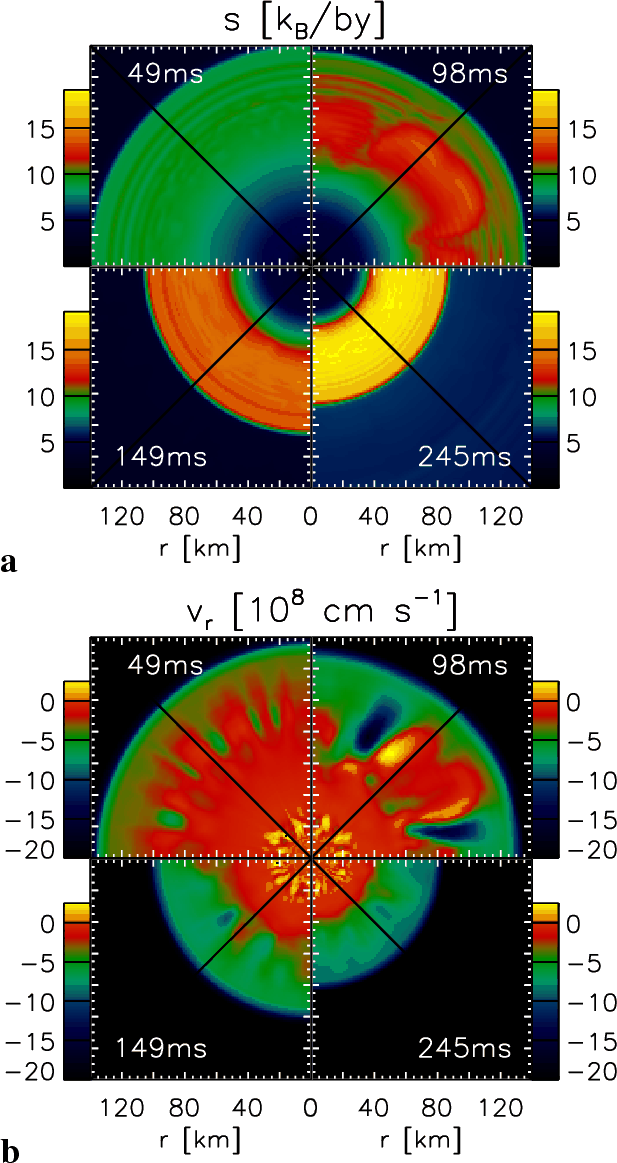$\begin{figure} \begin{tabular}{l} \put(0.9,0.3){{\Large\bf a}} \resizebox{8.8... ...izebox{8.8cm}{!}{\includegraphics{4654f28b.eps}} % \end{tabular}\par\end{figure}$ Figure 18: Postshock convection in Model s15_32. Panel a) shows snapshots of the entropy (in $k_{\rm B}$ /by) at four post-bounce times. Panel b) shows the radial velocity at the same times (the color bar is in units of 1000 km s^-1 and its upper end corresponds to 2500 km s^-1). The equatorial plane of the polar grid is marked by the black diagonal lines.
Open with DEXTER

In the text

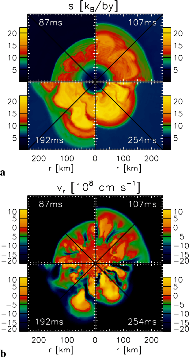$\begin{figure} \begin{tabular}{l} \put(0.9,0.3){{\Large\bf a}} \resizebox{8.8... ...izebox{8.8cm}{!}{\includegraphics{4654f29b.eps}} % \end{tabular}\par\end{figure}$ Figure 19: Postshock convection in Model s112_64. Panel a) shows snapshots of the entropy (in $k_{\rm B}$ /by) at four post-bounce times. Panel b) shows the radial velocity (in 1000 km s^-1) at the same times, with maximum values of up to 35 000 km s^-1 (bright yellow). The equatorial plane of the polar grid is marked by the diagonal lines.
Open with DEXTER

In the text

$\begin{figure} \par\includegraphics[width=8.4cm,clip]{4654f300.eps} \end{figure}$ Figure 20: Mass in the gain layer with the local specific binding energy as defined in Eq. (3) (but normalized per nucleon instead of per unit of mass) above certain values. The results are shown for Models s112_32 and s112_64 for times later than 100 ms after core bounce.
Open with DEXTER

In the text

$\begin{figure} \par\begin{tabular}{lr} \put(0.9,0.3){{\Large\bf a}} \includegr... ...f}} \includegraphics[width=8.2cm]{4654f31f.eps} % \end{tabular}\par\end{figure}$ Figure 21: Postshock convection in Model s112_128_f. Panels a)-c) show snapshots of the entropy for six post-bounce times. Panels d)-f) display the radial velocity at the same times with maximum values of up to 47 000 km s^-1 (bright yellow). In Panel d) also the convective activity below the neutrinosphere (at radii $r \protect\la 30~$ km) is visible. It is characterized by small cells, which are very similar to those observed in all other 2D models, too. The polar axis of the spherical coordinate grid is directed horizontally, the "north pole'' is on the right side.
Open with DEXTER

In the text

$\begin{figure} \par\includegraphics[width=8.4cm,clip]{4654f320.eps} \end{figure}$ Figure 22: Shock radii at the poles and at the equator versus post-bounce time for Model s112_128_f.
Open with DEXTER

In the text

$\begin{figure} \par\includegraphics[width=8.4cm,clip]{4654f330.eps} \end{figure}$ Figure 23: Kinetic energy, as a function of post-bounce time, associated with the lateral velocities of the matter between gain radius and shock (solid) and between the $\nu _{{\rm e}}$ sphere and shock (dashed) for Models s112_64 and s112_128_f. The rapid increase in case of Model s112_64 at $t_{\rm pb}\protect\ga 180$ ms is a numerical effect associated with lateral fluid flows which are enabled by our use of periodic boundary conditions at the angular grid boundaries.
Open with DEXTER

In the text

$\begin{figure} \par\includegraphics[width=8.4cm,clip]{4654f340.eps} \end{figure}$ Figure 24: The upper panel displays the "explosion energy'' of Model s112_128_f, defined by the volume integral of the "local specific binding energy'' $\varepsilon _{\rm bind}^{\rm shell}$ as given in Eq. (3), integrated over all zones where this energy is positive, i.e. $E_{\rm expl} = \int(\varepsilon_{\rm bind}^{\rm shell} > 0) \rho {\rm d}V~$ . The lower panel gives the mass in the gain layer with the local specific binding energy (per nucleon) above certain values. The evolution of these quantities as functions of post-bounce time is shown. Note the difference from Fig. 20.
Open with DEXTER

In the text

$\begin{figure} \par\begin{tabular}{cc} \put(0.9,0.3){{\Large\bf a}} \includegr... ...bf b}} \includegraphics[width=8.5cm]{4654f35b.eps} % \end{tabular} \end{figure}$ Figure 25: Radial profiles of the specific angular momentum j_z, angular velocity $\Omega$ , and ratio of centrifugal to gravitational force, $F_{\rm cent}/F_{\rm grav}$ , in the equatorial plane versus a) radius and b) mass for Model s15_64_r at different times. Note that the "enclosed mass'' in multi-dimensional simulations is defined here as the mass within a spherical volume of specified radius. Quantities plotted versus enclosed mass therefore do not represent Lagrangian information. Time is normalized to bounce. Note that in the upper right panel the lines for times -175 ms, 0, and 10 ms lie on top of each other because of specific angular momentum conservation and negligibly small rotational deformation of the collapsing stellar core until later after bounce.
Open with DEXTER

In the text

$\begin{figure} \par\begin{tabular}{lr} \put(0.9,0.3){{\Large\bf a}} \includegr... ... f}} \includegraphics[width=8.cm]{4654f36f.eps} % \end{tabular}\par\end{figure}$ Figure 26: Snapshots of Model s15_64_r. The rotation axis is oriented vertically. Panels a), b) show the distributions of the specific angular momentum j_z, of the angular frequency $\Omega$ , and of the ratio of centrifugal to gravitational force for the moment of bounce and for a post-bounce time of 271.1 ms, respectively. Note the different scales which represent enclosed mass M (which corresponds to values of mass enclosed by spheres of chosen radii) and radius r. The black lines mark the shock. Panels c), d) depict quantities which are of interest for discussing the physics in the gain layer at the time of maximum shock expansion and at the end of the simulation, respectively. The thick black line marks the shock, the thin black lines indicate the gain radius and $\nu _{{\rm e}}$ sphere. Panels e), f) provide analogous information inside the PNS at the onset of convection and at the end of the simulation, respectively. Instead of the gas entropy and ${Y_{\rm e}}$ , the total entropy including neutrino contributions and the total lepton number are plotted. The three black lines in panel f indicate from outside inward the neutrinospheres of $\nu _{{\rm e}}$ , $\bar\nu_{{\rm e}}$ , and $\nu _\mu$ .
Open with DEXTER

In the text

$\begin{figure} \par\includegraphics[width=8.4cm,clip]{4654f370.eps} \end{figure}$ Figure 27: Ratio of rotational energy to the gravitational energy, $\beta _{\rm rot}$ , as a function of time for Model s15_64_r. The quantity is shown for the whole computational volume (solid line) and for spherical volumes with an enclosed mass of the Fe-Si core (1.43 $\ensuremath {M_{\odot }}$ , dashed line) and of the Fe core (1.28 $\ensuremath {M_{\odot }}$ , dotted line), respectively. Note that in the latter two cases the time evolution of $\beta _{\rm rot}$ does not provide Lagrangian information, because matter is redistributed by rotational deformation and by convection.
Open with DEXTER

In the text

$\begin{figure} \par\includegraphics[width=8.4cm,clip]{4654f380.eps} \end{figure}$ Figure 28: ${Y_{\rm lep}}$ profile at 200 ms post-bounce time for a 1D model, a 2D model, and our 2D model with rotation. The plot shows angle-averaged quantities for the 2D cases.
Open with DEXTER

In the text

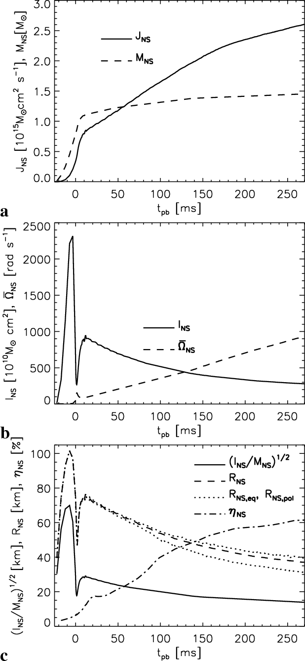$\begin{figure} \begin{tabular}{c} \put(0.9,0.3){{\Large\bf a}} \resizebox{8.8c... ...zebox{8.8cm}{!}{\includegraphics{4654f39c.eps}}\\ \end{tabular}\par\end{figure}$ Figure 29: a) Mass $M_{\rm NS}$ and total angular momentum $J_{\rm NS}$ of the "neutron star'' (defined by the matter with density above $10^{11}~\ensuremath{{\rm g}~{\rm cm}^{-3}}$ ) in Model s15_64_r. b) Moment of inertia $I_{\rm NS}$ and average angular frequency $\overline {\Omega }_{\rm NS} = I_{\rm NS}/J_{\rm NS}$ of the neutron star in Model s15_64_r. c) Average radius $R_{\rm NS}$ of the neutron star, defined as the radius of a sphere with the same volume as the deformed rotating neutron star, "effective'' radius defined as $R_{\rm eff,NS} = \sqrt {I_{\rm NS}/M_{\rm NS}}$ , and neutron star radii at the pole ( $R_{\rm NS,pol}$ ) and equator ( $R_{\rm NS,eq}$ ), for Model s15_64_r. Also shown is the eccentricity $\eta _{\rm NS} \equiv \sqrt {1-R_{\rm NS,pol}^2 / R_{\rm NS,eq}^2}$ .
Open with DEXTER

In the text

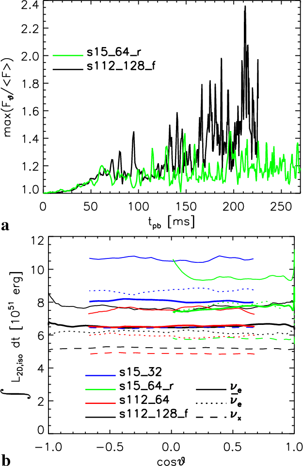$\begin{figure} \begin{tabular}{c} \put(0.9,0.3){{\Large\bf a}} \resizebox{8.8c... ...sizebox{8.8cm}{!}{\includegraphics{4654f40b.eps}}\\ % \end{tabular} \end{figure}$ Figure 30: a) Lateral maxima of the $\nu _{{\rm e}}$ flux relative to the average $\nu _{{\rm e}}$ flux versus time for Models s15_64_r and s112_128_f, evaluated at 400 km radius for an observer at rest. b) Time integral of the "isotropic equivalent luminosity'' $L_{\rm iso}$ - calculated by assuming that the flux in one polar direction is representative for all other directions - versus $\cos\vartheta$ for different models and neutrinos. The integral was performed from 10 ms to 200 ms after bounce; $\cos\vartheta=\pm1$ correspond to the poles, $\cos\vartheta=0$ to the equator. The thin lines are for an evaluation at 400 km radius for an observer at rest, the thick lines are given only for $\nu _{{\rm e}}$ and show the result at the $\nu _{{\rm e}}$ -sphere for an observer at rest.
Open with DEXTER

In the text

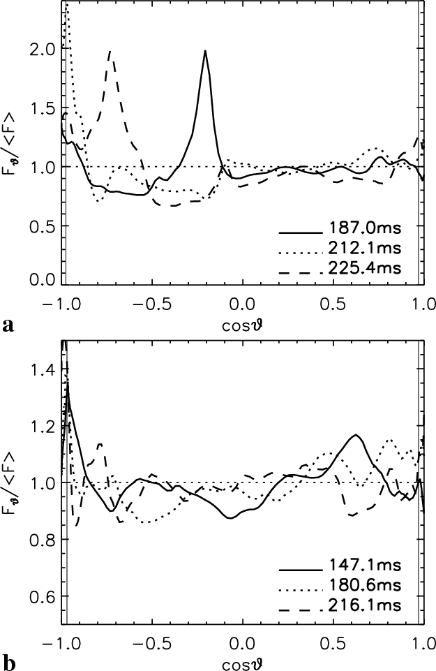$\begin{figure} \begin{tabular}{c} \put(0.9,0.3){{\Large\bf a}} \resizebox{8.8c... ...resizebox{8.8cm}{!}{\includegraphics{4654f41b.eps}} % \end{tabular} \end{figure}$ Figure 31: a) Ratio of electron neutrino flux to average flux (for an observer at rest at 400 km) versus cosine of the polar angle for Model s112_128_f for different post-bounce times. The times are picked such that large maxima of the flux ratio occur (see Fig. 30a). b) Same as panel a, but at the $\nu _{{\rm e}}$ sphere. The vertical solid lines mark the lateral boundaries of the region where the results were evaluated for Fig. 30a. Higher and lower latitudes were excluded because of possible artifacts from the reflecting boundaries.
Open with DEXTER

In the text

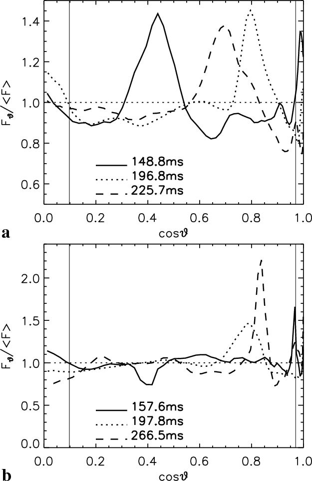$\begin{figure} \begin{tabular}{c} \put(0.9,0.3){{\Large\bf a}} \resizebox{8.8c... ...resizebox{8.8cm}{!}{\includegraphics{4654f42b.eps}} % \end{tabular} \end{figure}$ Figure 32: Same as Fig. 31, but for Model s15_64_r. The pole of the rotating model corresponds to $\cos\vartheta = 1$ .
Open with DEXTER

In the text

$\begin{figure} \includegraphics[width=12cm,clip]{4654f010.eps} \end{figure}$ Figure A.1: The progenitor data for temperature T, electron fraction ${Y_{\rm e}}$ , density $\rho$ , and the mass fractions of Si and O, $X_{\rm Si}$ and $X_{\rm O}$ , respectively, as provided to us by the stellar evolution modelers (see Table A.1 for references). The binding energy and entropy were derived with the EoS used in our simulations.

In the text

$\begin{figure} \includegraphics[width=12cm,clip]{4654f020.eps} \end{figure}$ Figure A.2: Radial profiles of the models during core collapse when the central density is $\rho_{\rm c} = 10^{11}~\ensuremath{{\rm g}~{\rm cm}^{-3}}$ .

In the text

$\begin{figure} \includegraphics[width=12cm,clip]{4654f030.eps} \end{figure}$ Figure A.3: Profiles as functions of enclosed mass of the models during core collapse when the central density is $\rho_{\rm c} = 10^{11}~\ensuremath{{\rm g}~{\rm cm}^{-3}}$ . The data are only shown for the stellar mass range that was included in the simulations. It corresponds to $r \leq 10~000$ km.

In the text

$\begin{figure} \par\includegraphics[width=8.4cm,clip]{4654f040.eps} \end{figure}$ Figure B.1: Central density versus time remaining until core bounce for all 1D models.

In the text

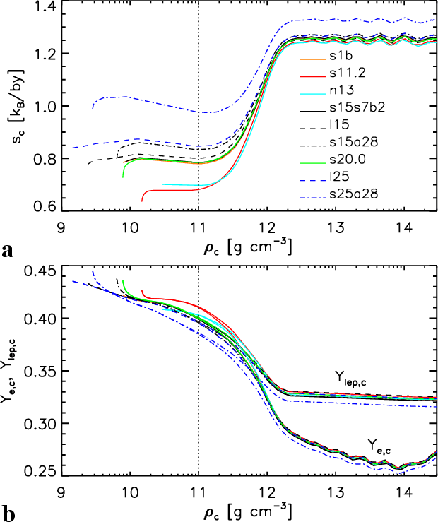$\begin{figure} \begin{tabular}{l} \put(0.9,0.3){{\Large\bf a}} \resizebox{8.8... ...\resizebox{8.8cm}{!}{\includegraphics{4654f05b.eps}} \end{tabular} \end{figure}$ Figure B.2: Central entropy (panel a)) and central electron and lepton fraction (panel b)) versus central density during core collapse for all 1D models. The vertical dotted line marks the time of comparison at a central density $10^{11}~\ensuremath{{\rm g}~{\rm cm}^{-3}}$ in Figs. A.2 and A.3.

In the text

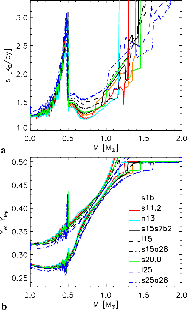$\begin{figure} \begin{tabular}{l} \put(0.9,0.3){{\Large\bf a}} \resizebox{8.8... ...resizebox{8.8cm}{!}{\includegraphics{4654f06b.eps}} % \end{tabular} \end{figure}$ Figure B.3: Entropy (panel a)) and electron and lepton fraction (panel b)) versus enclosed mass at the time of shock formation.

In the text

$\begin{figure} \par\includegraphics[width=16cm,clip]{4654f070.eps} \end{figure}$ Figure B.4: Post-bounce evolution of the models in spherical symmetry. The left panels show phases around the core bounce with the last stage of infall (t < 0), prompt shock propagation, neutrino burst, and early accretion phase of the shock. The right panels depict the post-bounce accretion phase of the stalled shock. From top to bottom, the panels display the shock radius, the mass accretion rate through the shock, the mass enclosed by the shock ( left) or PNS baryonic mass ( right), the PNS radius, and the electron neutrino ( left) or total neutrino ( right) luminosity at r=400 km for an observer at rest. The PNS mass and radius are defined by the corresponding values at the $\nu _{{\rm e}}$ sphere.

In the text

$\begin{figure} \par\includegraphics[width=8.4cm,clip]{4654f100.eps} \end{figure}$ Figure B.5: Integrated lepton number ( top) and energy loss of the 1D models versus time.

In the text

$\begin{figure} \includegraphics[width=12cm]{4654fa10.eps} \end{figure}$ Figure C.1: Results of a linear analysis of the structural changes of the PNS in response to the removal of lepton number or energy, respectively, at different densities and thus enclosed masses $M_{\rm p}$ . The lower lines correspond to the expansion when one electron is removed, while the upper lines depict the contraction when an energy of $10~\ensuremath{{\rm MeV}}$ is extracted. The lines correspond to post-bounce times of 73 ms (solid) and 240 ms (dashed). The labels "dump'' and "drain'' denote the density windows between the vertical, dotted lines, which roughly indicate where PNS convection deposits or extracts, respectively, lepton number and energy.

In the text

$\begin{figure} \begin{tabular}{c} \put(0.9,0.3){{\Large\bf a}} \includegraphic... ...b}} \includegraphics[width=8.5cm]{4654fa2b.eps} % \end{tabular}\par\end{figure}$ Figure D.1: Panel a) depicts the ${Y_{\rm lep}}$ profiles for three times around the onset of PNS convection, comparing a 1D model (s15s7b2), a 2D model (s15_32, for which angular-averaged values are plotted), and a 1D model with PNS mixing scheme (s15_mix). Panel b) shows ${Y_{\rm lep}}$ , the total entropy $s+s_\nu$ , the radial velocity v_r, and the Brunt-Väisälä-frequency $\omega _{\rm BV}$ (clockwise from top left to bottom left) in the PNS convective region for Model s15_32 shortly after the onset of PNS convection.

In the text

$\begin{figure} \par\includegraphics[width=8.5cm,clip]{4654f120.eps} \end{figure}$ Figure E.1: Maximum fluctuations of the density within the core of $1.5~\ensuremath{M_{\odot}}$ at four times during the collapse of Model s15_64_p ( top). The initially imposed random perturbations are damped strongly during the subsonic collapse in the inner part of the Fe core. The corresponding density and velocity profiles (averaged in latitude) are shown in the middle and bottom panels, respectively. The short solid lines cutting the profiles in the bottom plot indicate the position of the sonic point.

In the text

$\begin{figure} \par\includegraphics[width=8.4cm,clip]{4654f12b.eps} \end{figure}$ Figure E.2: Standard deviations of the density fluctuations in lateral direction, $\sigma _\rho$ , as defined in Buras et al. (2006, Eq. (24)) for different mass shells versus the (time-dependent) radius r_M of these mass shells. The dashed lines represent fits according to $\sigma _\rho \propto r_M^{-1/2}$ , the thick black bars mark the phases of the collapse when the infall velocity of a mass shell is more than 60% of the local sound speed, and the white bars mark the phases when the local infall velocity is supersonic.

In the text

$\begin{figure} \par\includegraphics[width=7.8cm,clip]{4654f080.eps} \end{figure}$	Figure 1: The advection timescales as defined in Eq. (1) versus post-bounce time. The lines are smoothed over time intervals of 5 ms.
Open with DEXTER

$\begin{figure} \par\includegraphics[width=7.8cm,clip]{4654f090.eps} \end{figure}$	Figure 2: The timescale ratios, $\tau _{\rm adv} / \tau _{\rm heat}$ , as functions of time. The lines are smoothed over time intervals of 5 ms.
Open with DEXTER

$\begin{figure} \par\includegraphics[width=8cm,clip]{4654f150.eps} \end{figure}$	Figure 6: Brunt-Väisälä frequency (Eq. (5)), using Eq. (7) as stability criterion, evaluated for different 1D models at 20, 30, and 40 ms after bounce.
Open with DEXTER

$\begin{figure} \par\includegraphics[width=8cm,clip]{4654f170.eps} \end{figure}$	Figure 7: Lepton number and total entropy versus enclosed mass in the PNS for the 1D model s15s7b2 for different post-bounce times before the onset of PNS convection in the corresponding 2D simulation.
Open with DEXTER

$\begin{figure} \par\includegraphics[width=8.5cm,clip]{4654f190.eps} \end{figure}$	Figure 10: Lepton number, total entropy, specific internal energy, and density profiles versus enclosed mass in the PNS for a sample of 1D (dotted) and 2D simulations of different progenitor stars, 200 ms after bounce (i.e., approximately 160 ms after the onset of PNS convection). For the 2D models angle-averaged quantities are plotted.
Open with DEXTER

$\begin{figure} \par\includegraphics[width=8.4cm,clip]{4654f200.eps} \end{figure}$	Figure 11: Radius of the electron neutrinosphere (as a measure of the PNS radius) for the 2D models and their corresponding 1D models. For Model s15_64_r we show the equatorial ( upper) and polar ( lower) neutrinospheric radii. For other 2D models, angle-averaged quantities are plotted.
Open with DEXTER

$\begin{figure} \par\includegraphics[width=8.6cm,clip]{4654f230.eps} \end{figure}$	Figure 14: Differences between the total lepton number ( top) and energy losses ( bottom) of the 2D models and their corresponding 1D models as functions of post-bounce time. Here, $\cal {L}$ is the total lepton number flux, and L is the total neutrino luminosity.
Open with DEXTER

$\begin{figure} \par\includegraphics[width=8.4cm,clip]{4654f250.eps} \end{figure}$	Figure 15: Maximum and minimum shock radii as functions of time for the 2D models of Table 1, compared to the shock radii of the corresponding 1D models (dotted lines).
Open with DEXTER

$\begin{figure} \par\includegraphics[width=8.4cm,clip]{4654f260.eps} \end{figure}$	Figure 16: Minimum and maximum gain radii as functions of post-bounce time for our $15~\ensuremath{M_{\odot}}$ 2D simulations compared to the gain radius of the corresponding 1D models.
Open with DEXTER

$\begin{figure} \begin{tabular}{l} \put(0.9,0.3){{\Large\bf a}} \resizebox{8.8... ...izebox{8.8cm}{!}{\includegraphics{4654f28b.eps}} % \end{tabular}\par\end{figure}$	Figure 18: Postshock convection in Model s15_32. Panel a) shows snapshots of the entropy (in $k_{\rm B}$ /by) at four post-bounce times. Panel b) shows the radial velocity at the same times (the color bar is in units of 1000 km s^-1 and its upper end corresponds to 2500 km s^-1). The equatorial plane of the polar grid is marked by the black diagonal lines.
Open with DEXTER

$\begin{figure} \begin{tabular}{l} \put(0.9,0.3){{\Large\bf a}} \resizebox{8.8... ...izebox{8.8cm}{!}{\includegraphics{4654f29b.eps}} % \end{tabular}\par\end{figure}$	Figure 19: Postshock convection in Model s112_64. Panel a) shows snapshots of the entropy (in $k_{\rm B}$ /by) at four post-bounce times. Panel b) shows the radial velocity (in 1000 km s^-1) at the same times, with maximum values of up to 35 000 km s^-1 (bright yellow). The equatorial plane of the polar grid is marked by the diagonal lines.
Open with DEXTER

$\begin{figure} \par\includegraphics[width=8.4cm,clip]{4654f300.eps} \end{figure}$	Figure 20: Mass in the gain layer with the local specific binding energy as defined in Eq. (3) (but normalized per nucleon instead of per unit of mass) above certain values. The results are shown for Models s112_32 and s112_64 for times later than 100 ms after core bounce.
Open with DEXTER

$\begin{figure} \par\includegraphics[width=8.4cm,clip]{4654f320.eps} \end{figure}$	Figure 22: Shock radii at the poles and at the equator versus post-bounce time for Model s112_128_f.
Open with DEXTER

$\begin{figure} \par\includegraphics[width=8.4cm,clip]{4654f380.eps} \end{figure}$	Figure 28: ${Y_{\rm lep}}$ profile at 200 ms post-bounce time for a 1D model, a 2D model, and our 2D model with rotation. The plot shows angle-averaged quantities for the 2D cases.
Open with DEXTER

$\begin{figure} \begin{tabular}{c} \put(0.9,0.3){{\Large\bf a}} \resizebox{8.8c... ...resizebox{8.8cm}{!}{\includegraphics{4654f42b.eps}} % \end{tabular} \end{figure}$	Figure 32: Same as Fig. 31, but for Model s15_64_r. The pole of the rotating model corresponds to $\cos\vartheta = 1$ .
Open with DEXTER