A&A 456, 827-838 (2006)
DOI: 10.1051/0004-6361:20054794

Shears from shapelets

K. Kuijken¹

Leiden Observatory, PO Box 9513, 2300 RA Leiden, The Netherlands

Received 31 December 2005 / Accepted 15 June 2006

Abstract
Aims. Accurate measurement of gravitational shear from images of distant galaxies is one of the most direct ways of studying the distribution of mass in the universe. We describe a new implementation of a technique for measuring shear that is based on the shapelets formalism.
Methods. The shapelets technique describes PSF and observed images in terms of Gauss-Hermite expansions (Gaussians times polynomials). It allows the various operations that a galaxy image undergoes before being registered in a camera (gravitational shear, PSF convolution, pixelation) to be modeled in a single formalism, so that intrinsic ellipticities can be derived in a single modeling step.
Results. The resulting algorithm, and tests of it on idealized data as well as more realistic simulated images from the STEP project, are described. Results are very promising, with attained calibration accuracy better than four percent (1 percent for round PSFs) and PSF ellipticity correction better than a factor of 20. Residual calibration problems are discussed.

Key words: gravitational lensing - techniques: image processing - cosmology: dark matter

1 Introduction

Weak gravitational lensing is recognized as a profitable way to study the dark matter distribution in the universe, and with a series of ever wider-field astronomical cameras coming online, very large weak lensing surveys are being planned and performed. The inevitable source of noise in weak lensing measurements is shape noise, caused by the diversity of projected galaxy shapes on the sky. To beat down the noise, very large numbers of galaxy ellipticities need to be averaged: thus new lensing surveys such as the CFHT Legacy Survey (Hoekstra et al. 2005), the CTIO survey (Jarvis et al. 2003), the VIRMOS-Descart survey (van Waerbeke et al. 2005) or the recently-approved Kilo-Degree Survey (KIDS) on the VLT Survey Telescope, will contain millions of background sources, which in principle should enable very accurate shear measurements.

This averaging down of the shape noise through large number statistics only makes sense if systematic errors can be controlled: the main one is still the blurring of the source images by atmosphere, telescope and detector pixels. The commonly-used Kaiser et al. (1995; henceforth KSB) and Luppino & Kaiser (1997) methods provide recipes for correcting these effects, and are very successful. Nevertheless, they are based on an idealized model of the effect of point spread function (PSF) convolution on ellipticity, and it is possible to construct plausible PSFs that it fails to correct properly (e.g., Hoekstra et al. 1998, Appendix D). Therefore it seems unlikely that the KSB recipes will deliver the factor of 10 to 100 improvement in fidelity that will be required to exploit the new surveys (Erben et al. 2001).

A number of different approaches have been put forward to improve PSF correction (Kuijken 1999; Kaiser 2000; Rhodes et al. 2000; Bernstein & Jarvis 2002; Refregier & Bacon 2003; Mandelbaum et al. 2005). In this paper we present a new technique which combines elements from most of these.

The paper is organized as follows: in Sect. 2 shear and ellipticity are defined, and the effect of one on the other. Section 3 summarizes the shapelets formalism, and describes how a shapelet description of a source and its PSF can be used to generate an ellipticity estimate that is useful for shear estimation. Section 4 substantiates the approach with idealized tests of the algorithm. In Sect. 5 a software pipeline is presented that implements the full processing chain from an astronomical image to a shear estimate. Results of applying the pipeline to test data from the STEP project are shown in Sect. 6. In Sect. 7 we compare with other techniques, and Sect. 8 gives the conclusions.

   
2 Preliminaries

2.1 Shear and distortion

Following the usual practice, we parameterize the effect of weak gravitational lensing on a distant source in terms of a shear $(\gamma_1,\gamma_2)$ and a convergence $\kappa$: the distorted image $I_{\rm lensed}(x,y)$ is derived from the original I(x,y) via the transformation $I_{\rm lensed}(x,y) = I(x',y')$, where

 

$$\left(\!\!\begin{array}{c}x'\\ y'\end{array}\!\!\right) \left(\begin{array}{cc} 1-\gamma_1-\kappa&-\gamma_2\\ -\gamma_2&... ...\kappa\end{array}\right) \left(\!\!\begin{array}{c}x\\ y\end{array}\!\!\right)$$ =

$$\equiv (1-\kappa) \left(\begin{array}{cc} 1-g_1&-g_2\\ -g_2&1+g_1\end{array}\right) \left(\!\!\begin{array}{c}x\\ y\end{array}\!\!\right)\cdot$$ (1)

The first matrix in this equation (the distortion matrix) represents the transformation from observed (x,y) to undistorted (x',y') coordinates.

Without knowledge of the intrinsic source size, only the distortion $(g_1,g_2)\equiv(\gamma_1,\gamma_2)/(1-\kappa)$, which affects the shape of the source, can be measured (Schneider & Seitz 1995).

2.2 Ellipticity

We define the ellipticity of an object's image I as follows:

Let $I_{\rm ell}$ be the model image with constant-ellipticity isophotes that best approximates I. Then the ellipticity (e₁,e₂) of I is defined such that a distortion of (-e₁,-e₂) makes $I_{\rm ell}$ circular.

The major axis position angle $\phi$ and the axis ratio q of an elliptical source are simply related to (e₁,e₂):

$$q={1-e\over 1+e}\qquad\hbox{and}\qquad e_1=e\cos2\phi,\qquad e_2=e\sin2\phi.$$ (2)

This definition is similar to the one adopted by Bernstein & Jarvis (2002; henceforth BJ02), but does not explicitly force a fit to an elliptical Gaussian.

As discussed by BJ02, expressing the shapes of objects in terms of distortions e has a practical advantage: in this formulation it is simple to calculate the response of object shapes to small distortions. An elliptical source with ellipticity (e₁,e₂) that is sheared by a small amount (g₁,g₂) can be viewed as a circular source that is sheared twice, first by e_i and then by g_i, giving a combined distortion matrix

$$\left(\begin{array}{cc} 1-e_1&-e_2\\ -e_2&1+e_1\end{array}\right... ...e_2-g_2-e_1g_2+e_2g_1 & 1+e_1+g_1+e_1g_1+e_2g_2\\ \end{array}\right)\cdot\quad$$ (3)

This matrix is no longer a pure distortion matrix (which would have to be symmetric and of trace 2), but some algebra shows that this matrix can be decomposed into a magnification, a rotation and a distortion:

$$\left(\begin{array}{cc} 1-e_1&-e_2\\ -e_2&1+e_1\end{array}\right... ...1-e_1-\delta_1&-e_2-\delta_2\\ -e_2-\delta_2&1+e_1+\delta_1\end{array}\right),$$ (4)

where, to first order in the distortion g_i,

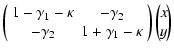
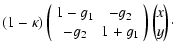
K=e₁g₁+e₂g₂ (5)

R=e₁g₂-e₂g₁ (6)

$$\delta_1=(1-e_1^2-e_2^2)g_1$$ (7)

$$\delta_2=(1-e_1^2-e_2^2)g_2.$$ (8)

Thus the action of a small distortion g on an elliptical source with ellipticity e_i (according to the definition in Eq. (1)) is equivalent to acting on a circular source with, successively, a magnification, a rotation (neither of which affect the shape of a circular source), and a distortion by $e_i+\delta_i$.

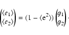
Assuming now that we have an ensemble of elliptical sources, of random orientations, so that before distortion $\langle e_i\rangle=0$ and $\langle e_1^2\rangle+\langle e_2^2\rangle\equiv \langle {\rm e}^2\rangle$, the average ellipticity of the population after a distortion (g₁,g₂) is simply

$$\left(\!\! \begin{array}{c}\langle e_1\rangle\\ \langle e_2\r... ...left(\!\! \begin{array}{c}g_1\\ g_2\end{array}\!\!\right)\cdot$$ (9)

3 Shapelets

The shapelets basis is described in Refregier (2003). It consists of the two-dimensional Cartesian Gauss-Hermite functions, famous as the energy eigenstates of the 2D quantum harmonic oscillator:

$$B^{ab}(x,y)=k^{ab}\beta^{-1} {\rm e}^{-[(x-x_{\rm c})^2+(y-y_{\rm c})^2]/2\beta^2} H^a(x/\beta) H^b(y/\beta).$$ (10)

Here (x,y) are coordinates on the image plane, $x_{\rm c}$ and $y_{\rm c}$ are the center of the expansion, B^ab is the basis function of order (a,b), H^a is the Hermite polynomial of order a and $\beta$ is a scale radius. k^ab is a normalization constant chosen so that $\left(B^{ab}\right)^2$ integrates to one.

Shapelets are a convenient basis set for describing astronomical images because of the compact way in which various operators (translation, magnification, rotation, shear) can be expressed as matrices that act on the shapelet coefficients. Shapelets have a free scale radius $\beta$ (the size of the Gaussian core of the functions), and R03 shows how the coefficients transform under change of $\beta$, and how to convolve objects with different scale radii.

To avoid introducing a preferred direction, the expansion should be truncated in combined order N=a+b, not in a or b separately. (A basis set truncated in N is complete under rotation. Effectively, such a truncation describes an image as a product of a circular Gaussian with an inhomogeneous polynomial in x and y of order N. Rotation of such an image will mix the xⁱy^j terms at constant i+j.)

The reason for choosing shapelets as a formalism for weak lensing analysis is its ability to describe the main operations that a galaxy image undergoes before it is registered at a telescope focal plane: in reverse order, pixelation, convolution with a PSF, and distortion.

In this paper we concentrate on well-sampled (PSF FWHM at least 3-4 pixels), ground-based seeing-limited images. It remains to be seen to what extent diffraction-limited PSFs, and undersampling, can be handled with this formalism.

3.1 Pixelation

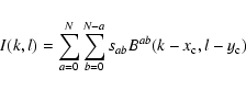
An image that is registered on a CCD is pixelated: the flux on the surface of the detector is read out in binned form. Mathematically, the flux is first boxcar smoothed (i.e., convolved with a pixel), and then sampled at a spatial frequency of once per pixel. Therefore, if we fit a shapelet expansion to the binned image I(k,l) as a linear superposition of the basis functions B^ab:

$$I(k,l)=\sum_{a=0}^N\sum_{b=0}^{N-a} s_{ab} B^{ab}(k-x_{\rm c},l-y_{\rm c})$$ (11)

then the shapelet coefficients s_ab describe the pixel-convolved image directly. If a similar fit is made to a PSF image that is pixelated in the same way, then the intrinsic, pre-seeing image is exactly the deconvolution of the two shapelet expansions (apart from the effects of noise, undersampling, and truncation of the shapelet expansions).

3.2 PSF convolution

Convolution with the PSF can be expressed as multiplication with a PSF matrix ${\bf P}_{a_1b_1a_2b_2}(\beta_{\rm in},\beta_{\rm out})$: if the shapelet coefficients of the PSF are p_ab, and those of a model source are m_ab, then their convolution is

$$\left(\sum_{a,b} p_{ab}B^{ab}_{\beta_{\rm psf}}\right) \otimes \l... ...beta_{\rm in},\beta_{\rm out})m_{a_2b_2} \right) B^{a_1b_1}_{\beta_{\rm out}} .$$ (12)

The subscripts on B^ab identify the scale radius $\beta$, which can be different for the three shapelet series involved: those for the PSF, input model source and output result of the convolution. ${\bf P}(\beta_{\rm in},\beta_{\rm out})$ convolves a shapelet expansion with scale radius $\beta_{\rm in}$ with the PSF, resulting in a shapelet expansion with scale radius $\beta_{\rm out}$. The coefficients of the PSF matrix are

$${\bf P}_{a_1b_1a_2b_2}(\beta_{\rm in},\beta_{\rm out})= \sum_... ...3}^{\beta_{\rm out}\beta_{\rm in}\beta_{\rm psf}} p_{a_3b_3}.$$ (13)

Here the elemental convolution matrix $C_{nml}^{\beta_3\beta_1\beta_2}$ expresses the convolution of two one-dimensional shapelets of scales $\beta_1$ and $\beta_2$ as a new shapelet series with scale $\beta_3$. A recurrence relation for C_nml is given in R03.

   
3.3 Ellipticity from shapelets

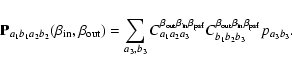
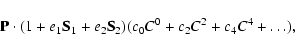
Given a PSF and a PSF-convolved source, both expressed as shapelet series, we determine the ellipticity of the source by modeling it as a PSF-convolved, distorted circular source of arbitrary radial brightness profile. This approach is similar to the one described in Kuijken (1999), but it is more effective when expressed in terms of shapelets.

A circular source of arbitrary radial brightness profile can be written as a series of circular shapelets Cⁿ of the form $c_0C^0+c_2C^2+c_4C^4+\ldots$, where the c_n are free coefficients. The Cⁿ (see Appendix) are normalized to have unit integral over x,y, so c_n gives the total counts in each component. After distortion of such a source, it becomes an elliptical source which, to leading order in ellipticity e, can be written as

$$(1+e_1{\bf S}_1+e_2{\bf S}_2)(c_0C^0+c_2C^2+c_4C^4+\ldots)$$ (14)

where ${\bf S}_i$ are the first-order shear operators (see R03).

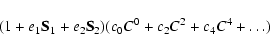
This machinery allows us to write the model for the observed source as

$${\bf P}\cdot(1+e_1{\bf S}_1+e_2{\bf S}_2)(c_0C^0+c_2C^2+c_4C^4+\ldots),$$ (15)

expressed as a set of shapelet coefficients that depend on the e_iand the c_n. Fitting this model to the shapelet coefficients of the observed source (with their errors) yields the best-fit ellipticity (e₁,e₂) and the associated errors.

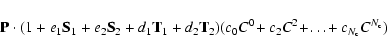
To improve the accuracy, we make two modifications: we add centroid error parameters, and we only fit the model to a subset of the shapelet expansions. The centroid error parameters are included to allow for a mismatch between the center of the object and its shapelet expansion. If the PSF and/or the galaxy have some lopsidedness to them, the center of their best-fit shapelet expansion may not be at the flux-weighted center of the source (since our centering technique simply requires the 01 and 10 components to be exactly zero). Hence the centroid may move under convolution, which would spoil the fit. To guard against this, instead of fitting Eq. (15) we fit a model of the form

$${\bf P}\cdot(1+e_1{\bf S}_1+e_2{\bf S}_2+d_1{\bf T}_1+d_2{\b... ...c_0C^0\!+c_2C^2\!+\!\ldots\!+c_{N_{\rm c}}C^{N_{\rm c}}) \ \ \$$ (16)

instead. The free translation terms $d_i{\bf T}_i$ in the model are expressed in terms of the shapelet operators ${\bf T}_i$.

The second modification is made to contain truncation errors. While the shapelet basis is complete, and hence can describe any source given enough terms, in practice the fact that the source is only sampled in a finite set of pixels means that the expansion needs to be truncated. Hence, except in very special cases, the PSF and galaxy are not described perfectly by a truncated shapelet series. The missing information propagates through the analysis, and is a source of systematic error in the PSF convolution (as some PSF terms may be missing) and in the calculation of the action of shear (since shearing high-order shapelets generates also lower-order terms).

Truncation effects can be seen most clearly if we re-express the shapelets in polar $(r,\theta)$ coordinates (they become Gaussians times Laguerre polynomials of r - see BJ02, R03, Massey & Refregier 2005). Polar shapelets are combinations of Cartesian shapelets B^ab of the same order N=a+b, whose angular dependence is a pure sine or cosine of $m\theta$, for angular order m. The order of the Laguerre polynomial is N, with $N\ge m$ and N+m even.

The translation and shear operators, when applied to a polar shapelet of order (N,m), generate terms at order $(N\pm1,m\pm1)$ and $(N\pm2,m\pm2)$, respectively. If we truncate the shapelet series of the best-fit circular model for the pre-seeing, pre-shear galaxy at order $N_{\rm c}$, then to be consistent the m=1 and m=2 series must be truncated at order $N_{\rm c}-1$ and $N_{\rm c}-2$, respectively.

Figure 1: The information used in the ellipticity determination, for shapelet expansion to order N=8. On the left, the Cartesian shapelet coefficients that are fitted to describe a source and its associated PSF. On the right, the same information has been rearranged into a polar shapelet expansion (the two may be transformed into one another by appropriate mixing of the terms at order $N\equiv a+b$). The heavy line indicates the polar shapelets from which the ellipticity is estimated by a fit to Eq. (16). Note the safety margin at order N-1 and N, and the fact that only azimuthal orders between -2 and +2 are fitted.

Open with DEXTER

Note that we are never completely safe from truncation effects: in particular, complex PSFs can in principle mix coefficients of all orders. The problem is minimized, but not completely eliminated, by adopting suitable scale radii so that the amount of information carried in the high-order coefficients is small. We further include a "safety margin'' by setting $N_{\rm c}=N-2$, in case the highest-order shapelet coefficients are affected by PSF structure at even higher order. The scheme is illustrated for the typical case of N=8 in Fig. 1. The highest-order polar shapelet coefficients that should be included in the fit are $(N_{\rm c},0)$, $(N_{\rm c}-1,\pm1)$ and $(N_{\rm c}-2,\pm2)$.

In summary, from the shapelet series for each source, up to Cartesian order $N_{\rm max}$, we form a truncated polar shapelet series including terms of order $(m=0, N=0,2,\ldots ,N_{\rm max}-2)$, $(m=1,N=1,3,\ldots ,N_{\rm max}-3)$ and $(m=2,N=2,4,\ldots, N_{\rm max}-4)$. The effect of the shear, translation and PSF operators on circular basis functions up to order $N_{\rm max}-2$is then calculated up to order $N_{\rm max}$, and the result likewise converted to polar shapelets up to order $N_{\rm max}-2$.

Least-squares fitting the model to each source yields an ellipticity estimate (e₁,e₂), expressed as the shear that needs to be applied to a circular source to fit the object optimally.

Performing the least-squares fit is straightforward to do numerically. $\chi^2$ is a fourth-order polynomial in the fit parameters $\{c_0,c_2,\ldots,c_{N-2},e_1,e_2,d_1,d_2\}$, and the minimum can typically be found in a few Levenberg-Marquardt iterations (Press et al. 1986).

The errors on the shapelet coefficients for each source can be derived from the photon noise, and these can be propagated through in the $\chi^2$ function. The second partial derivatives of $\chi^2$ at the best fit give the inverse covariance matrix, which can be inverted to show the variance and covariances between the fit parameters. This results in proper error estimates on all parameters, in particular on e₁ and e₂. In practice the errors on e_i are only weakly correlated with those on d_i and c_n.

4 Tests

 We now describe some elementary tests of this approach.

4.1 Test of ellipticity estimates

For small ellipticity e the linear shear operator provides a good description of the action of the shear, but for larger ehigher-order corrections come into play, and these corrections depend on the radial brightness profile. We have calibrated these corrections empirically using a set of model sources that follow a Sersic (1968) distribution of brightness, of index 1-4. Each source was sheared by varying amounts and encoded into shapelets using a range of different scale radii. The first-order ellipticity estimate $e_{\rm 1st}$ derived by fitting a model of Eq. (14) was then compared to the true ellipticity (see Fig. 2). For small e the correct ellipticity is recovered, but at larger e the discrepancy grows. Fitting the residuals versus the radial profile shape parameters c₀, c₂, c₄, it turns out that the true ellipticity $e_{\rm true}$ can be derived from the fitted 1st-order estimate by applying the correction factor

$${e_{\rm true}\over e_{\rm 1st}} \simeq 1-e_{\rm 1st}^2\left(-0.41+{0.085c_2+0.63 c_4\over c_0}\right)\cdot$$ (17)

The formula is valid to better than 1% accuracy for e<0.7, corresponding to axis ratios of nearly 6:1.

Figure 2: Empirical calibration of the post-linear correction to the measurement of e. Top left: fractional error on derived 1st-order ellipticity e for a range of different scale parameters and Sersic indices. Top right: fractional error of the corrected ellipticity. Bottom left: the coverage of the c2/c0, c4/c0plane by the models. The four groups of points correspond, from top to bottom, to Sersic index 4, 3, 2 and 1. The horizontal spread is mostly a consequence of using different scale radii $\beta$. Bottom Right: residuals on 1st-order ellipticity vs. the linear combination of c'/c0=(0.085c2+0.63c4)/c0 for input ellipticity 0.4, showing that this parameter drives the scatter.

Open with DEXTER

Below we will, in fact, NOT apply this correction, because the errors on c₀, c₂ and c₄ are typically so high, and (in the case of small, barely resolved sources) correlated, that the correction factor cannot be determined accurately. Fortunately most galaxies in the sky have ellipticity below 0.3, where the correction is below 3%. If necessary, the accuracy could be further increased by evaluating the effect of shear on the shapelet basis functions to higher order in Eq. (16).

   
4.2 Choice of scale radius

A truncated shapelet expansion can only describe deviations from a Gaussian over a particular range of spatial scales (which widens with order N). For ellipticity determinations the outer parts of galaxy and PSF images are most important (e.g., the classic second moments depend on the 3rd moment of the radial profile), so there is some advantage to taking as large a scale radius as possible. On the other hand, this radius should not be so large that the inner structure of the source cannot be resolved.

We have found that, for shapelet expansions up to order N=8 or higher, taking a scale radius which is 1.3 times the dispersion of the best-fit Gaussian works well for a range of model PSFs. Figure 3 shows an example for a Moffat PSF with index 2: both the core and the wings can be fitted adequately with this choice of $\beta$.

Figure 3: Different shapelet fits to a Moffat PSF $(1+\alpha r^2)^{-2}$ with FWHM of 12 pixels. Top panel: the solid line shows a cross-section of an 8th-order fit, using the dispersion of the best-fit Gaussian as scale radius. The dotted line shows the corresponding fit for a scale radius that is a factor of 1.3 times larger. The lower panel shows the PSF multiplied by radius3, in order to accentuate the residuals in the wings. Dots are the actual (monte-carlo realized) pixelated PSFs used in the simulations of Sect. 4. Note how the increased scale radius makes for a much better fit in the outer regions, without a serious degradation in the core of the PSF.

Open with DEXTER

The impact of the choice of scale radius on ellipticity measurements is shown in Fig. 4, for typical images. The factor 1.3 represents a good compromise, though its exact value is not critical.

Figure 4: Illustration of the effect of the choice of scale radius on the ellipticity measurement. Each curve shows, for a different galaxy profile, how the derived e depends on the choice of scale radius (expressed as a multiple of the dispersion of the best-fitting round Gaussian). Each model galaxy had an effective radius of 4 pixels and ellipticity 0.3, and was convolved with a PSF of Moffat index 2 and FWHM 8 pixels. The $\beta$ for convolved source and PSF are both scaled by the same factor.

Open with DEXTER

   
4.3 Test of PSF correction

Correcting for the effects of PSF convolution (dilution of ellipticity by a round PSF, or biasing of ellipticity by an elongated one) is the most critical part of weak lensing. The following tests show how well the shapelets technique can do this.

For the tests we generate simulated, high signal-to-noise (S/N) sources. To be sure that pixelation effects are taken into account properly, and that the PSF convolutions are done accurately, a brute-force technique is used: each source is built of individual "photons'' that are drawn from a 2D Sersic distribution, sheared if required, then have a "PSF'' displacement added to them, and finally are added to the pixel in which they fall. We use 10 million photons per source, which gives effectively noise-free images (S/N $\ga$ 1000).

We ran three sets of tests. In each case we explore galaxies with Sersic laws $f(r)\sim\exp~(-k r^{1/n_{\rm s}})$ with indices $n_{\rm s}=0.5$(Gaussian), 1 (exponential), 2, 3 and 4 (de Vaucouleur), and use PSFs with a Moffat profile $(1+\alpha r^2)^{-\beta_{\rm m}}$ of index $\beta_{\rm m}=2$, 3 and 9 (nearly Gaussian). All galaxies are scaled to an intrinsic effective radius of 4 pixels, and the PSF FWHM's range from 4 to 12 pixels. We use shapelet expansions to order N=8 and 12, and scale radii of 1.3 times the dispersion of the best-fit Gaussian.

First, to test the "shear calibration'' factor, we check how well we can recover the shear of a galaxy that is sheared by g₁=0.1 and convolved with a round PSF. Figure 5 shows the result: any calibration error is at the sub-percent level; the worst results are obtained for the most non-Gaussian PSFs ( $\beta_{\rm m}=2$). The noise in the curves suggests that we are also limited by the accuracy of the Monte-Carlo simulations of the galaxies, and by the numerics of the software implementation of the method.

The second test shows to what extent PSF ellipticity pollutes the shear estimate. The input PSFs were given an elipticity e₁=0.1(axis ratio 0.82), and convolved with round galaxies. The recovered e is shown in Fig. 6. The residual effect is at most half a percent (worst case), which represents a correction of the PSF ellipticity by a factor of better than 20. The best results are obtained for lowish Sersic indices (below 2) and for PSFs with not too extended wings (Moffat index 3 or higher). Perhaps surprisingly, the larger the PSF (for the same galaxy size) the better the correction: presumably this is a small sampling effect.

Finally, we introduced a lopsided PSF (by giving 1/4 of the photons an extra offset of half the FWHM) and repeated the analysis. As can be seen from Fig. 7, this combination of dipole and quadrupole PSF distortion can also be handled.

In all cases, taking the expansion to N=12 increases accuracy, though not spectacularly. We conclude that the algorithm works: shapelets provide a promising technique for measuring galaxy ellipticities, and for correcting ellipticities for smearing by the PSF.

	Figure 5: Fractional error in recovering a 10% shear, using round PSFs. Each panel represents a different Moffat PSF; the rightmost panels are very nearly Gaussian. The simulated galaxies have effective radii of 4 pixels. Top row: 8th-order shapelets; bottom row: 12th-order shapelets.
Open with DEXTER

	Figure 6: Residual shear after correction for an elliptical PSF (the same PSFs as Fig. 5, sheared by 10%).
Open with DEXTER

	Figure 7: Residual shear after correction for a lopsided PSF (the same PSFs as Fig. 5, but a third of their flux is displaced by (2/3) FWHM).
Open with DEXTER

Figure 8: The result of Monte-Carlo simulations, in which many noise realizations of Sersic profile galaxies were run through the ellipticity-fitting procedure described in this Paper. Shapelet order N=8 was used throughout. Each plotted dot represents the average ellipticity of 2500 different noise realizations of the same galaxy image. The same data are plotted in both panels, but coded by different model parameters: the Sersic index on the left, and the PSF size on the right. The vertical axis shows the fractional scatter of the measured fluxes, $\sigma (F)/F$, of the sources, as determined by integrating their shapelet series. No trend of the mean shear with S/N is seen: noise leads to scatter but no bias.

Open with DEXTER

4.4 Noise

A final series of tests was used to check the behaviour of the algorithm on noisy images. We added Poisson noise to simulations such as those just described, and compared the result of many realizations. The PSF FWHM ranged from 4 to 12 pixels, the galaxies' effective radii were set to 4 pixels. The same ranges of Sersic (0.5-4) and Moffat (2, 3, and 9) indices were used as above, and the input shear was 0.1. Different levels of noise were added, roughly to span the S/N range between 10 and 100.

The results are summarized in Figs. 8 and 9, which show that the noise causes a scatter on the ellipticity estimates, but that this does not lead to a bias; and that the propagated error estimates on the ellipticities are a good measure for the rms scatter among the different realizations.

5 The pipeline

We have implemented the above ideas into a "shear pipeline''. It starts from a fully reduced image, detects sources, determines the PSF and its variation across the image, decomposes detected sources into shapelets, and obtains a shear estimate for each object. The pipeline consists of a number of stand-alone programmes that run in sequence. The modules operate on source catalogues and FITS images, and generate new catalogues and diagnostic plots. The pipeline can run fully automatically.

5.1 Detecting sources

The first step in the reduction process is the detection of sources. For this the SExtractor software (Bertin & Arnouts 1996) is used. A few basic parameters are measured during extraction: position, the flux and its error, the FWHM, major and minor axis length and position angle, and source quality flags. SExtractor is fast and effective, particularly for the relatively high S/N sources that are used here.

5.2 PSF maps from shapelets

The PSF is determined from the stars in the image itself. We assume that the pixel values are linearly related to intensity.

First, the stellar locus is determined from the plot of magnitude vs. FWHM in the standard way (e.g., KSB). We fit a circular Gaussian to each star, and adopt the median dispersion from these fits, multiplied by 1.3 (see Sect. 4.2) as the scale radius  $\beta_{\rm psf}$.

For all objects near the stellar locus a shapelet expansion is fitted using $\beta_{\rm psf}$ as scale radius. The SExtractor centroid is chosen as initial centroid for the expansion, but after the expansion is completed the centroid is adjusted (using the 1st-order translation operators of R03) until the coefficients of B⁰¹ and B¹⁰ are exactly zero. Finding the required offsets involves solving a simple linear equation. Each shapelet is finally normalized to unit integral, by analytically integrating the counts in each shapelet term and dividing by the total.

Once this is completed, we have a shapelet description of (candidate) PSF objects scattered over the image. A map of the PSF variation across the image can now be made by interpolating the shapelets. We have found that a straightforward polynomial fit, coefficient by coefficient, works well, though complex PSF variations may require more sophisticated schemes such as weighted nearest neighbour averages (Christen 2006), Padé interpolants (Hoekstra 2004), or even physically-motivated model fits (Jarvis & Jain 2004; Jain, et al. 2005). During the fitting of the variation of each coefficient over the image, deviant points can be rejected, leaving a cleaned sample of PSF objects.

The result of this step is a recipe for the shapelet coefficients of the PSF at any point in the image.

5.3 Shapelet encoding

Once the PSF is determined, all other detected sources are expressed as shapelets as well. As for the PSF objects, a shapelet expansion centered on the SExtractor coordinates, is fitted directly to the observed pixel values. The statistical errors on the pixel values are propagated through the least-squares fitting, leading to errors (and if desired, covariances) on the shapelet coefficients. In the case of well-resolved shapelets and uniform noise level across the source, the shapelet normalization is such that the rms error on each coefficient is the same, and the correlation between errors on different coefficients small.

Each source is encoded into shapelets with scale radius derived as described in Sect. 4.2. All pixel values within a radius of $4\beta$ from the SExtractor centroid (at least 10 pixels) are used in the fit. For efficiency reasons in the shear estimation step, the allowed $\beta$ values are quantized: allowed values are $\beta=2^{n/8}\beta_{\rm psf}$, $n=0,1,2,\ldots$ After fitting, the center of expansion for each object is shifted in the image plane by means of the shapelet translation operators until the 01 and 10 coefficients are zero, as before.

This procedure describes the source as seen in the image plane, i.e., after it has been convolved with the PSF and pixelated. An alternative approach also make sense: to convolve all basis functions with the pixelated PSF, and fit the observed source image as a combination of those. This yields a shapelet description for the intrinsic, pre-seeing, object shapes (Massey & Refregier 2005). As long as the same procedure is followed for the sources and PSF, the end result should be the same: the deconvolved image will be free of pixelation and PSF. We prefer our approach because it leaves the covariance between the fitted shapelet coefficients small.
All sources are encoded to the same shapelet order as the PSF (typically 8 or 12), in order to avoid signal-to-noise dependent smoothing effects. For faint sources, the higher-order coefficients will therefore be very noisy, but still unbiased.

5.4 Shears from shapelets

With a description of the shape of each source and the corresponding PSF, the next task is to determine the intrinsic shape parameters that are needed for a weak lensing analysis.
As explained in Sect. 3.3, we derive the ellipticity as the shear that needs to be applied to a suitable round source in order to fit the observed image. The fit is applied completely in shapelet space. We use a scale radius equal to $\left(\beta^2-\beta_{\rm psf}^2\right)^{1/2}$ for the intrinsic, deconvolved, circular model galaxy, and normalize all sources to unit flux before fitting so that es with $\beta>\beta_{\rm psf}$ are used. The C_nml convolutthe c_n can be used as radial profile shape parameters. Only sourcion coefficients need to be evaluated only once per value of $\beta$.

5.5 Cleaning the catalogue

The resulting catalogue of sources with shape estimators needs to be cleaned in order to remove sources which are affected by neighbours, edge effects, poor fits, etc. We apply various cuts:

1.

SExtractor Flags. We first exclude all objects for which SExtractor raised a flag (due to neighbours, being close to the edge, saturation, etc.).

2.

Unresolved and faint objects. Next size and S/N cuts are applied to the catalogue: typically all objects with best-fit Gaussian radius smaller than 1.1 times that of the PSF, and those with flux less than 10 times the flux error (as measured by SExtractor parameters FLUX_AUTO and FLUXERR_AUTO), are removed.

3.

Shape cuts. For the next cut, for each source the fraction of power F_n at each order n in the shapelet expansion is calculated. An unusually high amount of power at high order, particularly for odd n, indicates a source whose shapelet expansion is affected by a neighbour. Thresholds are set for each F_n based on the properties of the ensemble population, above which sources are rejected. Typical values are F₃>0.05, F₄>0.2, F₅>0.1, F₆>0.2. By construction F₁=0, but to filter out peculiarly lopsided sources a maximum can be imposed on the distance by which the center of the shapelet expansion had to be moved in order to set the 10 and 01 coefficients to zero. No cuts are applied to F₂since that would be similar to a cut on image ellipticity.

4.

Radial profile cuts. As a by-product of the shear estimation, radial profile parameters $c_0\ldots c_{N-2}$ are generated. These can be used to further excise peculiar objects. If the shapelet scales are chosen properly and the shear fit worked well, most of the flux of the pre-seeing, pre-shear model source should be contained in the C⁰term. Catastrophic failures of the fit, or problems with the setting of the shapelet scale, can be identified as peculiar values of c₀. Requiring |c₀-1|<0.5 filters out such cases.

5.6 Average shear

Once individual estimates have been obtained for each source these need to be combined in some way to generate a shear estimate.

Conceptually the simplest methods are (i) to average the e_i and divide by $(1-\langle {e}^2\rangle)$ (Eq. (9)), and (ii) to identify the mode of the ellipticity distribution (provided it is centrally peaked), which identifies the intrinsically round galaxies.

A better technique is to form a weighted mean, where the weight is driven by the amount of information about the shear field each source provides. The scatter in the ellipticity measurements of sources is due to the intrinsic dispersion in shapes $s_{\rm e}$, and to measurement errors. The latter can be estimated by propagating the noise in each image through the fitting procedure, and the former can be estimated as the excess variance of e in the source population. We therefore adopt individual weights $w=(s_{\rm e}^2+\sigma_1^2+\sigma_2^2)^{-1}$ when forming the mean of all measured ellipticities.

The same weighting is then applied to determine the value of $(1-\langle {e}^2\rangle)$ in Eq. (9). So the shear estimate is determined as

$$w=(s_{\rm e}^2+\sigma_1^2+\sigma_2^2)^{-1}$$ (18)

$$\langle {e}^2\rangle=\displaystyle{\overline{w(e_1^2+e_2^2)} ... ...}\right)^2 - \left({\overline{we_2}\over\overline{w}}\right)^2$$ (19)

$$g_i=\displaystyle{1\over 1-\langle {e}^2\rangle}{\overline{we_i}\over \overline{w}}\cdot$$ (20)

The value of $s_{\rm e}^2$ in Eq. (18) can be iteratively adjusted to equal $\langle {e}^2\rangle$ from Eq. (19), though its precise value is of little consequence.

Depending on the form of the intrinsic shape distribution of galaxies, different weightings are optimal: for example, for a very peaked distribution of ellipticities higher weight can be given to nearly round sources, whereas for a top-hat distribution the sources with large ellipticity carry more information - for a discussion see BJ02. A problem with weight factors that depend on e is that the centroid needs to be found first as it is the intrinsic, pre-shear ellipticity that counts. The weight adopted above is optimal for a Gaussian distribution of intrinsic ellipticities.

	Figure 9: Comparison between the scatter in ellipticity measurements from sets of 2500 random noise realizations, and the error predicted by propagating the pixel noise through the calculations.
Open with DEXTER

In the tests below we will compare the weighting scheme just described, and a simple unweighted median. To the extent that the median identifies the center of the distribution of ellipticities of the source population, i.e., the intrinsically round sources, no $(1-\langle {e}^2\rangle)$ correction needs to be applied to the median.

   
6 Tests on STEP1 data

A rather realistic test of the whole procedure is provided by the "Shear Testing Programme'' (STEP, Heymans et al. 2006). Phase 1 of STEP has produced a large set of realistic simulated images across which a constant shear (in g₁) and PSF smearing has been applied. The PSFs mimic realistic optical aberrations. These images provide an important test, since unlike the tests presented in Sect. 4, the pre-seeing sources do not have a constant ellipticity with radius. Furthermore, the STEP images include photon noise, and the sources may overlap. The PSFs are also somewhat smaller (in pixels) than in the tests of Sect. 3.3: scale radii used range from 2.2 to 3.2.

Table 1: Summary of the results of the STEP1 simulations. For each PSF, the slope m₁ and intercepts c_i of the best-fit linear relation between input and recovered shear are shown. The c_i have been multiplied by 100 for clarity. As no input g₂ distortion was applied in the STEP1 simulations, m₂ cannot be measured.

An analysis of the STEP1 data with an earlier version of this software was reported in Heymans et al. (2006). The main improvement in the implementation since then has been the use of polar shapelets in the shear determinations, which allows truncation effects to be curtailed properly, and the use of larger scale radii as discussed in Sect. 4.2.

Figure 10: Results from the STEP1 simulations, which are based on modeling of the optics of the CFHT. Each plotted point represents the average ellipticity of about 2200 sources in one STEP1 image. Shapelets to order $N_{\rm max}=8$ were used. PSFs 0 to 5 are, respectively, round, with coma, with astigmatism, with defocus, and with 3rd and 4th-order astigmatism, and results for images with applied shears of 0, 0.05 and 0.1 are shown as three clusters of points in each panel. The correction factor $1-\langle {e}^2\rangle$ is about 0.93 in all cases. Results from cluster to cluster are not statistically independent, but within each cluster of points they are.

Open with DEXTER

	Figure 11: As Fig. 10, but now the median ellipticity is used as shear estimator. The STEP1 galaxy ellipticity distribution is very peaked, which makes the median a very efficient estimator of the center of the distribution.
Open with DEXTER

Results of the use of the present pipeline on the STEP1 data are shown in Fig. 10. For each of three g₁ shear values, and six different PSFs, 64 separate simulated images were run through the pipeline, each image yielding shear estimates based on about 2200 galaxies. Table 1 summarizes the results per PSF in terms of a multiplicative correction factor m, and an additive offset c. It can be seen that in general the method suffers from very little bias. For the non-elliptical PSFs (0, 3, 4, 5), the recovery is perfect within the noise (m=1, c=0), which indicates that the correction for dilution by PSF smearing works. On the other hand, for the comatic (1) and elliptical PSF (2) there is a residual additive term, of nearly 0.003 and 0.005 in shear respectively. This result is consistent with that of the simulations in Sect. 4.3. In addition the elliptical PSF suffers from a multiplicative bias of nearly 4%. The origin of this discrepancy is not clear at the moment.

The STEP1 analysis revealed that many methods show a small systematic trend between the error in the derived shear and the magnitudes and sizes of the objects (Heymans et al. 2006). The technique presented in this Paper is no different, as illustrated in Fig. 12. These trends are still a puzzle, but it is clearly important to trace their origin and further improve the accuracy of the shear measurement. Possible causes include ellipticity-dependent incompleteness in the catalogues, problems estimating the intrinsic ellipticity dispersion $\langle {e}^2\rangle$, magnitude- or size-dependent neighbour contamination, or residual systematic issues in the method itself. Further work addressing these issues is on-going.

	Figure 12: The recovered shear for the STEP1 simulations for PSF0 and input shears of 0, 0.05 and 0.1, split up by source brightness ( top) and size ( bottom). In both cases there is a systematic, so far unexplained trend. The upper panel in each plot shows the ellipticity dispersion correction factor derived for and applied to each bin.
Open with DEXTER

7 Comparison with other techniques

The method described here has several advantages. It goes beyond the KSB description of PSF anisotropy as a convolution with a very compact PSF, and is in principle applicable to all PSF shapes. The correction for the PSF is performed in a single step, which avoids the need to separate the effect of the PSF into an anisotropic part that shifts the ellipticities, and a round part that causes a dilution of the source ellipticities. The forward-fitting approach of a PSF-convolved model for the intrinsic galaxy shapes to the observations allows error propagation. The fact that the ellipticities derived are "geometric'' in the sense of BJ02 (i.e., they represent the shear to apply to a round object in order to fit the source) means that there is no need to derive a higher-order "shear polarizability'', but instead the response of an ensemble of sources to shear can be predicted simply from the dispersion in ellipticities.

The use of shapelets in this method is not essential, but does help to speed up the calculations, and gives a natural framework for isolating the m=2 components that carry the ellipticity information about a galaxy. It also allows the source lists to be filtered efficiently based on objective shape criteria, and gives a robust way of interpolating the PSF shape across an image. In cases where the PSF cannot we well-described by a truncated shapelet expansion (for example, poorly-sampled space-based observations) it is possible to extend the technique, by performing the PSF convolution of Eq. (16) in pixel space instead of in shapelet space (Kuijken 1999).

As was shown by the STEP1 project (Heymans et al. 2006) a variety of techniques can be used to derive shears from ground-based image data, with residual errors around the 1% level. While the focus of STEP1 was on different variations of the KSB method, we have shown here that the shapelets technique can do as well. As KSB is expected to hit a fundamental level of systematic error (because of its good but imperfect description of the PSF effects), which may well be inadequate for the next generation of weak shear surveys, it is worthwhile to look to higher-order methods.

The approach we have taken here differs in several ways from that of Refregier & Bacon (2003) and Massey & Refregier (2005), which is also shapelets-based. We perform the shapelet expansions to a fixed order, and prefer not to introduce signal-to-noise dependent thresholds that may lead to biases in the derived shears (S/N dependent truncation and averaging do not commute). Our non-iterative procedure is also much faster. Our shapelet expansions describe the observed, post-seeing images, which means that the coefficients are statistically almost independent (whereas shapelet coefficients of the deconvolvedshapes are necessarily correlated), ensuring that they are virtually unaffected by truncation of the series. We explicitly allow for errors in the centroiding of the sources in our ellipticity estimates, and forward-fit the observed images to account for PSF effects rather than deconvolving them using a truncated PSF shapelet expansion. Finally, rather than modeling the response of a (model or empirical) population of images to a shear, we derive "geometric'' ellipticities (BJ02) for each individual source, and average these only at the end.

Compared to the Bernstein & Jarvis (BJ02) technique, the two main differences are the way ellipticity is measured, and the way PSF effects are handled. BJ02 derive geometric ellipticities by fitting an elliptical Gaussian form to the observed images. This is similar to, but not quite the same as, a low-order shapelet fit as used in this paper. For sources with constant-ellipticity isophotes the BJ02 method is exact, whereas ours is accurate only to o(e²) (see Fig. 2). The benefit is a much faster numerical convergence. BJ02 correct the ellipticities for PSF convolution by means of a description of the PSF as a Gauss-Laguerre expansion (equivalent to polar shapelets). Optionally, the images can be convolved with a rounding kernel before the ellipticities and PSF are measured, in order to improve the accuracy of the PSF model. Thus the main difference with the approach here is that BJ02 first derive a post-seeing ellipticity, which is then corrected for the PSF; here we forward-fit the intrinsic ellipticity in one step. BJ02 separate the effects of PSF anisotropy (ellipticity bias) and circularly-symmetric smearing (ellipticity dilution). They correct for the latter by assuming an intrinsic light profile of the source that is a perturbation about a Gaussian, expanded up to the kurtosis. The fact that here we model the full intrinsic radial profile of the source as higher-order shapelets should provide higher accuracy.

The Kaiser (2000) technique is a more sophisticated kernel convolution technique, in which a convolution kernel is constructed which turns an image into one for which the effect of pre-seeing shear on all sources is known exactly. This allows one to find the shear that makes the source ellipticity distribution isotropic - this is then the opposite of the amount by which the population was sheared on its way to the telescope. The method is in principle exact, and operates in pixel space. It appears to have received relatively little use thus far (Wilson et al. 2001a,b; Dahle et al. 2002).

8 Conclusions

Shapelets provide a neat framework in which to describe the transformations that an astronomical source image undergoes until it is registered on a detector. Gravitational shear, convolution with a PSF, and pixelation can all be modeled within the shapelets formalism. All these elements can be combined into an efficient algorithm for extracting image ellipticities that can be used for accurate gravitational lensing shear measurements.

The implementation of these techniques into a working pipeline is presented in this paper. Tests show that the pipeline is able to recover input gravitational shears with very small calibration error (of the order of a percent) and PSF residual (better than a factor of 30 in PSF ellipticity).

It remains to be seen to what extent this approach can be applied successfully to diffraction-limited PSFs, which cannot be described easily with a shapelet expansion. A different set of basis functions for the expansion might be the answer. Further possible improvements are also under investigation.

Acknowledgements

Ludo van Waerbeke provided the simulated "STEP'' images used in Sect. 6. The Leids Kerkhoven Bosscha Fonds is thanked for travel support.

Appendix A: Circular shapelets

The Cartesian shapelets S^ab at order n=a+b can be written as inhomogeneous polynomials in x and y of combined order n times a circular Gaussian. The leading-order term for S^ab(x,y) is (R03)

$$2^nkx^ay^b {\rm e}^{-r^2/(2\beta^2)}$$ (A.1)

where k is a constant that is independent of order, and r²=x²+y². The circular shapelet at (even) order n is the unique linear combination of the S^ab with a+b=n that depends only on r: to leading order in r

 

$$\equiv k'\sum_{i=0,2\ldots,n} \left(\!\! \begin{array}{c}n/2\\ i/2\end{array}\!\!\right) S^{i,n-i}(x,y)$$                     Cⁿ(r)

$$2^nkk'\left(x^2+y^2\right)^{n/2} {\rm e}^{-r^2/\left(2\beta^2\right)},$$ = (A.2)

where k' is chosen to normalize Cⁿ to unit integral over the xyplane. From the fact that rotation of Cartesian shapelets only mixes terms of the same order n=a+b it follows that the linear combination in Eq. (A.2) is circularly symmetric at all orders of r.

References

• Bernstein, G. M., & Jarvis, M. 2002, AJ, 123, 583 [NASA ADS] [CrossRef] (BJ02) (In the text)
• Bertin, E., & Arnouts, S. 1996, A&AS, 117, 393 [EDP Sciences] [NASA ADS] (In the text)
• Christen, F. 2006, Ph.D. Thesis
• Dahle, H., Kaiser, N., Irgens, R. J., Lilje, P. B., & Maddox, S. J. 2002, ApJS, 139, 313 [NASA ADS] [CrossRef] (In the text)
• Erben, T., Van Waerbeke, L., Bertin, E., Mellier, Y., & Schneider, P. 2001, A&A, 366, 717 [EDP Sciences] [NASA ADS] [CrossRef] (In the text)
• Heymans, C., Van Waerbeke, L., Bacon, C., et al. 2006, MNRAS, 368, 1323 [NASA ADS] [CrossRef] (In the text)
• Hoekstra, H. 2004, MNRAS, 347, 1337 [NASA ADS] [CrossRef] (In the text)
• Hoekstra, H., Franx, M., Kuijken, K., & Squires, G. 1998, ApJ, 504, 636 [NASA ADS] [CrossRef] (In the text)
• Hoekstra, H., et al. 2005, preprint [arXiv:astro-ph/0511089] (In the text)
• Jain, B., Jarvis, M., & Bernstein, G. 2006, J. Cosmol. Astropart. Phys., 2, 1 (In the text)
• Jarvis, M., & Jain, B. 2004, preprint [arXiv:astro-ph/0412234] (In the text)
• Jarvis, M., Bernstein, G. M., Fischer, P., et al. 2003, AJ, 125, 1014 [NASA ADS] [CrossRef] (In the text)
• Kaiser, N. 2000, ApJ, 537, 555 [NASA ADS] [CrossRef] (In the text)
• Kaiser, N., Squires, G., & Broadhurst, T. 1995, ApJ, 449, 460 [NASA ADS] [CrossRef] (KSB) (In the text)
• Kuijken, K. 1999, A&A, 352, 355 [NASA ADS] (In the text)
• Luppino, G. A., & Kaiser, N. 1997, ApJ, 475, 20 [NASA ADS] [CrossRef] (In the text)
• Mandelbaum, R., Hirata, C.M., Seljak, U., et al. 2005, MNRAS, 361, 1287 [NASA ADS] [CrossRef] (In the text)
• Massey, R., & Refregier, A. 2005, MNRAS, 363, 197 [NASA ADS] [CrossRef] (In the text)
• Press, W.H., Flannery, B.P., Teukolsky, S.A., & Vetterling, W.T. 1986, Numerical Recipes: The Art of Scientific Computing (Cambridge University Press) (In the text)
• Refregier, A. 2003, MNRAS, 338, 35 [NASA ADS] [CrossRef] (R03) (In the text)
• Refregier, A., & Bacon, D. 2003, MNRAS, 338, 48 [NASA ADS] [CrossRef] (In the text)
• Rhodes, J., Refregier, A., & Groth, E. J. 2000, ApJ, 536, 79 [NASA ADS] [CrossRef] (In the text)
• Schneider, P., & Seitz, C. 1995, A&A, 294, 411 [NASA ADS] (In the text)
• Sersic, J. L., Atlas de galaxias Australes (In the text)
• Van Waerbeke, L., Mellier, Y., & Hoekstra, H. 2005, A&A, 429, 75 [EDP Sciences] [NASA ADS] [CrossRef] (In the text)
• Wilson, G., Kaiser, N., Luppino, G. A., & Cowie, L. L., 2001, ApJ, 555, 572 [NASA ADS] [CrossRef] (In the text)
• Wilson, G., Kaiser, N., & Luppino, G. A., 2001, ApJ, 556, 601 [NASA ADS] [CrossRef]