A&A 455, 509-519 (2006)
DOI: 10.1051/0004-6361:20064907
A. V. Krivov1 - T. Löhne1 - M. Sremcevic2
1 - Astrophysikalisches Institute, Friedrich-Schiller-Universität Jena,
Schillergäßchen 2-3, 07745 Jena, Germany
2 -
LASP, University of Colorado,
1234 Innovation Drive, Boulder, CO 80303, USA
Received 24 January 2006 / Accepted 22 March 2006
Abstract
We model a typical debris disk, treated as an idealized ensemble of dust particles, exposed to
stellar gravity and direct radiation pressure and experiencing fragmenting collisions.
Applying the kinetic method of statistical physics, written in orbital elements, we
calculate size and spatial distibutions expected in a steady-state disk, investigate timescales
needed to reach the steady state, and calculate mass loss rates.
Particular numerical examples are given for the debris disk around Vega.
The disk should comprise a population of larger grains in bound orbits and a population
of smaller particles in hyperbolic orbits. The cross section area is dominated
by the smallest grains that still can stay in bound orbits, for Vega about
10
![]() in radius.
The size distribution is wavy, implying secondary peaks in the size
distribution at larger sizes.
The radial profile of the pole-on surface density or the optical depth in the
steady-state disk
has a power-law index between about -1 and -2.
It cannot be much steeper even if dust production is confined to a narrow
planetesimal belt, because collisional grinding produces smaller and smaller
grains, and radiation pressure pumps up their orbital eccentricities and spreads
them outward, which flattens the radial profile.
The timescales to reach a steady state depend on grain sizes and distance from
the star.
For Vega, they are about 1 Myr for grains up to some hundred
in radius.
The size distribution is wavy, implying secondary peaks in the size
distribution at larger sizes.
The radial profile of the pole-on surface density or the optical depth in the
steady-state disk
has a power-law index between about -1 and -2.
It cannot be much steeper even if dust production is confined to a narrow
planetesimal belt, because collisional grinding produces smaller and smaller
grains, and radiation pressure pumps up their orbital eccentricities and spreads
them outward, which flattens the radial profile.
The timescales to reach a steady state depend on grain sizes and distance from
the star.
For Vega, they are about 1 Myr for grains up to some hundred
![]() at 100 AU.
The total mass of the Vega disk needed to produce the observed amount of micron and
submillimeter-sized dust does not exceed several earth masses for an upper size limit
of parent bodies of about 1 km.
The collisional depletion of the disk occurs on Gyr timescales.
at 100 AU.
The total mass of the Vega disk needed to produce the observed amount of micron and
submillimeter-sized dust does not exceed several earth masses for an upper size limit
of parent bodies of about 1 km.
The collisional depletion of the disk occurs on Gyr timescales.
Key words: planetary systems: formation - circumstellar matter - meteors, meteoroids - celestial mechanics - stars: individual: Vega
Debris disks are solar system-sized, gas-poor dust disks
found around hundreds of main-sequence stars through infrared excesses
and, in a dozen cases, directly resolved at different wavelengths, from
the visual to submillimeter (see, e.g., Greaves 2005, for recent review).
Simple estimates show that the lifetime of dust grains in these systems cannot
exceed ![]() 1 Myr, implying that the dust material in debris disks is not
primordial and must be steadily replenished by internal sources.
It is widely believed therefore that debris disks are created and maintained
by mutual collisions (Weissman 1984) and, possibly, comet-type activity of
small bodies (Beust et al. 1989), similar to asteroids, comets, and Kuiper belt
objects in the solar system. The dust material evolves then through a
collisional cascade under the action of stellar gravity and radiation pressure forces.
1 Myr, implying that the dust material in debris disks is not
primordial and must be steadily replenished by internal sources.
It is widely believed therefore that debris disks are created and maintained
by mutual collisions (Weissman 1984) and, possibly, comet-type activity of
small bodies (Beust et al. 1989), similar to asteroids, comets, and Kuiper belt
objects in the solar system. The dust material evolves then through a
collisional cascade under the action of stellar gravity and radiation pressure forces.
Debris disks must be clearly distinguished from protoplanetary disks - denser disks with a high gas content around young T Tauri and Herbig Ae/Be stars. These disks are thought to be made of primordial material from which the central star has formed and planets should form, but the planet formation process is still ongoing. The physics of the dust component in protoplanetary disks are completely different (gas-driven dust dynamics, grain growth, etc.). These disks are not the subject of this paper.
Stimulated by a growing bulk of observational data on debris disks,
substantial effort has been invested into their theoretical studies.
Many authors focused on modeling of inner gaps and substructure found in most of
the debris disks and attributed to the gravity of presumed planets
(Moro-Martín & Malhotra 2002; Quillen & Thorndike 2002,Kuchner & Holman 2003; Wilner et al. 2002; Ozernoy et al. 2000; Wyatt et al. 1999; Wyatt & Dent 2002; Deller & Maddison 2005; Moran et al. 2004, among others).
A number of studies dealt with dynamics of disks at transitional
phases between protoplanetary and debris disks, exemplified by ![]() Pic,
AU Mic, HR4796A and similar objects, which may have retained gas in moderate amounts,
still sufficient to influence the dust dynamics
(e.g., Takeuchi & Artymowicz 2001; Thébault & Augereau 2005).
Kenyon & Bromley (2005) studied non-stationary processes in debris disks -
consequences of major planetesimal collisions for the dust distributions.
Pic,
AU Mic, HR4796A and similar objects, which may have retained gas in moderate amounts,
still sufficient to influence the dust dynamics
(e.g., Takeuchi & Artymowicz 2001; Thébault & Augereau 2005).
Kenyon & Bromley (2005) studied non-stationary processes in debris disks -
consequences of major planetesimal collisions for the dust distributions.
Ironically, these - in fact more complicated - cases receive more attention than the underlying "regular'' debris disks. In this paper, we treat a debris disk as an ensemble of dust particles, exposed to stellar gravity and radiation and experiencing fragmenting collisions and try to identify essential, generic properties of such an idealized debris disk. The goal is to find out what kind of size/mass and spatial distributions of the disk material can be expected from theory, and how these distributions might depend on distributions of the parent bodies, parameters of the central star, and grain properties. We therefore do not try to construct realistic, but very sophisticated models of specific objects, and seek more general models. Studies of this kind were done, e.g., by Krivov et al. (2000), Dominik & Decin (2003), Thébault et al. (2003), Wyatt (2005).
Specific application is made to the disk around Vega. This disk is observed pole-on and does not show any clear substructure in the infrared images (Su et al. 2005), which makes it an ideal application of the model.
Section 2 describes the basic physical processes acting on the dust grains: stellar gravity, direct radiation pressure, and destructive intraparticle collisions. In Sect. 3, we present the kinetic model used to calculate the resulting dust distributions. Numerical results for the Vega disk are presented and discussed in Sect. 4. Section 5 lists our conclusions.
The main force acting upon macroscopic material and keeping it on closed orbits
is the central star's gravity:
| (1) |
| (2) |
In old systems with the optical depth ![]() less than roughly 10-5,
exemplified by the presumed solar
system's debris disk in the Kuiper belt region, the Poynting-Robertson (P-R)
effect causes migration of smaller grains toward the primary star where they
evaporate, while larger grains are typically lost to mutual collisions
(Grün et al. 1985).
If
less than roughly 10-5,
exemplified by the presumed solar
system's debris disk in the Kuiper belt region, the Poynting-Robertson (P-R)
effect causes migration of smaller grains toward the primary star where they
evaporate, while larger grains are typically lost to mutual collisions
(Grün et al. 1985).
If
![]() (all observable extrasolar disks), P-R drag is inefficient,
as the collisional lifetimes are much shorter than the P-R times
(Wyatt 2005; Krivov et al. 2000).
(all observable extrasolar disks), P-R drag is inefficient,
as the collisional lifetimes are much shorter than the P-R times
(Wyatt 2005; Krivov et al. 2000).
To evaluate the direct radiation pressure, one has to specify the properties of
the grains to be treated. Here we assume
compact grains of spherical shape that are characterized by their size or radius
s, mass density ![]() ,
and pressure efficiency
,
and pressure efficiency
![]() .
The last
coefficient controls the fraction of the momentum transferred from the infalling
radiation to the grain. The theoretical values range from 0 for perfect
transmitters to 2 for perfect backscatterers. An ideal absorber's radiation
pressure efficiency equals unity, the value adopted here. Then, the
.
The last
coefficient controls the fraction of the momentum transferred from the infalling
radiation to the grain. The theoretical values range from 0 for perfect
transmitters to 2 for perfect backscatterers. An ideal absorber's radiation
pressure efficiency equals unity, the value adopted here. Then, the
![]() -ratio is given by (Burns et al. 1979)
-ratio is given by (Burns et al. 1979)
 |
(3) |
The smaller or the less dense the grains are, the more the radiation
pressure they experience compensates the central star's gravity. Below the
critical size where ![]() the effective force is repelling,
and the grains can no longer be held on bound orbits. Larger grains with
the effective force is repelling,
and the grains can no longer be held on bound orbits. Larger grains with ![]() orbit the star on Keplerian trajectories at velocities reduced by a factor
of
orbit the star on Keplerian trajectories at velocities reduced by a factor
of
![]() compared to macroscopic bodies (
compared to macroscopic bodies (
![]() ), which are
purely under the influence of gravitation.
If, by fragmentation or any other
erosive process, smaller particles are released from larger ones, in the first
instance, they move along with their source due to a relative velocity close to
zero. But the actual elements of their new orbits depend on their response to
radiation pressure, which leads to separation of the fragments. A parent body on a
circular orbit, for example, releases fragments into bound elliptic orbits with
larger semimajor axes and eccentricities up to
), which are
purely under the influence of gravitation.
If, by fragmentation or any other
erosive process, smaller particles are released from larger ones, in the first
instance, they move along with their source due to a relative velocity close to
zero. But the actual elements of their new orbits depend on their response to
radiation pressure, which leads to separation of the fragments. A parent body on a
circular orbit, for example, releases fragments into bound elliptic orbits with
larger semimajor axes and eccentricities up to
![]() .
Beyond this
limit the grains are unbound and leave the system on normal (
.
Beyond this
limit the grains are unbound and leave the system on normal (![]() )
or
"anomalous'' (i.e., open outward,
)
or
"anomalous'' (i.e., open outward, ![]() )
hyperbolic orbits
(Fig. 1). For parent bodies in elliptic orbits, the boundaries
between different types of orbits are somewhat smeared.
Figure 2 depicts critical grain radii that separate particles
in bound and hyperbolic orbits, as a function of the star's luminosity, for parent
bodies with different orbital eccentricities.
Borrowing the terminology from solar system studies (Zook & Berg 1975),
we will call dust grains in bound and unbound orbits
)
hyperbolic orbits
(Fig. 1). For parent bodies in elliptic orbits, the boundaries
between different types of orbits are somewhat smeared.
Figure 2 depicts critical grain radii that separate particles
in bound and hyperbolic orbits, as a function of the star's luminosity, for parent
bodies with different orbital eccentricities.
Borrowing the terminology from solar system studies (Zook & Berg 1975),
we will call dust grains in bound and unbound orbits
![]() -meteoroids and
-meteoroids and ![]() -meteoroids, respectively.
-meteoroids, respectively.
![\begin{figure}
\par\includegraphics[width=8cm,clip]{4907f1.eps}
\end{figure}](/articles/aa/full/2006/32/aa4907-06/img49.gif) |
Figure 1: Three possible types of orbits of dust particles under the combined action of stellar gravity and direct radiation pressure. For illustrative purposes, grains are assumed to be released from a circular orbit. |
| Open with DEXTER | |
![\begin{figure}
\par\includegraphics[width=8cm,clip]{4907f2.eps}
\end{figure}](/articles/aa/full/2006/32/aa4907-06/img51.gif) |
Figure 2:
Grain radius that separates particles in bound and hyperbolic orbits, as a
function of the star's luminosity (assuming dust bulk density of
|
| Open with DEXTER | |
In contrast to protoplanetary disks, collisions in optically thin, gas-poor debris disks
occur at high relative velocities (![]() 1 km s-1) and are, therefore, destructive
and create smaller fragments. Removal of fine debris by stellar radiation
pressure is the main loss "channel'' of material in such systems. So the
questions to be addressed are: when or how often do grains collide? and: what
happens if they collide?
1 km s-1) and are, therefore, destructive
and create smaller fragments. Removal of fine debris by stellar radiation
pressure is the main loss "channel'' of material in such systems. So the
questions to be addressed are: when or how often do grains collide? and: what
happens if they collide?
The first question deals with the probability that two (spherical) objects on
Keplerian orbits come close enough to touch.
This probability can be expressed as a product of a purely geometric factor
![]() ,
describing the overlap of two orbits, the
density of grains at the desired location in the space of orbital elements, the
relative or impact velocity
,
describing the overlap of two orbits, the
density of grains at the desired location in the space of orbital elements, the
relative or impact velocity
![]() ,
and the cross section
,
and the cross section ![]() for the
collision, which is basically
for the
collision, which is basically
![]() ,
where
,
where ![]() and
and ![]() are the
radii of target and projectile, respectively
(Krivov et al. 2005).
are the
radii of target and projectile, respectively
(Krivov et al. 2005).
The answer to the second question depends on the physics of the impact and
fragmentation process. As said above, the impact velocities easily exceed 1 km s-1, involving too much kinetic energy to allow the grains to stick together.
Instead, the particles tend to destroy each other, producing smaller fragments,
whose size distribution can be approximated by a classical power
law
![]() (Fujiwara 1986).
(Fujiwara 1986).
Knowledge of single-particle dynamics and effects of individual binary collisions has now to be translated into the properties of the whole disk, considered as an ensemble of grains.
A straightforward, N-body approach - to follow dynamics of many individual objects and to perform true collision simulations - remains important for studying "difficult'' cases where many other methods fail, such as the final stages of planet formation (e.g., Charnoz et al. 2001; Ida & Makino 1993; Charnoz & Brahic 2001; Kokubo & Ida 1998). It can also be useful when the dynamics are complex, whereas any collisional event is assumed to simply eliminate both colliders (Lecavelier des Etangs et al. 1996). However, this method cannot treat a large number of objects sufficient to cover a broad range of particle masses. Further, it has an intrinsic problem in detecting collisions during the integration, which restricts its applicability. Hydrodynamics or SPH are not suitable for collision-dominated systems either.
The kinetic approach of statistical physics is more suitable. It is based on the continuity-like equation for the distribution of dust in an appropriate phase space. The idea is to introduce a multi-dimensional "phase-space distribution'' of dust, for instance a distribution of grain sizes, coordinates, and velocites, and to write down terms that describe the supply, loss and transport of dust grains due to different mechanisms. The resulting equation can be solved for the phase space distribution as a function of time, from which usual size and spatial distributions can easily be calculated. The Kinetic approach was used to model debris disks, including the interplanetary dust cloud and presumed Kuiper belt dust disk, by many authors (e.g., Gor'kavyi et al. 1997a; Rhee 1976; Ishimoto 1999; Dohnanyi 1978; Dohnanyi 1973; Ishimoto 2000; Gor'kavyi et al. 1997b; Southworth & Sekanina 1973; Leinert et al. 1983). However, in most of these papers the goal was to solve for either size or spatial distribution - not both. Also no realistic treatment of collisions was involved. An exception is our earlier paper (Krivov et al. 2000) in which, however, another major assumption has been made: small orbital eccentricities of dust grains. The velocity evolution of the dust material was not included either.
Our most recent model (Krivov et al. 2005) is free of the shortcomings listed above. However, it was developed for macroscopic objects rather than dust. As a specific application we addressed the collisional evolution of the classical population in the Edgeworth-Kuiper belt. In this paper, the model is generalized to include radiation pressure, which makes it applicable to dust disks.
Following Krivov et al. (2005),
we choose the grain mass m and a vector of its orbital
elements ![]() as phase space variables.
This is a distinct feature of our approach:
usually, coordinates and velocities in a corotating "box'' are used instead
(e.g. Greenberg et al. 1978; Weidenschilling et al. 1997; Spaute et al. 1991).
To accommodate systems where large eccentricites and/or inclination cause
large radial and/or vertical excursions of particles, standard codes employ
multiannulus schemes, whereas our approach treats such cases in a
straightforward way. Roughly speaking, we translate from the single-particle
dynamics to an ensemble of particles using the idea known for centuries in classical
celestial mechanics: to use slowly changing osculating elements instead of
rapidly changing coordinates and velocities.
as phase space variables.
This is a distinct feature of our approach:
usually, coordinates and velocities in a corotating "box'' are used instead
(e.g. Greenberg et al. 1978; Weidenschilling et al. 1997; Spaute et al. 1991).
To accommodate systems where large eccentricites and/or inclination cause
large radial and/or vertical excursions of particles, standard codes employ
multiannulus schemes, whereas our approach treats such cases in a
straightforward way. Roughly speaking, we translate from the single-particle
dynamics to an ensemble of particles using the idea known for centuries in classical
celestial mechanics: to use slowly changing osculating elements instead of
rapidly changing coordinates and velocities.
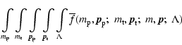
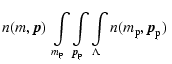
The disk is fully characterized by the distribution function
![]() ,
defined in such a way that
,
defined in such a way that
![]() is the number of particles with
is the number of particles with
![]() ,
,
![]() present in the disk at a certain instant of time t. The equation for the
distribution function n has the form (Krivov et al. 2005)
present in the disk at a certain instant of time t. The equation for the
distribution function n has the form (Krivov et al. 2005)
As discussed in Krivov et al. (2005),
![]() must not necessarily consist of all six Keplerian elements.
We can split all six into a vector of "important'' elements
must not necessarily consist of all six Keplerian elements.
We can split all six into a vector of "important'' elements ![]() and
a vector of "unimportant'' elements
and
a vector of "unimportant'' elements ![]() .
The letter
.
The letter ![]() in Eq. (4)-(6) can simply be replaced
with the letter
in Eq. (4)-(6) can simply be replaced
with the letter ![]() .
The equations will still be valid,
only the interpretation of quantities slightly changes.
The distribution n should now be understood as a
distribution averaged over the remaining elements
.
The equations will still be valid,
only the interpretation of quantities slightly changes.
The distribution n should now be understood as a
distribution averaged over the remaining elements ![]() .
Other quantities in integrands of (5) and (6),
too, are averages over qs.
In this case, we use
.
Other quantities in integrands of (5) and (6),
too, are averages over qs.
In this case, we use
![]() instead of f,
instead of f,
![]() instead of
instead of
![]() ,
and
,
and
![]() instead of
instead of ![]() .
They are formally defined
as integrals over qs. For instance, Dirac's
.
They are formally defined
as integrals over qs. For instance, Dirac's ![]() is replaced by
is replaced by
An important question is which
Keplerian elements of the six in total should be included in ![]() .
The more elements that are included in
.
The more elements that are included in ![]() ,
the more accurate the treatment, but
the required computational resources grow rapidly with the increasing
dimension of the phase space.
In this paper, we choose an idealized debris disk that
is rotationally-symmetric (uniformly distributed angular elements) and
geometrically thin (small orbital inclinations).
As a reasonable compromise, we therefore use
,
the more accurate the treatment, but
the required computational resources grow rapidly with the increasing
dimension of the phase space.
In this paper, we choose an idealized debris disk that
is rotationally-symmetric (uniformly distributed angular elements) and
geometrically thin (small orbital inclinations).
As a reasonable compromise, we therefore use ![]() with two elements:
semimajor axis a and eccentricity e.
Altogether, we have a three-dimensional (m, a, e) phase space.
with two elements:
semimajor axis a and eccentricity e.
Altogether, we have a three-dimensional (m, a, e) phase space.
In the original model (Krivov et al. 2005), averaging over
![]() s (inclination i, longitude of ascending node
s (inclination i, longitude of ascending node ![]() ,
longitude of pericenter
,
longitude of pericenter ![]() and an anomaly)
was "pre-done'' analytically before we started actual calculations with the model.
For instance, we found an approximate expression for (7).
and an anomaly)
was "pre-done'' analytically before we started actual calculations with the model.
For instance, we found an approximate expression for (7).
Here, we use a slightly different, and more accurate, method of averaging
over ![]() s and anomalies.
Consider two intersecting elliptic orbits (Fig. A.2).
In the 2D approximation such two ellipses always cross twice or graze once.
The relative orientation of the two orbits is given by the difference
of their longitudes of pericenters:
s and anomalies.
Consider two intersecting elliptic orbits (Fig. A.2).
In the 2D approximation such two ellipses always cross twice or graze once.
The relative orientation of the two orbits is given by the difference
of their longitudes of pericenters:
![]() .
For this reason, we simply add one more argument,
.
For this reason, we simply add one more argument, ![]() ,
to the functions
,
to the functions
![]() ,
,
![]() ,
and
,
and
![]() ,
and perform one additional (innermost)
integration over
,
and perform one additional (innermost)
integration over ![]() ,
in Eqs. (5) and (6).
Having
,
in Eqs. (5) and (6).
Having ![]() as an argument of functions is convenient
because
as an argument of functions is convenient
because ![]() immediately determines the true anomaly
immediately determines the true anomaly
The final equations have the form
![\begin{figure}
\par\includegraphics[width=14cm]{fi3.eps} \end{figure}](/articles/aa/full/2006/32/aa4907-06/img106.gif) |
Figure 3:
Fragments' orbits produced by collision of two particles
(
|
| Open with DEXTER | |
Initially, a cloud of fragments, produced by a disruptive collision, carries the
sum of the momenta of both colliders in one direction.
The fragments have zero
relative velocities, as we assume maximal collisional damping.
The resulting momentum is that of the center of mass and, in the 2D case, is
described by two conservation laws, one for the radial component and one for the
angular:
| (12) | |||
| (13) |
| p = a(1-e2), | (15) |
 |
(16) |
The masses of fragments produced by the collision are supposed to range
from arbitrarily small vapor particles to a certain upper limit
![]() ,
which is
determined by the properties of the parent bodies and their impact velocity
(e.g., Paolicchi et al. 1996):
,
which is
determined by the properties of the parent bodies and their impact velocity
(e.g., Paolicchi et al. 1996):
| (23) |
The fragment-generating function
![]() that enters
Eq. (10) describes the number of fragments with
that enters
Eq. (10) describes the number of fragments with
![]() that are
produced by a destructive collision of parent bodies with
that are
produced by a destructive collision of parent bodies with
![]() and
and
![]() .
It is a product of two distributions:
.
It is a product of two distributions:
| (24) |
| (25) |
![\begin{displaymath}\delta[a - a(m_{\rm p},{\vec p}_{\rm p};\:m_{\rm t},{\vec p}_{_{\rm t}};\:m;\:\Lambda)]
\end{displaymath}](/articles/aa/full/2006/32/aa4907-06/img148.gif) |
(26) |
![\begin{displaymath}\delta[e - e(m_{\rm p},{\vec p}_{\rm p};\:m_{\rm t},{\vec p}_{_{\rm t}};\:m;\:\Lambda)],
\end{displaymath}](/articles/aa/full/2006/32/aa4907-06/img149.gif) |
(27) |
 |
(28) |
The "geometric probability'' of collision
![]() (dimension: reciprocal of volume) and
the impact velocity
(dimension: reciprocal of volume) and
the impact velocity
![]() for two given elliptic orbits with a given angle
for two given elliptic orbits with a given angle ![]() between their
apsidal lines are
between their
apsidal lines are
To account for the third dimension, the impact velocity is calculated using an
average crossing angle:
| (31) |
For a derivation of these equations see the Appendix.
The collisional probabilities ![]() and velocities
and velocities
![]() are, as far as
possible, computed only once, and then used to calculate the gain and loss terms
for each time step, describing the destruction of parent bodies and the creation
of fragments.
Explicitly, for every bound orbit (
are, as far as
possible, computed only once, and then used to calculate the gain and loss terms
for each time step, describing the destruction of parent bodies and the creation
of fragments.
Explicitly, for every bound orbit (
![]() )
the distance r at which a
possible collision with another orbit (
)
the distance r at which a
possible collision with another orbit (
![]() )
would take place is
calculated at equidistant steps of the true anomaly
)
would take place is
calculated at equidistant steps of the true anomaly
![]() .
If the projectile p
reaches this distance during its revolution around the star, the following
quantities are calculated: the true anomalies
.
If the projectile p
reaches this distance during its revolution around the star, the following
quantities are calculated: the true anomalies
![]() and
and
![]() (Fig. A.2), together with
(Fig. A.2), together with
![]() ,
the instantaneous orbital velocities
,
the instantaneous orbital velocities ![]() and
and ![]() for the
case where
for the
case where
![]() ,
and the effective crossing angles
,
and the effective crossing angles
![]() .
These values, which are described in the Appendix, are stored.
Then at each time step for each crossing combination of orbits and each
combination of colliders' masses the discrete range of anomalies
.
These values, which are described in the Appendix, are stored.
Then at each time step for each crossing combination of orbits and each
combination of colliders' masses the discrete range of anomalies
![]() with
stored values is processed. The orbital velocities are properly scaled by
with
stored values is processed. The orbital velocities are properly scaled by
![]() and
and
![]() to determine the relative impact
velocity, and momentum
conservation is applied to obtain the orbits of all possible fragments up to the
limiting mass
to determine the relative impact
velocity, and momentum
conservation is applied to obtain the orbits of all possible fragments up to the
limiting mass
![]() which is calculated using
which is calculated using
![]() .
A linear
interpolation between the
.
A linear
interpolation between the
![]() -steps is used to distribute the fragments over
the (m,a,e)-grid. This selection of fragment orbits and the distribution of
mass together give the implementation of the fragment-generating function
-steps is used to distribute the fragments over
the (m,a,e)-grid. This selection of fragment orbits and the distribution of
mass together give the implementation of the fragment-generating function
![]() .
.
The abundance of grains on unbound orbits, ![]() -meteoroids, is
calculated as the product of their production rate and the average time it takes
for them to leave the disk, starting from the pericenter of their orbits.
-meteoroids, is
calculated as the product of their production rate and the average time it takes
for them to leave the disk, starting from the pericenter of their orbits.
The so-called Vega phenomenon for main-sequence stars
refers to a mid-infrared excess in the observed spectrum over
the purely stellar emission.
It was discovered in 1983 by the IRAS mission, at first for Vega itself
(Aumann et al. 1984), and was soon attributed to a
population of cold dust surrounding the star.
From the analysis of the spectral energy distribution in the spectral
range from 12
![]() (Aumann et al. 1984; Beichman et al. 1988) to 1.3 mm
(Chini et al. 1990),
conclusions about the properties of the assumed disk were made,
for instance the existence of an inner gap was inferred from the absence of
hot grains. The first spatially resolved submillimeter images of the Vega disk
were obtained with the SCUBA camera on the JCMT on Hawaii (Holland et al. 1998),
followed by other groups (Koerner et al. 2001; Wilner et al. 2002), who concentrated
on finding asymmetries. Recently, Su et al. (2005) observed the Vega system
at 24, 70, and 160
(Aumann et al. 1984; Beichman et al. 1988) to 1.3 mm
(Chini et al. 1990),
conclusions about the properties of the assumed disk were made,
for instance the existence of an inner gap was inferred from the absence of
hot grains. The first spatially resolved submillimeter images of the Vega disk
were obtained with the SCUBA camera on the JCMT on Hawaii (Holland et al. 1998),
followed by other groups (Koerner et al. 2001; Wilner et al. 2002), who concentrated
on finding asymmetries. Recently, Su et al. (2005) observed the Vega system
at 24, 70, and 160
![]() with the Spitzer space telescope and found radial
profiles of the Vega disk to be nearly rotationally symmetric and featureless.
The absence of asymmetries and substructure in the infrared makes the Vega disk
an ideal application of our approach.
with the Spitzer space telescope and found radial
profiles of the Vega disk to be nearly rotationally symmetric and featureless.
The absence of asymmetries and substructure in the infrared makes the Vega disk
an ideal application of our approach.
We set the initial size distribution to the well-known relation
![]() ,
starting at a minimum radius of
,
starting at a minimum radius of
![]()
![]() .
The total mass strongly depends on the upper mass cut-off (proportional to
.
The total mass strongly depends on the upper mass cut-off (proportional to
![]() ). To conform with previous mass estimates
(Holland et al. 1998; Su et al. 2005), the total observable mass was set to
be made up of grains up to a limiting radius of 1.5 mm. Grains larger than this
- the population of parent bodies - follow the same power law, but deliver
additional mass. The mass range used was 10-14 g to
). To conform with previous mass estimates
(Holland et al. 1998; Su et al. 2005), the total observable mass was set to
be made up of grains up to a limiting radius of 1.5 mm. Grains larger than this
- the population of parent bodies - follow the same power law, but deliver
additional mass. The mass range used was 10-14 g to
![]() g.
Thus, setting an observable
mass of
g.
Thus, setting an observable
mass of ![]() 0.5
0.5
![]() (lunar masses)
leads to a total initial mass of close to
300
(lunar masses)
leads to a total initial mass of close to
300
![]() or 3.5
or 3.5 ![]() (earth masses).
This range was covered by a grid of 70 bins with logarithmic steps with a step
factor of 2.6. The equivalent size grid has steps with factors of 1.37.
(earth masses).
This range was covered by a grid of 70 bins with logarithmic steps with a step
factor of 2.6. The equivalent size grid has steps with factors of 1.37.
To model the distribution of orbital elements,
from which then the spatial distribution of dust material was calculated,
we used a mesh of the semimajor axes from -400 to 400 AU with steps
of 20 AU, and eccentricity bins from -3 to 3 with width of 0.125, as depicted in
Fig. 8.
According to Su et al. (2005) and Dent et al. (2000), for the Vega disk we
adopted an initial distribution of semimajor axes between 80 AU to 120 AU,
chosen in such a way that for zero eccentricities the normal optical depth ![]() in this
distance range would be constant.
The distribution of semimajor axes outside a = 120 AU was taken to be a power law,
corresponding to the optical depth
in this
distance range would be constant.
The distribution of semimajor axes outside a = 120 AU was taken to be a power law,
corresponding to the optical depth
![]() .
Different values of the index
.
Different values of the index ![]() were tested, see below.
No material was placed initially inside a = 80 AU.
The initial distribution of eccentricities both in the "ring'' between 80 AU and 120 AU
and in the outer disk outside 120 AU was set uniform from zero to an upper limit
of
were tested, see below.
No material was placed initially inside a = 80 AU.
The initial distribution of eccentricities both in the "ring'' between 80 AU and 120 AU
and in the outer disk outside 120 AU was set uniform from zero to an upper limit
of
![]() or 3/8, depending on the run.
The vertical extension of the disk is defined by a
full-opening angle, which we arbitrarily set to
or 3/8, depending on the run.
The vertical extension of the disk is defined by a
full-opening angle, which we arbitrarily set to
![]() .
.
The optical and mechanical properties of dust in the disk are wildly unknown,
and we use here two types of grains: "rocky'' and "icy'' ones.
Assuming a mixture of 70% astronomical silicate of 3.5 g/cm3(Laor & Draine 1993), 30% amorphous carbon of 1.85 g/cm3(Zubko et al. 1996) and porosity close to zero, the effective grain bulk
density used here for "rocky'' grains is 3.0 g/cm3. The mean radiation
pressure efficiency
![]() ,
describing the momentum transfer from
radiation to grain, is set to unity.
The dependence of the critical energy for disruption on the grain size is given
by Eq. (22). The value of
,
describing the momentum transfer from
radiation to grain, is set to unity.
The dependence of the critical energy for disruption on the grain size is given
by Eq. (22). The value of
![]() at a size of 1 m was
set to 106 erg/g, and the slope
at a size of 1 m was
set to 106 erg/g, and the slope
![]() for this strength regime was set
to -0.24, although these values are not well defined by theoretical and
laboratory work.
To check how strongly the results depend on the adopted material,
one run was done for "icy'' grains of low bulk density (1 g/cm3)
and mechanical strength (
for this strength regime was set
to -0.24, although these values are not well defined by theoretical and
laboratory work.
To check how strongly the results depend on the adopted material,
one run was done for "icy'' grains of low bulk density (1 g/cm3)
and mechanical strength (
![]() erg/g at a size of 1 m).
In Eq. (21), we used c=1.24 for rock (Paolicchi et al. 1996)
and c=0.91 for ice (Arakawa 1999).
erg/g at a size of 1 m).
In Eq. (21), we used c=1.24 for rock (Paolicchi et al. 1996)
and c=0.91 for ice (Arakawa 1999).
The resulting dust distributions show strong fingerprints of the radiation
pressure. The most noticeable is the peak at the particle size where
![]() ,
so that the radiation pressure equals gravity (cf. Fig. 2). Below this size bound
orbits are impossible (Fig. 4), and the grains are blown away
on a timescale of the order of 102 to 103 years. Due to this lack of
possible impactors, grains slightly above this size limit are
overabundant, thereby reducing the number of grains of the next larger
population, and so on.
This dependence produces a well-known wavy pattern in the size or mass
distribution (e.g., Campo Bagatin et al. 1994; Durda & Dermott 1997; Thébault et al. 2003),
whose "wavelength'' depends on the ratio of the average impact energy available and
the impact energy
,
so that the radiation pressure equals gravity (cf. Fig. 2). Below this size bound
orbits are impossible (Fig. 4), and the grains are blown away
on a timescale of the order of 102 to 103 years. Due to this lack of
possible impactors, grains slightly above this size limit are
overabundant, thereby reducing the number of grains of the next larger
population, and so on.
This dependence produces a well-known wavy pattern in the size or mass
distribution (e.g., Campo Bagatin et al. 1994; Durda & Dermott 1997; Thébault et al. 2003),
whose "wavelength'' depends on the ratio of the average impact energy available and
the impact energy
![]() needed to disrupt a given target. The first is
controled by impact velocities, which depend on the disk's layout. The range of
inclinations and especially the range of eccentricities are important, because
they determine the orbits' crossing angles. The critical energy
needed to disrupt a given target. The first is
controled by impact velocities, which depend on the disk's layout. The range of
inclinations and especially the range of eccentricities are important, because
they determine the orbits' crossing angles. The critical energy
![]() ,
on
the other hand, is determined by material properties.
,
on
the other hand, is determined by material properties.
![\begin{figure}
\par\psfrag{YAxisLabel}[c][c]{$\frac{\mbox{cross section density}...
...ain radius [$\rm\mu m$ ]}
\includegraphics[width=8.8cm]{4907f4.eps} \end{figure}](/articles/aa/full/2006/32/aa4907-06/img186.gif) |
Figure 4:
Grain size distribution at 100 AU after 10 Myr for a rocky disk with
an initial outer profile
|
| Open with DEXTER | |
![\begin{figure}
\par\psfrag{YAxisLabel}[c][c]{$\frac{\mbox{cross section density}...
...ain radius [$\rm\mu m$ ]}
\includegraphics[width=8.8cm]{4907f5.eps} \end{figure}](/articles/aa/full/2006/32/aa4907-06/img187.gif) |
Figure 5: Grain size distribution at 100 AU and 10 Myr (4.5 Myr for "ice'') for different eccentricity ranges: 0.0 to 0.375 for "rock'' and "ice'', and only 0.0 to 0.125 for "circular'' orbits. The dashed lines are rescaled to coincide with the solid at large radii. The horizontal shift of the maximum for icy grains is largely due to a different bulk density. |
| Open with DEXTER | |
![\begin{figure}
\par\psfrag{YAxisLabel}[c][c]{$\frac{\mbox{cross section
density}...
...ain radius [$\rm\mu m$ ]}
\includegraphics[width=8.8cm]{4907f6.eps} \end{figure}](/articles/aa/full/2006/32/aa4907-06/img188.gif) |
Figure 6: Evolution of the size distribution of the disk of Fig. 4 at a distance of 100 AU. |
| Open with DEXTER | |
![\begin{figure}
\par\psfrag{YAxisLabel}[c][c]{$\frac{\mbox{cross section
density}...
...ain radius [$\rm\mu m$ ]}
\includegraphics[width=8.8cm]{4907f7.eps} \end{figure}](/articles/aa/full/2006/32/aa4907-06/img189.gif) |
Figure 7: Grain size distribution at distances from 50 AU to 350 AU in steps of 50 AU after 30 Myr. The initial disk is the same as in Fig. 4. The inner boundary of semimajor axes was placed at 80 AU. Therefore, only a small fraction of grains on sufficiently eccentric orbits contribute to the density at 50 AU. |
| Open with DEXTER | |
As is shown in Fig. 5 the disk's and the dust's set-up can have a noticeable influence on the size distribution. Low maximum eccentricities shorten the pattern's wavelength due to lower impact velocities leading to the critical impactor's size coming closer to the given target's. In contrast, the fluffy constitution of icy grains enlarges the gap between the target mass and the mass needed to disrupt it at a given impact velocity. Furthermore, it shifts the lower cut-off of the particle radius to higher values, according to the ratio of bulk densities, which is here 3:1. We note that a realistic disk cannot be built up of a perfectly homogeneous material, which implies a dispersion of densities, fragmentation energies etc. This could weaken or smear the waviness of the size distribution.
The time evolution of a particle size distribution of a modeled Vega disk is shown in Fig. 6. The larger the particles, the longer the collisional timescales, and the more time it takes for the size distribution to deviate significantly from the initial power law and to converge towards a quasi-steady state distribution whose absolute values are subject to change due to the amount of material delivered by collisions of larger bodies. Similarly, the comparison of different radial distances at the same time (Fig. 7) shows slower evolution at regions that are farther out with lower number densities and decreased impact velocities, where the latter also result in a reduced wavelength of the pattern.
Because we use the semimajor axis a and the eccentricity e as variables,
all quantities involving the radial distance r are computed by integrating
the distributions (cf. Krivov et al. 2005, Eq. (2.18)) over all the
orbits crossing or grazing this distance.
The actual distribution of the cross sectional area over the phase space of
a and e is plotted in Fig. 8 for rocky material with an
initial maximum eccentricity of 0.375 and a radial slope
![]() .
Near the
inner edge of the disk this surface area is dominated by eccentricities in the
range of the parent population's, whereas in the outer region the maximum
contribution comes from small grains on more eccentric orbits, because a higher
eccentricity at the same semimajor axis implies an origin closer to the star,
where the density of parent bodies is higher. Thus, the fragments created near
the disk's inner edge produce the main portion of optical depth out to a
considerable distance, setting an upper limit to the radial slope
.
Near the
inner edge of the disk this surface area is dominated by eccentricities in the
range of the parent population's, whereas in the outer region the maximum
contribution comes from small grains on more eccentric orbits, because a higher
eccentricity at the same semimajor axis implies an origin closer to the star,
where the density of parent bodies is higher. Thus, the fragments created near
the disk's inner edge produce the main portion of optical depth out to a
considerable distance, setting an upper limit to the radial slope ![]() .
Even
a ring-like or toroidal parent population with a sharp outer cut-off would lead
to a slope not steeper than this.
.
Even
a ring-like or toroidal parent population with a sharp outer cut-off would lead
to a slope not steeper than this.
![\begin{figure}
\par\psfrag{eccentricity}[bc][bc]{Eccentricity $e$ }
\psfrag{sem...
...ajor axis $a$\space [AU]}
\includegraphics[width=8.8cm]{4907f8.eps} \end{figure}](/articles/aa/full/2006/32/aa4907-06/img191.gif) |
Figure 8: The phase space distribution for the Vega disk of Fig. 4 at a quasi-steady state after 10 Myr. Each bin in the e-a-grid represents the surface area (in cm2 per phase space bin-volume) covered by the grains of all masses belonging to it. |
| Open with DEXTER | |
![\begin{figure}
\par\psfrag{YAxisLabel}[c][c]{normal optical depth}
\psfrag{XAxi...
...c]{distance to Vega [AU]}
\includegraphics[width=8.8cm]{4907f9.eps} \end{figure}](/articles/aa/full/2006/32/aa4907-06/img192.gif) |
Figure 9:
Radial profiles of the normal optical depth after 10 Myr:
one for an initially ring-like disk only (solid),
one for the ring followed by the semimajor axis distribution
|
| Open with DEXTER | |
The radial distribution of the optical depth at the end of the integration is shown in Fig. 9 for four different runs, corresponding to the source ring of constant surface density with and without adjacent outer part with different slopes and assuming different eccentricity distributions. As can be seen, the average slopes of all four profiles are comparable inside and outside the ring, which is located at 80-120 AU. The average outer slope is 1.5, but the ring-only configuration drops more sharply at the edge of the ring (1.7) and flattens more at larger distances (1.2), thereby deviating more strongly from a single power law. This flattening is caused partly by the fact that the outermost semimajor axis bin is overpopulated, because it represents orbits from 380 AU to infinity. The two power-law profiles make a smoother turn-over.
The convergence of one such radial profile towards a steady state
is illustrated in Fig. 10. This plot demonstrates the
transition from a steep profile
![]() with
with
![]() (corresponds to
(corresponds to
![]() )
to a
flattened one with
)
to a
flattened one with
![]() .
At the beginning of the simulation, the optical depth grows, reflecting overproduction
of the smallest
.
At the beginning of the simulation, the optical depth grows, reflecting overproduction
of the smallest ![]() -meteoroids, i.e. development of the primary maximum
in the wavy size distibution (Fig. 6).
Then the optical depth starts to decrease, due to ongoing collisional depletion
of large bodies and therefore decreased production of collisional fragments
at dust sizes.
The figure also shows how the radial location
of the peak optical depth is shifted outward due to higher rates of mass loss
in the inner regions.
-meteoroids, i.e. development of the primary maximum
in the wavy size distibution (Fig. 6).
Then the optical depth starts to decrease, due to ongoing collisional depletion
of large bodies and therefore decreased production of collisional fragments
at dust sizes.
The figure also shows how the radial location
of the peak optical depth is shifted outward due to higher rates of mass loss
in the inner regions.
![\begin{figure}
\par\psfrag{YAxisLabel}[c][c]{normal optical depth}
\psfrag{XAxi...
...]{distance to Vega [AU]}
\includegraphics[width=8.8cm]{4907f10.eps} \end{figure}](/articles/aa/full/2006/32/aa4907-06/img197.gif) |
Figure 10: Convergence of the radial profile of the normal optical depth for a rocky disk with an outer slope of -4. |
| Open with DEXTER | |
The resulting steady-state slopes of surface density that we find, between 1 and 2,
have to be compared to observations.
For large grains in thermal equilibrium the temperature is proportional to
r-1/2.
For wavelengths much larger than the peak flux wavelength for grains
of 50-100 K (60-30
![]() ), the emitted black-body energy is proportional to
the temperature itself.
In this case, the total surface brightness I of the thermal emission,
which is a product of the surface density or the optical depth and the
intensity in the observed spectral range, varies as
), the emitted black-body energy is proportional to
the temperature itself.
In this case, the total surface brightness I of the thermal emission,
which is a product of the surface density or the optical depth and the
intensity in the observed spectral range, varies as
![]() .
At wavelengths close to the maximum of the Planck function, the maximum intensity
goes as the fifth power of the temperature, giving
.
At wavelengths close to the maximum of the Planck function, the maximum intensity
goes as the fifth power of the temperature, giving
![]() .
Therefore, a radial profile of surface brightness with
indexes in a broad range between about -2 and -4 may be consistent with our
model, depending on the temperature distribution and the wavelength of the
observations.
Su et al. (2005) report that the observed surface brightness follows a power
law with index
.
Therefore, a radial profile of surface brightness with
indexes in a broad range between about -2 and -4 may be consistent with our
model, depending on the temperature distribution and the wavelength of the
observations.
Su et al. (2005) report that the observed surface brightness follows a power
law with index ![]() 4 for wavelengths of 24 and 70
4 for wavelengths of 24 and 70
![]() ,
and
,
and ![]() 3.5 for 160
3.5 for 160
![]() .
They suggest that small particles,
.
They suggest that small particles, ![]() 2
2
![]() ,
which sweep out throught the disk with an ideal
,
which sweep out throught the disk with an ideal
![]() and, according to their
calculations, with
and, according to their
calculations, with
![]() ,
are responsible for the observed flux.
However, the latter contradicts our model:
the contribution of grains of 2
,
are responsible for the observed flux.
However, the latter contradicts our model:
the contribution of grains of 2
![]() is by two orders of magnitude less than that of
grains of 10
is by two orders of magnitude less than that of
grains of 10
![]() (Fig. 6).
Collisions of
(Fig. 6).
Collisions of ![]() -meteoroids with
-meteoroids with ![]() -meteoroids, which are neglected
here, could slow the escape or produce
more small fragments, thereby prolonging the effective residence time, but
probably not efficiently enough.
-meteoroids, which are neglected
here, could slow the escape or produce
more small fragments, thereby prolonging the effective residence time, but
probably not efficiently enough.
So, we expect the main contribution to come from ![]() -meteoroids,
i.e. 10
-meteoroids,
i.e. 10
![]() and larger grains.
As mentioned above, this may be compatible with the observations.
For a more conclusive comparison to the observational data, realistic
calculations of grain temperatures and thermal fluxes need to be applied to our results,
which is beyond the scope of this paper.
There are many other physical mechanisms that could affect the radial profiles.
For instance, the disk may not be in a steady state.
A single catastrophic event in the past may have occurred, whose remnants produce the main
fraction of the currently visible fragmented material.
The primordial population of fragments from this event is expected to spread soon over a
circumstellar ring, which resembles our initial situation. If the time elapsed after the event
were too short to reach the steady state, a steeper profile would be expected
(Fig. 10). The upper limit (from Fig. 10) for this time is of the
order of 106 to 107 yr.
and larger grains.
As mentioned above, this may be compatible with the observations.
For a more conclusive comparison to the observational data, realistic
calculations of grain temperatures and thermal fluxes need to be applied to our results,
which is beyond the scope of this paper.
There are many other physical mechanisms that could affect the radial profiles.
For instance, the disk may not be in a steady state.
A single catastrophic event in the past may have occurred, whose remnants produce the main
fraction of the currently visible fragmented material.
The primordial population of fragments from this event is expected to spread soon over a
circumstellar ring, which resembles our initial situation. If the time elapsed after the event
were too short to reach the steady state, a steeper profile would be expected
(Fig. 10). The upper limit (from Fig. 10) for this time is of the
order of 106 to 107 yr.
The radial profile may be steepened by a mechanism that continuously removes grains in orbits with higher eccentricities, for instance a planet interior or exterior to the belt of parent bodies. As the radial distribution for a dynamically cold disk with reduced eccentricities shows (Fig. 9), the absence of eccentric parent bodies, which could be explained by an inner planet, does not influence the final result. A simple cut-off criterion forbidding planet crossing orbits only for parent bodies would have no impact on the results, either, but a continuous removal of small fragments on orbits of high eccentricity and short pericentric distances, which exist (Fig. 7, 50 AU; Fig. 8), could steepen the profile. The influence of an outer planet could be similar.
Table 1:
Masses of the modeled disks producing
![]() of dust.
of dust.
The total masses of the model disks
are listed in Table 1 for different runs.
The "rocky'' disks are made up of grains from 0.1
![]() to 300 m, the
"icy'' particles span a size range from 0.14
to 300 m, the
"icy'' particles span a size range from 0.14
![]() to 430 m,
so that the same mass range is covered.
The given masses and loss rates for ice are probably less realistic,
as the real dust is assumed to be a mixture of silicates and
carbonaceous material.
As the mass-per-size-decade distribution (Fig. 11) shows, the
derived total mass, which determines the absolute values of ordinates, is very
sensitive to where the upper cut-off is set, especially when considering the wave
pattern.
The relative mass loss,
to 430 m,
so that the same mass range is covered.
The given masses and loss rates for ice are probably less realistic,
as the real dust is assumed to be a mixture of silicates and
carbonaceous material.
As the mass-per-size-decade distribution (Fig. 11) shows, the
derived total mass, which determines the absolute values of ordinates, is very
sensitive to where the upper cut-off is set, especially when considering the wave
pattern.
The relative mass loss,
![]() ,
shows that all disks provide enough
material to sustain the current debris production over at least 80 Myr up
to 2.8 Gyr.
A higher mass-loss rate of the icy disk stems from the fact that ice is easier to destroy
than rock (smaller
,
shows that all disks provide enough
material to sustain the current debris production over at least 80 Myr up
to 2.8 Gyr.
A higher mass-loss rate of the icy disk stems from the fact that ice is easier to destroy
than rock (smaller
![]() ,
smaller mcr, and therefore shorter collisional lifetimes).
The existence of even larger parent bodies would further prolong the
disk's half-life and increase the total mass, according to
,
smaller mcr, and therefore shorter collisional lifetimes).
The existence of even larger parent bodies would further prolong the
disk's half-life and increase the total mass, according to
![]() ,
if the mass distribution's power law still holds for that
regime.
To analyse the evolution of total mass with time, we chose
a rocky disk with a ring-only distribution of parent bodies with a maximum
radius of 5 km. Figure 12 depicts the resulting moderate mass loss
over a period of 2 Gyr. From the mass loss rate of a system in a steady state,
,
if the mass distribution's power law still holds for that
regime.
To analyse the evolution of total mass with time, we chose
a rocky disk with a ring-only distribution of parent bodies with a maximum
radius of 5 km. Figure 12 depicts the resulting moderate mass loss
over a period of 2 Gyr. From the mass loss rate of a system in a steady state,
![]() ,
where cM is a constant, we can deduce the dependence of
mass on time:
,
where cM is a constant, we can deduce the dependence of
mass on time:
While Su et al. (2005) estimate the current mass loss due to blow-out of small
grains as
![]() g/s or 3200
g/s or 3200 ![]() /Gyr, we conclude that mass-loss rates
of 1 to 20
/Gyr, we conclude that mass-loss rates
of 1 to 20 ![]() /Gyr (Table 1) are consistent with an
observed amount of 0.5
/Gyr (Table 1) are consistent with an
observed amount of 0.5
![]() of submillimeter-sized dust.
A linear extrapolation by 350 Myr back in time would lead to initital disk masses
several orders of magnitude below the 330-3300 Jupiter masses
given by Su et al. (2005). Their estimation is based on the short lifetime
of unbound
of submillimeter-sized dust.
A linear extrapolation by 350 Myr back in time would lead to initital disk masses
several orders of magnitude below the 330-3300 Jupiter masses
given by Su et al. (2005). Their estimation is based on the short lifetime
of unbound ![]() -meteoroids, which they assume to be responsible for the
observable flux. The lifetime of small
-meteoroids, which they assume to be responsible for the
observable flux. The lifetime of small ![]() -meteoroids on bound orbits is
determined by the rate of destructive collisions and is much longer for
optically thin disks.
Given the observed amount of material and the longer lifetime, the necessary
production rate and the total mass decrease to more plausible values.
-meteoroids on bound orbits is
determined by the rate of destructive collisions and is much longer for
optically thin disks.
Given the observed amount of material and the longer lifetime, the necessary
production rate and the total mass decrease to more plausible values.
![\begin{figure}
\par\psfrag{YAxisLabel}[c][c]{$\frac{\mbox{mass
density}}{\mbox{u...
...in radius [$\rm\mu m$ ]}
\includegraphics[width=8.8cm]{4907f11.eps} \end{figure}](/articles/aa/full/2006/32/aa4907-06/img210.gif) |
Figure 11: Mass distribution at 100 AU after 10 Myr for the same disk as in Fig. 4. |
| Open with DEXTER | |
![\begin{figure}
\par\psfrag{YAxisLabel}[c][c]{total mass [$M_\oplus$ ]}
\psfrag{...
...Label}[c][c]{time [Myr]}
\includegraphics[width=8.8cm]{4907f12.eps} \end{figure}](/articles/aa/full/2006/32/aa4907-06/img211.gif) |
Figure 12: Decay of the total mass of a rocky, initially ring-only disk (thick line) and its fits through Eq. (32) with t0 = 200 (dotted), 600 (thin solid), and 2000 Myr (dashed). The largest bodies in this simulation measured 5 km in radius. |
| Open with DEXTER | |
The subject of this paper is a "typical circumstellar debris disk''. Instead of including a large array of forces and effects in a sophisticated numerical code to get as realistic model as possible, we have chosen here to concentrate on a few fundamental physical effects and to develop a kind of a reference model. Our main interest was to identify several essential, generic properties of such a debris disk, driven by these effects.
We thus treat the disk as an idealized ensemble of dust particles, exposed to stellar gravity and direct radiation pressure and experiencing fragmenting collisions. Two other effects, often thought to be of primary importance - gas drag and Poynting-Robertson drag - intentionally, are not included, for the following reasons. In debris disks - as opposed to protoplanetary disks and possibly transitional disks - gas drag does not play a significant role, simply because there is not enough gas (Thébault & Augereau 2005). The Poynting-Roberston effect is usually not important either, since collisional timescales are typically much shorter than the Poynting-Robertson decay time (Wyatt 2005; Krivov et al. 2000).
We use a method that can be referred to as a "kinetic theory in orbital elements''. Solving a balance equation for material gain and loss, we obtain a three-dimensional distribution of mass, semimajor axes, and eccentricities, averaged over the other elements. This distribution can easily be transformed to "usual'' distributions, such as size distribution or radial profiles.
We have investigated what kind of size/mass and spatial distributions of the disk material can be expected from theory, and how these distributions might depend on the distributions of the parent bodies, parameters of the central star, and grain properties. With a number of tests, we have checked that the properties we found are generic. The model designed here may serve as a skeleton for the development of more complete models with a number of additional effects included: physical sources, drag mechanisms, more accurate impact physics with cratering collisions and restitution, etc.
An application is made to the disk around Vega. This disk is seen edge-on and appears nearly uniform, representing an ideal application of our model.
Our main findings are as follows:
Radiation pressure affects the distribution towards larger sizes as well. Overabundance or underabundance of smaller projectiles are repeatedly reflected at larger sizes, and thus, a kind of resonance comes into play, generating a wavy pattern in the size distribution. This might influence modeling of disk's spectral properties and disk mass estimates. The pattern is well understood (Campo Bagatin et al. 1994) as the result of the lower size cut-off produced by the blowout due to radiation pressure and was obtained by other models (Thébault et al. 2003), too. The reported peak at a grain size twice as large as the smallest bound grains is found as well as the lack of grains 20 to 100 times as large. However, the quantitative results differ, because the pattern's wavelength and amplitude strongly depend on the grains' mechanical properties and average impact velocities.
Acknowledgements
We wish to thank the anonymous referee for a thorough and helpful review. Miodrag Sremcevic is supported by the Cassini UVIS project.
Consider first a single particle flying a certain distance through an
ensemble of targets distributed at a given number density
![]() with an
interaction cross-section
with an
interaction cross-section ![]() .
The differential hit probability with
respect to x,
the distance flown, is given by
.
The differential hit probability with
respect to x,
the distance flown, is given by
![]() .
If, instead of a
single projectile, we consider a second ensemble of a given density
.
If, instead of a
single projectile, we consider a second ensemble of a given density
![]() ,
interacting with the target ensemble, we get the symmetric expression
,
interacting with the target ensemble, we get the symmetric expression
| |
Figure A.1:
Collision of two groups of particles in a small volume of interaction
|
The linear number density ![]() of projectiles and targets along their
orbits is determined by their phase space density n together with
the elementary phase space volume
of projectiles and targets along their
orbits is determined by their phase space density n together with
the elementary phase space volume
![]() and the Kepler
equation, which gives the individual orbital velocity v and the orbital period
P:
and the Kepler
equation, which gives the individual orbital velocity v and the orbital period
P:
| (A.3) |
 |
(A.4) |
![\begin{figure}
\includegraphics[width=8.8cm]{fiA2.eps}\end{figure}](/articles/aa/full/2006/32/aa4907-06/img254.gif) |
Figure A.2:
Two elliptic orbits crossing in 2D: (a) two cases for fixed difference
|
After separating the number densities, the impact velocity, the cross
section ![]() ,
and the differentials, the remaining term describes the
geometric probability of a collision of two such orbits, but averaged over all
variables not involved in the above calculations: the inclinations and the
absolute orientation of (one of) the orbits. This probability is of unit one
per volume and is very similar to the
,
and the differentials, the remaining term describes the
geometric probability of a collision of two such orbits, but averaged over all
variables not involved in the above calculations: the inclinations and the
absolute orientation of (one of) the orbits. This probability is of unit one
per volume and is very similar to the ![]() -integral in
Krivov et al. (2005), but without averaging over the relative positions of
both orbits - there is still a dependence on the distance to the star r at
which the collision occurs:
-integral in
Krivov et al. (2005), but without averaging over the relative positions of
both orbits - there is still a dependence on the distance to the star r at
which the collision occurs:
| (A.15) |
![\begin{figure}
\psfrag{YAxisLabelDel}[bc][bc]{$\Delta(a_{\rm p},e_{\rm p},a_{\rm...
...th=8.8cm]{4907fA3a.eps} \includegraphics[width=8.8cm]{4907fA3b.eps} \end{figure}](/articles/aa/full/2006/32/aa4907-06/img272.gif) |
Figure A.3:
The |
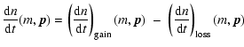
At this point we are able to evaluate the gain and loss terms (10) and
(11).
For example, the gain term can be written as
![$\displaystyle \left(
\frac{\ensuremath{{\rm d}} n}{\ensuremath{{\rm d}} t}
\rig...
...-} }v\ensuremath{_{\rm imp}} {\ensuremath{^-} }\Delta{\ensuremath{^-} }
\right]$](/articles/aa/full/2006/32/aa4907-06/img273.gif) |
|||
| (A.16) |
One gets the same result as in Eq. (A.18) by starting from Eq.
(7), reformulating the Dirac functions to depend on one
collider's longitude of the pericenter,
![]() ,
as well as
,
as well as
![]() and
and
![]() .
The Jacobian, transforming in 2D from the Cartesian case
.
The Jacobian, transforming in 2D from the Cartesian case
![]() to
to
![]() and
and
![]() ,
is given
by
,
is given
by
| J-1 | = |  |
|
| = |  |
(A.19) |
| |
= |  |
|
| = |  |
||
| = | (A.20) |
 |
(A.21) |


![$\displaystyle 2 - \frac{m_{\rm p}^2}{m\ensuremath{\ensuremath{_{\rm sum}}} ^2}\...
...} ^2}\cdot \frac{1-\beta_{\rm t}}{1-\beta}
\left[2 - \frac{r}{a_{\rm t}}\right]$](/articles/aa/full/2006/32/aa4907-06/img116.gif)
![$\displaystyle \pm \sqrt{\left(2 - \frac{r}{a_{\rm p}} - \frac{p_{\rm p}}{r}\right)
\left(2 - \frac{r}{a_{\rm t}} - \frac{p_{\rm t}}{r}\right)}\Bigg],$](/articles/aa/full/2006/32/aa4907-06/img118.gif)
![$\displaystyle \left.\left. + 2\frac{m_{\rm p}m_{\rm t}}{m\ensuremath{\ensuremat...
...\beta_{\rm t})}}
{1-\beta} \sqrt{p_{\rm p}p_{\rm t}}\right)\right]^\frac{1}{2}.$](/articles/aa/full/2006/32/aa4907-06/img120.gif)
![$\displaystyle m\ensuremath{_{\rm x}} =
\frac{m_{\rm t}}{2}\left[2\frac{m_{\rm t...
...math{_{\rm D}} ^*(m_{\rm t})}{\ensuremath{\overline{v_{\rm imp}}} ^2}\right]^c,$](/articles/aa/full/2006/32/aa4907-06/img128.gif)
![$\displaystyle \sqrt{GM(1-\beta\ensuremath{_{\rm p,t}} )\left[\frac{2}{r} -
\frac{1}{a\ensuremath{_{\rm p,t}} }\right]},$](/articles/aa/full/2006/32/aa4907-06/img235.gif)
![$\displaystyle \frac{1 + \left(\frac{1}{r}\frac{\partial r}{\partial\vartheta_{\...
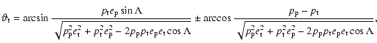
...left(\frac{1}{r}\frac{\partial r}{\partial\vartheta_{\rm t}}\right)^2\right]}},$](/articles/aa/full/2006/32/aa4907-06/img239.gif)
![$\displaystyle \frac{\left\vert\frac{1}{r}\frac{\partial r}{\partial\vartheta_{\...
...(\frac{1}{r}\frac{\partial r}{\partial\vartheta_{\rm t}}\right)^2\right]}}\cdot$](/articles/aa/full/2006/32/aa4907-06/img241.gif)
![$\displaystyle {\Delta ({\vec p}_{\rm p},{\vec p}_{\rm t};\; \vartheta_{\rm t})}...
...) \over a_{\rm p}} - {p_{\rm p}\over
r(\vartheta_{\rm t})}\right)}
\right]^{-1}$](/articles/aa/full/2006/32/aa4907-06/img277.gif)