A&A 455, 385-393 (2006)
DOI: 10.1051/0004-6361:20064992
F. Patat1 - O. S. Ugolnikov2 - O. V. Postylyakov3
1 - European Southern Observatory (ESO), K. Schwarzschildstr. 2,
85748, Garching b. München, Germany
2 -
Space Research Institute, Russian Academy of Sciences,
Profsoyuznaya ul., 84/32, Moscow, 117997 Russia
3 -
A.M.Obukhov's Institute of Atmospheric Physics, Russian
Academy of Sciences, Pyzhevsky per., 3, Moscow, 119017 Russia
Received 9 February 2006 / Accepted 10 April 2006
Abstract
Context. Twilight studies have proved to be important tools for analyzing the atmospheric structure with interesting consequences on the characterization of astronomical sites. Active discussions of this topic have started again recently in connection with the evaluation of Dome C, Antarctica, as a potential astronomical site and several site-testing experiments, including twilight brightness measurements, are being prepared.
Aims. The present work provides the first absolute photometric measurements of twilight sky brightness for ESO-Paranal (Chile). They are meant both as a contribution to the site monitoring and as reference values in the analysis of other sites, including Dome C.
Methods. The
![]() twilight sky brightness was estimated on more than 2000 FORS1 archival images, which include both flats and standard star observations taken in twilight and covering a Sun zenith distance range 94
twilight sky brightness was estimated on more than 2000 FORS1 archival images, which include both flats and standard star observations taken in twilight and covering a Sun zenith distance range 94![]() -112
-112![]() .
.
Results. The comparison with a low-altitude site shows that Paranal V twilight sky brightness is about 30% lower, implying that some fraction of multiple scattering has to take place at an altitude of a few km above sea level.
Key words: atmospheric effects - site testing - techniques: photometric
The quality of an astronomical site is determined by several parameters, which may vary according to the wavelength range of interest. For the optical and near-IR domain, these include typical seeing, sky transparency, number of clear nights, humidity, night sky brightness, amount of precipitable water vapor, dust, and aerosols. While the seeing, extinction, sky brightness, and other quantities are commonly measured at most observatories, the twilight brightness is not. This is mainly because the relevant information on the typical atmospheric conditions can be derived from other measurements obtained during the night. Nevertheless, twilight observations provide an independent tool for probing the overhead atmosphere under much higher flux conditions, thus allowing more accurate results. The interested reader can find an extensive review of this topic in the classical textbook by Rozenberg (1966).
Very recently, the twilight has received particular attention due to the growing interest of the international astronomical community for what seems to be the new frontier of ground-based astronomy, i.e. Dome C - Antarctica. This site is exceptional in many respects. Besides the extremely good seeing conditions reported by Lawrence et al. (2004), several studies have shown very low amounts of precipitable water vapor that, coupled with a low sky emission, could imply that this is the best site for IR and sub-millimetric ground-based astronomy. A review of the characteristics of Dome C has been recently presented by Kenyon & Storey (2005).
One of the main concerns is related to the high latitude of this site. This, in fact, causes a significant reduction in the amount of dark time with respect to equatorial observatories, thus posing some doubts about the effective exploitation of the exceptional seeing in the optical. The possibility of opening spectral windows otherwise inaccessible from the ground is in itself a valid and sufficient scientific driver for Dome C. Nevertheless, arguments in favor of Dome C as a site for optical astronomy have been put forward. Among these, a smaller average contribution by the scattered moonlight to the global background and a cleaner atmosphere have been advocated as features that may possibly compensate for the reduced dark time (Kenyon & Storey 2005). In particular, since the last phases of twilight (also known as deep twilight) are dominated by multiple scattering (Rozenberg 1966), the amount of scattered sunlight is strongly dependent on the amount of aerosol in the lower atmospheric layers (see for example Ougolnikov et al. 2004). In a supposedly low aerosol content site like Dome C, this effect is expected to be very low, and it would, in turn, allow one to start the observations earlier than at normal sites. Even though the argument has a good physical ground, direct on-site measurements are still lacking. In this respect, it is worth mentioning that a couple of dedicated experiments for sky brightness measurements are currently being setup (A. Moore, J. Storey 2006, private communications).
In spite of the large number of investigations done in the past in
this field, absolute twilight brightness measurements are rather rare,
especially for large observatories placed in top-rated sites. To our
knowledge, the only published work on twilight observations in the
Johnson-Cousins standard system is the one by Tyson & Gal
(1993) who, given their purposes, report only uncalibrated
data for CTIO. In light of these facts, both with the purpose of also
characterizing Paranal from this new point of view and of providing
the community with absolute reference values obtained over a large
time baseline, we present here
![]() twilight sky brightness
measurements for the first time.
twilight sky brightness
measurements for the first time.
The paper is organized as follows. In Sect. 2 we
introduce the basic concepts through a simplified model (which is
discussed in more detail in Appendix A), while in Sect. 3
we describe the observations, data reduction, and calibration. The
![]() twilight sky brightness measured at ESO-Paranal is presented
and discussed in Sect. 4, while Sect. 5
summarizes the results obtained in this work.
twilight sky brightness measured at ESO-Paranal is presented
and discussed in Sect. 4, while Sect. 5
summarizes the results obtained in this work.
The calculation of scattered flux during twilight is a rather complicated problem that requires a detailed treatment of multiple scattering (see for example Blättner et al. 1974; Wu & Lu 1988) and an accurate description of the atmospheric composition and the physical phenomena taking place in the various layers (Divari & Plotnikova 1966; Rozenberg 1966). Notwithstanding the large amount of work done in the '60s and in the '70s, the problem is still a matter of investigations (see for example Anderson & Lloyd 1990; Ougolnikov 1999; Ougolnikov & Maslov 2002; Ekstrom 2002; Ougolnikov et al. 2004; Postylyakov 2004; Mateshvili et al. 2005). While it is well beyond the purposes of the present work to explore the problem from a theoretical point of view, we deemed it interesting to introduce a simple single-scattering model, which is useful both for understanding the basic principles of twilight and to providing a quick comparison to the observed data. The assumptions and the model itself are discussed in Appendix A, to which we refer the interested reader for the details, while here we concentrate on the model predictions only.
The calculated zenith (![]() )
)
![]() sky brightness as a
function of Sun zenith distance
sky brightness as a
function of Sun zenith distance ![]() ,
computed using the average
broad band extinction coefficients for Paranal (Patat
2003a), are plotted in Fig. 1.
As one can immediately see, the single scattering component drops
below the night sky brightness between
,
computed using the average
broad band extinction coefficients for Paranal (Patat
2003a), are plotted in Fig. 1.
As one can immediately see, the single scattering component drops
below the night sky brightness between ![]()
![]() and
and
![]() ,
indicating that from this point on multiple
scattering is the only contributor to the observed flux, as shown by
Ugolnikov & Maslov (2002) on the basis of polarization
measurements.
,
indicating that from this point on multiple
scattering is the only contributor to the observed flux, as shown by
Ugolnikov & Maslov (2002) on the basis of polarization
measurements.
![\begin{figure}
\par\includegraphics[width=7.2cm,clip]{4992fg01.eps}
\end{figure}](/articles/aa/full/2006/31/aa4992-06/img17.gif) |
Figure 1: Model twilight sky brightness at zenith. The thick curves include the night sky contribution, while the thin lines indicate only the scattered component. The vertical dashed-dotted line marks the Sun zenith distance when the lower boundary layer height is 120 km. The upper scale indicates the lower Earth's boundary layer height in km. |
| Open with DEXTER | |
Another aspect to be considered is that the transition to the flatter
part of the atmospheric density profile (see Fig. A.2)
definitely occurs during the multiple scattering-dominated
phase. Since multiple scattering takes place with higher probability
where the density is higher, i.e. in the lower atmospheric layers, the
explanation given by Tyson & Gal (1993) for the observed rate
of decline in brightness during twilight does not seem to be correct.
In fact, these authors interpret the observed values as the pure
consequence of the lower shadow boundary height change, neglecting
extinction and multiple scattering. They conclude that, since their
observations have been taken when
![]() km (where hz is the height of the lower Earth's shadow boundary along the
zenith direction; see also Appendix A), the sky brightness rate is
directly related to the slope of the density law in that region of the
atmosphere. Nevertheless, calculation of the Sun's ephemeris for the
site and epoch of Tyson & Gal's observations shows that, in the most
extreme case (see their Table 1, R filter), it was 1
km (where hz is the height of the lower Earth's shadow boundary along the
zenith direction; see also Appendix A), the sky brightness rate is
directly related to the slope of the density law in that region of the
atmosphere. Nevertheless, calculation of the Sun's ephemeris for the
site and epoch of Tyson & Gal's observations shows that, in the most
extreme case (see their Table 1, R filter), it was 1![]() .
.
![]()
![]() . 4 (where
. 4 (where
![]() ). As the reader can
figure out from Table A.1, this implies that hz<80 km
in all cases, i.e. well within the steep part of the density
profile. Therefore, that the observed rate and the rate expected from
pure single scattering in the higher atmospheric layers are consistent
is just a coincidence.
). As the reader can
figure out from Table A.1, this implies that hz<80 km
in all cases, i.e. well within the steep part of the density
profile. Therefore, that the observed rate and the rate expected from
pure single scattering in the higher atmospheric layers are consistent
is just a coincidence.
In order to measure the twilight sky brightness on Paranal, we used
archival calibration data obtained with the FOcal
Reducer/low-dispersion Spectrograph (hereafter FORS1), mounted at the
Cassegrain focus of the ESO-Antu/Melipal 8.2 m telescopes (Szeifert
2002). The instrument is equipped with a
![]() pixel (px)
TK2048EB4-1 backside-thinned CCD and has two remotely exchangeable
collimators, which give a projected scale of 0
pixel (px)
TK2048EB4-1 backside-thinned CCD and has two remotely exchangeable
collimators, which give a projected scale of 0
![]() 2 and 0
2 and 0
![]() 1 per pixel
(24
1 per pixel
(24 ![]() m
m ![]() 24
24 ![]() m). According to this collimator, the sky
area covered by the detector is 6
m). According to this collimator, the sky
area covered by the detector is 6![]() . 8
. 8 ![]() 6
6![]() . 8 and
3
. 8 and
3![]() . 4
. 4 ![]() 3
3![]() . 4. For this study we selected only the data obtained
with the lower resolution collimator and the 4-port high-gain read-out
mode, since this combination is used the most for imaging with
FORS1. The read-out noise is 5.5 electrons (e-) with this setup.
. 4. For this study we selected only the data obtained
with the lower resolution collimator and the 4-port high-gain read-out
mode, since this combination is used the most for imaging with
FORS1. The read-out noise is 5.5 electrons (e-) with this setup.
For our purposes, we selected two sets of data. The first is composed
of broad-band
![]() twilight sky flats (hereafter TSF), which are
regularly obtained as part of the calibration plan. In the current
implementation, the observing software estimates with a simple
algorithm the integration time for the first exposure in a series of 4 frames after taking a test exposure. Subsequent exposure times are
adjusted on the basis of the previous exposure level and this allows
one to obtain high signal-to-noise images with a rather constant
count level, which is typically around 20 000 ADUs. This is achieved
with exposure times that range from 0.25 s up to 5 min. Given
these values, the sensitivity of FORS1 in the various passbands and
the typical twilight sky brightness behavior (see for example
Fig. 1), these observations are expected to
approximately cover the Sun zenith distance range
94
twilight sky flats (hereafter TSF), which are
regularly obtained as part of the calibration plan. In the current
implementation, the observing software estimates with a simple
algorithm the integration time for the first exposure in a series of 4 frames after taking a test exposure. Subsequent exposure times are
adjusted on the basis of the previous exposure level and this allows
one to obtain high signal-to-noise images with a rather constant
count level, which is typically around 20 000 ADUs. This is achieved
with exposure times that range from 0.25 s up to 5 min. Given
these values, the sensitivity of FORS1 in the various passbands and
the typical twilight sky brightness behavior (see for example
Fig. 1), these observations are expected to
approximately cover the Sun zenith distance range
94
![]() ,
i.e. still within the nautical twilight. Since the
most important part of this analysis concerns the deep twilight, it
is clear that an additional set of data is required to complement the
sky flats.
,
i.e. still within the nautical twilight. Since the
most important part of this analysis concerns the deep twilight, it
is clear that an additional set of data is required to complement the
sky flats.
The calibration plan of FORS1 includes the observation of standard
star fields (Landolt 1992) in
![]() passbands, which are
regularly taken during twilight, typically just after the sky flat
sequence is completed. For calibration purposes, a fraction of these
exposures are obtained using relatively long integration times
(typically 40 s for U and 20 s for
passbands, which are
regularly taken during twilight, typically just after the sky flat
sequence is completed. For calibration purposes, a fraction of these
exposures are obtained using relatively long integration times
(typically 40 s for U and 20 s for
![]() )
which, at an 8 m-class telescope, are sufficient to bring the sky background to
exposure levels that are suitable for our purposes. In fact, the bulk
of these observations covers the range 100
)
which, at an 8 m-class telescope, are sufficient to bring the sky background to
exposure levels that are suitable for our purposes. In fact, the bulk
of these observations covers the range 100
![]() ,
i.e. well into astronomical twilight.
For the sake of clarity we indicate them as long-exposure standards
(LES).
,
i.e. well into astronomical twilight.
For the sake of clarity we indicate them as long-exposure standards
(LES).
In order to collect a statistically significant sample, we
retrieved from the ESO Archive all suitable TSF obtained in
![]() passbands from 1 Jan. 2005 to 30 Sep. 2005, for a total of 1083 frames
(U: 148, B: 208, V: 226, R: 261, I: 240). Since a much higher
night-to-night spread is expected in the deep twilight phase due to
the natural fluctuations of the night sky emission and also because
LES are less frequently obtained than TSF, a longer time interval
must be considered. To this aim, we have put together the LES sample
collecting all suitable images obtained from 1 Jan. 1999 (i.e. shortly
after the beginning of FORS1 operations) to 30 Sep. 2005, thus covering
almost 6 years, for a total of 3388 frames (U: 923, B: 611, V: 609, R:
635, I: 610). All images were processed within the xccdred
package of IRAF
passbands from 1 Jan. 2005 to 30 Sep. 2005, for a total of 1083 frames
(U: 148, B: 208, V: 226, R: 261, I: 240). Since a much higher
night-to-night spread is expected in the deep twilight phase due to
the natural fluctuations of the night sky emission and also because
LES are less frequently obtained than TSF, a longer time interval
must be considered. To this aim, we have put together the LES sample
collecting all suitable images obtained from 1 Jan. 1999 (i.e. shortly
after the beginning of FORS1 operations) to 30 Sep. 2005, thus covering
almost 6 years, for a total of 3388 frames (U: 923, B: 611, V: 609, R:
635, I: 610). All images were processed within the xccdred
package of IRAF![]() . Due to the large amount of data and the
purpose of this work, the bias subtraction was performed using only a
pre-scan correction, while flat-fielding was achieved using a
stack of all TSF in each given passband as a master flat, which was
then adopted to correct each TSF and LES frame.
. Due to the large amount of data and the
purpose of this work, the bias subtraction was performed using only a
pre-scan correction, while flat-fielding was achieved using a
stack of all TSF in each given passband as a master flat, which was
then adopted to correct each TSF and LES frame.
Due to the nature of the data, there is no need to take care of the
possible presence of crowded stellar fields or bright extended
objects, as is the case for night sky brightness estimates (see
Patat 2003b). For this reason, the background in each image
was measured using a simple and robust mode estimator. To avoid
possible vignetting and flat-fielding problems, only the central
![]() pixels were considered. On these spatial scales and
due to improper flat-fielding, FORS1 is known to show variations on
the order of a few percent, while the gradients in the twilight sky
are much smaller (see Chromey & Hasselbacher
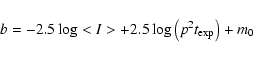
1996) and can be safely neglected. Therefore, the mode <I> of
pixel intensity distribution is assumed as the best estimate of the
sky background. For each filter, this is converted into a surface
brightness in the Johnson-Cousins system via the following relation
pixels were considered. On these spatial scales and
due to improper flat-fielding, FORS1 is known to show variations on
the order of a few percent, while the gradients in the twilight sky
are much smaller (see Chromey & Hasselbacher
1996) and can be safely neglected. Therefore, the mode <I> of
pixel intensity distribution is assumed as the best estimate of the
sky background. For each filter, this is converted into a surface
brightness in the Johnson-Cousins system via the following relation
![\begin{figure}
\par\includegraphics[width=7.3cm,clip]{4992fg02.eps}
\end{figure}](/articles/aa/full/2006/31/aa4992-06/img32.gif) |
Figure 2:
Distribution of twilight observations in Alt-Az
coordinates for TSF (filled symbols) and LSE (empty symbols). The
astronomical azimuth has been replaced with the difference in azimuth
between the telescope pointing and the Sun,
|
| Open with DEXTER | |
Since the data were not obtained specifically for twilight brightness
measurements, they are inhomogeneously distributed on the sky. In
fact, in an Alt-Az plot where the ordinary azimuth is replaced by the
difference in azimuth between the sky patch and the Sun (
![]() ), the data points tend to cluster in two
regions, which correspond to evening and morning observations
(Fig. 2). Besides target azimuth and altitude we
computed a series of other quantities for each data point, which are
relevant for the subsequent analysis. These include Sun azimuth and
altitude, Sun-target angular separation, Moon phase, Moon altitude, and
Moon-target angular separation. To avoid contamination from scattered
moonlight in the LSE, we selected only those data points for
which the Moon was below the horizon.
), the data points tend to cluster in two
regions, which correspond to evening and morning observations
(Fig. 2). Besides target azimuth and altitude we
computed a series of other quantities for each data point, which are
relevant for the subsequent analysis. These include Sun azimuth and
altitude, Sun-target angular separation, Moon phase, Moon altitude, and
Moon-target angular separation. To avoid contamination from scattered
moonlight in the LSE, we selected only those data points for
which the Moon was below the horizon.
Since the twilight sky brightness for a given Sun zenith distance
changes with the position on the sky, it is necessary to make a
selection on the Alt-Az coordinates to study its behavior as a
function of ![]() .
Given the nature of the available data, which
appear to be rather concentrated (Fig. 2), it seems
reasonable to restrict the analysis only to zenith region. In order to
have a sufficient amount of measurements, we used all data points
with zenith distance
.
Given the nature of the available data, which
appear to be rather concentrated (Fig. 2), it seems
reasonable to restrict the analysis only to zenith region. In order to
have a sufficient amount of measurements, we used all data points
with zenith distance
![]() ,
which is of course
expected to cause some additional spread in the observed relation.
The results are presented in Figs. 3-7 for
the
,
which is of course
expected to cause some additional spread in the observed relation.
The results are presented in Figs. 3-7 for
the
![]() passbands.
passbands.
![\begin{figure}
\par\includegraphics[width=6.8cm,clip]{4992fg03.eps}
\end{figure}](/articles/aa/full/2006/31/aa4992-06/img34.gif) |
Figure 3:
Zenith twilight sky surface brightness in the
U passband from TSF (empty symbols) and LSE (filled symbols) with
|
| Open with DEXTER | |
![\begin{figure}
\par\includegraphics[width=6.8cm,clip]{4992fg04.eps}
\end{figure}](/articles/aa/full/2006/31/aa4992-06/img35.gif) |
Figure 4: Same as Fig. 3 for the B passband. |
| Open with DEXTER | |
![\begin{figure}
\par\includegraphics[width=6.8cm,clip]{4992fg05.eps}
\end{figure}](/articles/aa/full/2006/31/aa4992-06/img36.gif) |
Figure 5: Same as Fig. 4 for the V passband. |
| Open with DEXTER | |
![\begin{figure}
\par\includegraphics[width=6.8cm,clip]{4992fg06.eps}
\end{figure}](/articles/aa/full/2006/31/aa4992-06/img37.gif) |
Figure 6: Same as Fig. 3 for the R pass band. |
| Open with DEXTER | |
![\begin{figure}
\par\includegraphics[width=6.8cm,clip]{4992fg07.eps}
\end{figure}](/articles/aa/full/2006/31/aa4992-06/img38.gif) |
Figure 7: Same as Fig. 3 for the I passband. |
| Open with DEXTER | |
As expected, the single scatter model drops much faster than the
actual observations. While for ![]() the model deviates from the data
around
the model deviates from the data
around
![]() ,
for B and especially for U the model
already underestimates the surface brightness at
,
for B and especially for U the model
already underestimates the surface brightness at
![]() ,
indicating that multiple scattering is more
efficient at shorter wavelengths. This agrees with the findings of
Ougolnikov & Maslov (2002), who show that the
contribution of single scattering in the phases immediately following
sunset is about 40%, 60%, 70%, and 80% in U, B, V, and R,
respectively. These fractions remain roughly constant until
,
indicating that multiple scattering is more
efficient at shorter wavelengths. This agrees with the findings of
Ougolnikov & Maslov (2002), who show that the
contribution of single scattering in the phases immediately following
sunset is about 40%, 60%, 70%, and 80% in U, B, V, and R,
respectively. These fractions remain roughly constant until
![]() ,
after which the role of single scattering
becomes weaker and weaker and multiple scattering rapidly takes
over. In all passbands, the night sky brightness level is reached at
around
,
after which the role of single scattering
becomes weaker and weaker and multiple scattering rapidly takes
over. In all passbands, the night sky brightness level is reached at
around
![]() .
.
In order to give a more quantitative description of the observations,
we fitted the surface-brightness data in the range 95
![]() using second order polynomials of the form
using second order polynomials of the form
![]() ,
with
,
with ![]() expressed in
degrees and the surface brightness in mag arcsec-2. The results
are presented in Table 1, where we also report the
RMS deviation from the fitted function
expressed in
degrees and the surface brightness in mag arcsec-2. The results
are presented in Table 1, where we also report the
RMS deviation from the fitted function ![]() and the slope
and the slope ![]() deduced from a linear fit to the data in the range 95
deduced from a linear fit to the data in the range 95
![]() ,
i.e. during the interval typically used to obtain
TSF exposures, when the contribution by the night sky is still
moderate. A first aspect to be noticed is the spread shown by the
data points around the mean laws, which is due to the night-to-night
variations in the atmospheric conditions. The dispersion becomes
particularly large in the I passband, where the fluctuations appear
to be quite pronounced. We notice that the decay rate during nautical
twilight tends to decrease for increasing values of wavelength.
,
i.e. during the interval typically used to obtain
TSF exposures, when the contribution by the night sky is still
moderate. A first aspect to be noticed is the spread shown by the
data points around the mean laws, which is due to the night-to-night
variations in the atmospheric conditions. The dispersion becomes
particularly large in the I passband, where the fluctuations appear
to be quite pronounced. We notice that the decay rate during nautical
twilight tends to decrease for increasing values of wavelength.
To convert the values of ![]() reported in
Table 1 into surface brightness variation per unit time,
one has to multiply them by
reported in
Table 1 into surface brightness variation per unit time,
one has to multiply them by
![]() ,
which is given by:
,
which is given by:
Table 1:
Twilight sky brightness fitted parameters in the
range 95
![]() 105
105![]() .
All values are expressed
in mag arcsec-2.
.
All values are expressed
in mag arcsec-2.
![\begin{figure}
\par\includegraphics[width=6.8cm,clip]{4992fg08.eps}
\end{figure}](/articles/aa/full/2006/31/aa4992-06/img64.gif) |
Figure 8: Broad-band zenith twilight-sky colors. The curves have been computed using second oder polynomials fitted to the observed data. For comparison, the colors of the Sun are U-B=0.13, B-V=0.65, V-R=0.52 and V-I=0.81, while those of the night sky at Paranal are U-B=-0.36, B-V=1.03, V-R=0.74, and V-I=1.90(Patat 2003a). |
| Open with DEXTER | |
With the aid of the second-order best-fit relations, we computed the
color curves presented in Fig. 8. Due to the dispersion
of the observed data, these colors can only be regarded as indicative,
especially in the region
![]() ,
where the inherent
night-sky brightness fluctuations start to be significant,
particularly in the red passbands. It is interesting to note that
while U-B and V-R colors do not change very much as the Sun sinks
below the horizon, significant changes take place in B-V and
especially in V-I. One expects that since multiple scattering boosts
the light at shorter wavelengths with respect to the pure single
scattering component, the overall color gets bluer and bluer as the
Sun deepens below the horizon. Then, at some point, the night sky
glow, which has completely different colors, starts to contribute and
the colors progressively turn to those typical of the night sky. The
observed U-B, B-V, and V-R curves indeed show this behavior (see
Fig. 8), while V-I turns steadily redwards. This is
due to the interplay between input Sun spectrum, scattering
efficiency, extinction, multiple scattering and the emergence of the
night glow, which combine in quite a complicated way. This is
illustrated clearly in Fig. 9, where we present
twilight spectra obtained on Paranal with FORS1 and his twin
instrument FORS2. The sky spectra were extracted from
spectrophotometric standard stars observations taken during twilight
(see Table 2) and were wavelength and flux-calibrated
with standard procedures in IRAF. The exposure times ranged from 10 s to 120 s and the signal-to-noise ratio was increased,
thereby meshing all pixels in the direction perpendicular to the
dispersion, after removing the region of the detector affected by the
well-exposed standard star spectrum. For comparison,
Fig. 9 also shows the typical dark time spectrum of
Paranal (Patat 2003a) and the solar spectrum.
,
where the inherent
night-sky brightness fluctuations start to be significant,
particularly in the red passbands. It is interesting to note that
while U-B and V-R colors do not change very much as the Sun sinks
below the horizon, significant changes take place in B-V and
especially in V-I. One expects that since multiple scattering boosts
the light at shorter wavelengths with respect to the pure single
scattering component, the overall color gets bluer and bluer as the
Sun deepens below the horizon. Then, at some point, the night sky
glow, which has completely different colors, starts to contribute and
the colors progressively turn to those typical of the night sky. The
observed U-B, B-V, and V-R curves indeed show this behavior (see
Fig. 8), while V-I turns steadily redwards. This is
due to the interplay between input Sun spectrum, scattering
efficiency, extinction, multiple scattering and the emergence of the
night glow, which combine in quite a complicated way. This is
illustrated clearly in Fig. 9, where we present
twilight spectra obtained on Paranal with FORS1 and his twin
instrument FORS2. The sky spectra were extracted from
spectrophotometric standard stars observations taken during twilight
(see Table 2) and were wavelength and flux-calibrated
with standard procedures in IRAF. The exposure times ranged from 10 s to 120 s and the signal-to-noise ratio was increased,
thereby meshing all pixels in the direction perpendicular to the
dispersion, after removing the region of the detector affected by the
well-exposed standard star spectrum. For comparison,
Fig. 9 also shows the typical dark time spectrum of
Paranal (Patat 2003a) and the solar spectrum.
![\begin{figure}
\par\includegraphics[width=6.8cm,clip]{4992fg09.eps}
\end{figure}](/articles/aa/full/2006/31/aa4992-06/img66.gif) |
Figure 9:
Twilight spectra obtained at Paranal at different
Sun depression angles. For convenience, the spectra have been
corrected to the corresponding V flux shown by the photometric
data. Spectral resolution and sky patch differ from spectra to spectra
(see Table 2). For presentation the spectra have been
vertically shifted by the following amounts: +0.50 (
|
| Open with DEXTER | |
Table 2: Basic data for twilight sky spectra shown in Fig. 9.
With the exception of the first spectrum, which was obtained with a
very low resolution (![]() 130 Å FWHM), the remaining data allow
one to detect quite a number of details. For
130 Å FWHM), the remaining data allow
one to detect quite a number of details. For
![]() ,
i.e. during the nautical twilight, the spectrum is rather different
from that of the Sun, even though it shows clear solar features, like
the CaII H&K lines and the G-band at about 4300 Å. The
Rayleigh-scattered Sun flux clearly contributes in the region
bluewards of 5000 Å down to
,
i.e. during the nautical twilight, the spectrum is rather different
from that of the Sun, even though it shows clear solar features, like
the CaII H&K lines and the G-band at about 4300 Å. The
Rayleigh-scattered Sun flux clearly contributes in the region
bluewards of 5000 Å down to
![]() ,
after which the
pseudo-continuum of the night sky emission takes over.
,
after which the
pseudo-continuum of the night sky emission takes over.
For
![]() ,
the contribution by night-sky emission lines
is very weak. Characteristic lines like [OI]5577 Å and [OI]6300, 6364 Å (the latter overimposed on a O2 absorption band) are barely
visible, while the OH Meinel bands start to appear above 8000 Å. One
remarkable exception are the NaI D lines, which are known to be
present during the so-called sodium flash (Rozenberg
1966). A similar phenomenon is present for the
[OI]6300, 6364 Å doublet (see for example Roach & Gordon
1973), which is indeed already visible in Fig. 9
at
,
the contribution by night-sky emission lines
is very weak. Characteristic lines like [OI]5577 Å and [OI]6300, 6364 Å (the latter overimposed on a O2 absorption band) are barely
visible, while the OH Meinel bands start to appear above 8000 Å. One
remarkable exception are the NaI D lines, which are known to be
present during the so-called sodium flash (Rozenberg
1966). A similar phenomenon is present for the
[OI]6300, 6364 Å doublet (see for example Roach & Gordon
1973), which is indeed already visible in Fig. 9
at ![]()
![]() . 4. With the onset of astronomical twilight, the
spectrum in the red is more and more dominated by the OH bands.
Another remarkable fact is the behavior of the H2O (6800, 7600 Å) and O2 (7200 Å) molecular absorption bands. During the
bright twilight, when single scattering is still relevant
(
. 4. With the onset of astronomical twilight, the
spectrum in the red is more and more dominated by the OH bands.
Another remarkable fact is the behavior of the H2O (6800, 7600 Å) and O2 (7200 Å) molecular absorption bands. During the
bright twilight, when single scattering is still relevant
(![]()
![]() . 5), they already appear to be significant, but they
become even deeper in the multiple scattering-dominated phase
(
. 5), they already appear to be significant, but they
become even deeper in the multiple scattering-dominated phase
(![]()
![]() . 4), due to the longer optical path traveled by the
multiply scattered photons. For higher values of
. 4), due to the longer optical path traveled by the
multiply scattered photons. For higher values of ![]() ,
they
progressively disappear due to the weakening of the scattered Sun's
continuum.
,
they
progressively disappear due to the weakening of the scattered Sun's
continuum.
![\begin{figure}
\par\includegraphics[width=7cm,clip]{4992fg10.eps}
\end{figure}](/articles/aa/full/2006/31/aa4992-06/img75.gif) |
Figure 10: Comparison between the zenith twilight-sky brightness measured at Paranal (small symbols) and the Crimean Astrophysical Observatory (large symbols) for the V passband. |
| Open with DEXTER | |
In order to estimate the effects of site altitude on the twilight sky
brightness, we compared the results presented here with data obtained
at the Southern Laboratory of the Sternberg Astronomical Institute
(Moscow, Russia) during three morning twilights on December 9-11, 2002
(see Fig. 10). This facility is located within the Crimean
Astrophysical Observatory (CrAO), at a latitude of 44![]() . 7 North and
600 m above sea level (hereafter asl). The observations were performed using a wide-field
CCD-camera with a field of view of 8
. 7 North and
600 m above sea level (hereafter asl). The observations were performed using a wide-field
CCD-camera with a field of view of 8
![]() and
exposure times that ranged from 0.01 to 18 s. Photometric
calibration was achieved using field stars included in the Tycho-2
Catalog (Hog et al. 2000). The photometric passband of this
instrument is fairly similar to the Johnson-Cousins V, with a color
correction in the order of 0.01 mag for the (B-V) color range shown
by twilight data.
and
exposure times that ranged from 0.01 to 18 s. Photometric
calibration was achieved using field stars included in the Tycho-2
Catalog (Hog et al. 2000). The photometric passband of this
instrument is fairly similar to the Johnson-Cousins V, with a color
correction in the order of 0.01 mag for the (B-V) color range shown
by twilight data.
The two data sets clearly show that the twilight background at CrAO is
systematically brighter; the difference is constant during the dark
twilight period and vanishes at nightfall. More precisely, the
comparison between V band data in moonless conditions at CrAO (zenith)
and ESO-Paranal (
![]() )
shows that the mean
difference in the Sun depression range 5
)
shows that the mean
difference in the Sun depression range 5![]() . 5
. 5
![]()
![]() . 0 is
. 0 is
![]() .
On the other hand,
the typical atmospheric pressure value for ESO-Paranal is
P1=743hPa, and P2=961 hPa for CrAO during the
observations. Interestingly, the magnitude difference implied by the
pressure ratio at the two sites is
.
On the other hand,
the typical atmospheric pressure value for ESO-Paranal is
P1=743hPa, and P2=961 hPa for CrAO during the
observations. Interestingly, the magnitude difference implied by the
pressure ratio at the two sites is
![]() ,
which is
indeed very similar to the measured difference
,
which is
indeed very similar to the measured difference ![]() .
Therefore,
we can conclude that the deep-twilight sky brightness is proportional
to the atmospheric pressure or, equivalently, to the atmospheric
column density above the observer. In turn, this implies that the
light undergoes multiple scattering throughout the whole atmosphere
and not only in the upper layers. Given that the difference in
altitude between Paranal and CrAO is only 2 km, the observations we
present here suggest that some fraction of multiple scattering has to
take place in the first few km above sea level.
.
Therefore,
we can conclude that the deep-twilight sky brightness is proportional
to the atmospheric pressure or, equivalently, to the atmospheric
column density above the observer. In turn, this implies that the
light undergoes multiple scattering throughout the whole atmosphere
and not only in the upper layers. Given that the difference in
altitude between Paranal and CrAO is only 2 km, the observations we
present here suggest that some fraction of multiple scattering has to
take place in the first few km above sea level.
In this paper we have presented for the first time absolute
![]() twilight brightness measurements for the ESO-Paranal Observatory
(Chile) spanning almost 6 years. These measurements will serve as
reference values for the similar studies that will be soon conducted
at Dome C, Antarctica, as part of the site-testing campaign. The
planned in situ spectrophotometric measurements will finally
clarify whether this exceptional location shows a lower aerosol
content, as expected from both the icy soil and its large
distance from the sea coast (Kenyon & Storey 2005).
twilight brightness measurements for the ESO-Paranal Observatory
(Chile) spanning almost 6 years. These measurements will serve as
reference values for the similar studies that will be soon conducted
at Dome C, Antarctica, as part of the site-testing campaign. The
planned in situ spectrophotometric measurements will finally
clarify whether this exceptional location shows a lower aerosol
content, as expected from both the icy soil and its large
distance from the sea coast (Kenyon & Storey 2005).
The twilight sky brightness measurements presented here were obtained
from VLT-FORS1 archival data not specifically taken for this kind of
study. Also, the initial twilight phases (0
![]() )
are not covered, due to the large telescope
diameter. In a sense this is quite unfortunate, since for these low
Sun depression angles the lower shadow's boundary passes through the
atmospheric layers below
)
are not covered, due to the large telescope
diameter. In a sense this is quite unfortunate, since for these low
Sun depression angles the lower shadow's boundary passes through the
atmospheric layers below ![]() 30 km (see Table A.1),
where the ozone and aerosol stratospheric concentration is at a
maximum. These phases are in fact used to retrieve ozone and aerosol
profiles, using both intensity and polarization measurements (see for
example Wu & Lu
1988; Ugolnikov et al. 2004; Mateshvili et
al. 2005). Nevertheless, during the deep twilight, when
the direct Sun radiation illuminates only the upper atmospheric layers
and single scattering on air molecules becomes progressively less
important, the amount of aerosols and ozone plays a relevant role
through multiple scattering. Therefore, even though they have a much more
complicated interpretation, deep twilight observations may still give
some insight into the conditions in the lower atmosphere. In
the discussion of the supposedly shorter twilight
duration at Dome C (see Kenyon & Storey 2005), what really
matters is the behavior during the deep twilight. An example of this
kind of analysis is shown in Fig. 11, where the data
obtained at Paranal are compared to the MCC++ model calculations
for a site at 2.6 km asl (see Postylyakov
2004 for a detailed description). This code treats the
radiative transfer in a spherical atmosphere including Ozone, aerosol,
and molecular scattering, also taking the backscattering by the
Earth's surface into account. As one can see, the overall behavior is reproduced
fairly well. The deviations are possibly due to the
differences in real and model aerosol, since multiple scattering is
very sensitive to it. The model adopts a urban microphysical model for
the first 10 km of the atmosphere, which is certainly different from
what is expected for a desertic area close to the sea, as is the case
of Paranal. Dedicated instruments for twilight sky-brightness
monitoring coupled with detailed modeling may indeed give usefully
contribute to the already existing site-testing tools by providing
independent indications of the overhead aerosol profile.
30 km (see Table A.1),
where the ozone and aerosol stratospheric concentration is at a
maximum. These phases are in fact used to retrieve ozone and aerosol
profiles, using both intensity and polarization measurements (see for
example Wu & Lu
1988; Ugolnikov et al. 2004; Mateshvili et
al. 2005). Nevertheless, during the deep twilight, when
the direct Sun radiation illuminates only the upper atmospheric layers
and single scattering on air molecules becomes progressively less
important, the amount of aerosols and ozone plays a relevant role
through multiple scattering. Therefore, even though they have a much more
complicated interpretation, deep twilight observations may still give
some insight into the conditions in the lower atmosphere. In
the discussion of the supposedly shorter twilight
duration at Dome C (see Kenyon & Storey 2005), what really
matters is the behavior during the deep twilight. An example of this
kind of analysis is shown in Fig. 11, where the data
obtained at Paranal are compared to the MCC++ model calculations
for a site at 2.6 km asl (see Postylyakov
2004 for a detailed description). This code treats the
radiative transfer in a spherical atmosphere including Ozone, aerosol,
and molecular scattering, also taking the backscattering by the
Earth's surface into account. As one can see, the overall behavior is reproduced
fairly well. The deviations are possibly due to the
differences in real and model aerosol, since multiple scattering is
very sensitive to it. The model adopts a urban microphysical model for
the first 10 km of the atmosphere, which is certainly different from
what is expected for a desertic area close to the sea, as is the case
of Paranal. Dedicated instruments for twilight sky-brightness
monitoring coupled with detailed modeling may indeed give usefully
contribute to the already existing site-testing tools by providing
independent indications of the overhead aerosol profile.
Some interesting results are obtained by comparing the estimates obtained for Paranal (2600 m asl) with those of a significantly lower site like CrAO (600 m asl). Even though the bright twilight and night sky brightnesses are very close at the two sites, Paranal is about 30% darker than CrAO in the V passband during the deep twilight (see Fig. 10). Due to the higher altitude, Paranal suffers from a lower extinction that would then turn into a brighter twilight sky if all other atmospheric properties are identical and multiple scattering takes place mostly in the troposphere (5-10 km, Ougolnikov & Maslov 2002). The observations actually show the opposite behavior, and the brightness ratio is fairly consistent with the atmospheric pressure ratio (see previous section). A natural interpretation is that a fraction of the multiple scattering events takes place at heights that are lower than was originally thought, say below 3 km asl.
Whether this is due to the lower density of air molecules, to a smaller amount of ground-level aerosols, or to a combination of the two needs further investigation, as does a comparison with other astronomical sites at even higher altitudes, such as Mauna Kea.
![\begin{figure}
\par\includegraphics[width=7cm,clip]{4992fg11.eps}
\end{figure}](/articles/aa/full/2006/31/aa4992-06/img83.gif) |
Figure 11: Comparison between Paranal zenith sky brightness and the MCC++ model (Postylyakov 2004). The dashed curve traces the pure model solution without the contribution of night sky emission. |
| Open with DEXTER | |
The model is based on the following simplifying assumptions: (i) Earth
is a sphere with radius R0=6380 km; (ii) the atmosphere extends up
to
![]() km and the numerical density n(h) of the
scattering particle density is given by the MSIS-E-90 model profile
(Hedin 1991); (iii) the effect of atmospheric refraction can
be neglected; (iv) the Sun is a point source and all incoming sun rays
are parallel; (v) only single scattering, plus attenuation, is
considered; (vi) Rayleigh scattering by air molecules is the only
source of sunlight diffusion. While some of these assumptions are
reasonable, (v) and (vi) are a bit crude and will certainly lead to
discrepancies between the model result and the actual observations.
For a more sophisticated single scattering model taking refraction and
the presence of ozone and aerosols into account, the reader is
referred to Adams et al. (1974).
km and the numerical density n(h) of the
scattering particle density is given by the MSIS-E-90 model profile
(Hedin 1991); (iii) the effect of atmospheric refraction can
be neglected; (iv) the Sun is a point source and all incoming sun rays
are parallel; (v) only single scattering, plus attenuation, is
considered; (vi) Rayleigh scattering by air molecules is the only
source of sunlight diffusion. While some of these assumptions are
reasonable, (v) and (vi) are a bit crude and will certainly lead to
discrepancies between the model result and the actual observations.
For a more sophisticated single scattering model taking refraction and
the presence of ozone and aerosols into account, the reader is
referred to Adams et al. (1974).
As said, we assume that the Earth is a sphere of radius R0 and that
the observer is placed at an elevation ![]() asl. Since we consider
only low values of
asl. Since we consider
only low values of ![]() (<3 km), we make the further simplifying
assumption that the horizon is a plane tangent to the sphere of radius
(<3 km), we make the further simplifying
assumption that the horizon is a plane tangent to the sphere of radius
![]() in O (see Fig. A.1), i.e. neglecting the
horizon depression. We indicate with
in O (see Fig. A.1), i.e. neglecting the
horizon depression. We indicate with ![]() the Sun depression
(
the Sun depression
(![]() )
and the zenith distance of the generic sky patch under
consideration with
)
and the zenith distance of the generic sky patch under
consideration with ![]() .
For the sake of simplicity we derive
the sky brightness only along the great circle passing through the
zenith (Z) and the Sun. This angular distance is counted positively
in the direction of the Sun, so that negative angles indicate sky
patches in the anti-Sun direction. Under these simplifying
assumptions, the lower boundary of the Earth's shadow is described by
a straight line, which is tangent to the sphere in
.
For the sake of simplicity we derive
the sky brightness only along the great circle passing through the
zenith (Z) and the Sun. This angular distance is counted positively
in the direction of the Sun, so that negative angles indicate sky
patches in the anti-Sun direction. Under these simplifying
assumptions, the lower boundary of the Earth's shadow is described by
a straight line, which is tangent to the sphere in ![]() ,
and which is
indicated by a dotted-dashed line in Fig. A.1. When the
observer is looking into the generic direction
,
and which is
indicated by a dotted-dashed line in Fig. A.1. When the
observer is looking into the generic direction ![]() ,
the
corresponding line of sight crosses the lower shadow boundary in
,
the
corresponding line of sight crosses the lower shadow boundary in
![]() ,
and the contribution to the observed flux comes from all the
scattering elements along the segment
,
and the contribution to the observed flux comes from all the
scattering elements along the segment
![]() ,
where
,
where ![]() indicates
the intersection between the line of sight and the upper atmospheric
boundary, which is placed at an altitude
indicates
the intersection between the line of sight and the upper atmospheric
boundary, which is placed at an altitude ![]() asl
asl![]() .
.
![\begin{figure}
\par\includegraphics[width=7.5cm,clip]{4992fg12.eps}
\end{figure}](/articles/aa/full/2006/31/aa4992-06/img93.gif) |
Figure A.1:
Geometry of the problem. For the sake of clarity, the
observer's elevation |
In this geometry, a volume element placed in P receives the sun
light, which is attenuated along its path OP, and it scatters the
photons in the observer's direction, with a scattering angle
![]() .
according to the scattering phase
function
.
according to the scattering phase
function
![]() ,
which obeys the usual normalization condition
,
which obeys the usual normalization condition
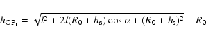
![\begin{displaymath}{\rm H_0P_0}=R_0 \left [\tan \varphi - \frac{\sin \alpha}{\co...
...\varphi}{\cos \varphi} -\frac{h_{\rm s}}{R_0}\right)
\right ]
\end{displaymath}](/articles/aa/full/2006/31/aa4992-06/img101.gif)
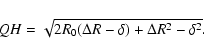
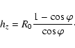
Table A.1:
Height of lower boundary of Earth's shadow at
zenith (hz) and at 60![]() from zenith along the solar meridian
in the Sun's direction.
from zenith along the solar meridian
in the Sun's direction.
![\begin{figure}
\par\includegraphics[width=7.4cm,clip]{4992fg13.eps}
\end{figure}](/articles/aa/full/2006/31/aa4992-06/img115.gif) |
Figure A.2: Normalized density (solid line) and temperature (dashed line) profiles according to the MSIS-E-90 model (Hedin 1991). For comparison, the dots trace the values of the US Standard Atmosphere (McCartney 1976, Table 2.6). |
As anticipated, for the density profile we adopted the MSIS-E-90
model![]() density
profile (Hedin 1991), which is presented in
Fig. A.2. As the plot shows, the global profile can be
roughly described by two laws: one exponential (for h<120 km, the
so-called homosphere) and a power law (for 120<h<400 km, the
so-called thermosphere). Clearly, as the Sun depression increases, the
lower Earth's shadow boundary will pass through more and more tenuous
atmospheric layers and, therefore, the change in density slope should
turn into a change in the twilight sky surface brightness
decline. Under the assumptions made for this simplified model, this
should happen when
density
profile (Hedin 1991), which is presented in
Fig. A.2. As the plot shows, the global profile can be
roughly described by two laws: one exponential (for h<120 km, the
so-called homosphere) and a power law (for 120<h<400 km, the
so-called thermosphere). Clearly, as the Sun depression increases, the
lower Earth's shadow boundary will pass through more and more tenuous
atmospheric layers and, therefore, the change in density slope should
turn into a change in the twilight sky surface brightness
decline. Under the assumptions made for this simplified model, this
should happen when
![]() ,
i.e. close to the end
of nautical twilight.
,
i.e. close to the end
of nautical twilight.
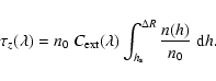
Since in the following section we are interested in the product
between the number density and the extinction cross section, we can
derive this for a given passband by assuming the measured extinction
coefficient
![]() (in mag airmass-1) and integrating
the previous density profile along the vertical (i.e. at airmass 1). In fact, assuming that all the extinction comes from Rayleigh
scattering, one can write:
(in mag airmass-1) and integrating
the previous density profile along the vertical (i.e. at airmass 1). In fact, assuming that all the extinction comes from Rayleigh
scattering, one can write:
The
![]() wavelength dependency of the Rayleigh scattering
cross section is implicitly taken into account by the extinction
coefficients, which are to be considered as input data to the model
and not as free parameters. As for the scattering phase function we
used the canonical expression for air molecules (McCartney
1976):
wavelength dependency of the Rayleigh scattering
cross section is implicitly taken into account by the extinction
coefficients, which are to be considered as input data to the model
and not as free parameters. As for the scattering phase function we
used the canonical expression for air molecules (McCartney
1976):
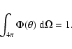
![\begin{displaymath}\Phi(\theta) = \frac{3}{16\pi} \left[1+0.9324\cos^2~(\theta)\right]
\end{displaymath}](/articles/aa/full/2006/31/aa4992-06/img122.gif)
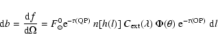
The scattered flux can be computed in the same way as done, for
example, by Krisciunas & Schaefer (1991) for the Moon light. If ![]() is the luminosity of the sun at a given wavelength
(expressed in photons per unit time and per unit wavelength), the flux
received by the Earth at the top of the atmosphere is
is the luminosity of the sun at a given wavelength
(expressed in photons per unit time and per unit wavelength), the flux
received by the Earth at the top of the atmosphere is
![]() ,
where d=1 AU. If we now consider an infinitesimal
volume element dV placed along the line of sight at a distance lfrom O, the number of scattered photons received by the observer per
unit time, unit area, and unit wavelength is given by
,
where d=1 AU. If we now consider an infinitesimal
volume element dV placed along the line of sight at a distance lfrom O, the number of scattered photons received by the observer per
unit time, unit area, and unit wavelength is given by
![\begin{displaymath}{\rm d}f = F_\odot^0 {\rm e}^{-\tau({\rm QP})}\; n[h(l)] \; C...
...ac{\Phi(\theta)}{l^2}\; {\rm e}^{-\tau ({\rm OP})}\;{\rm d}V .
\end{displaymath}](/articles/aa/full/2006/31/aa4992-06/img125.gif) |
(A.4) |

Acknowledgements
We wish to thank S.L. Kenyon and J.W.V. Storey for inspiring this work and the ESO Archive Group for the support received during the data retrieval. O. Ugolnikov is supported by a Russian Science Support Foundation grant. Our gratitude also goes to the referee, Dr. A. Tokovinin, for his useful suggestions and comments.
This paper is based on observations made with ESO Telescopes at Paranal Observatory.