A&A 453, 943-947 (2006)
DOI: 10.1051/0004-6361:20054736
M. V. F. Copetti
Laboratório de Análise Numérica e Astrofísica, Departamento de Matemática, Universidade Federal de Santa Maria, 97119-900 Santa Maria, RS, Brazil
Received 20 December 2005 / Accepted 24 February 2006
Abstract
Context. The spatial electron temperature fluctuations in ionized nebulae that were initially proposed to explain the discrepancies among temperatures obtained from different sensors have been pointed to as the cause of huge inconsistencies among abundances of heavy elements calculated from recombination and forbidden emission lines. Recently, there have been some attempts of direct detection and quantification of spatial temperature fluctuations with point-to-point temperature measurements across the nebula.
Aims. In this paper, we assess the feasibility of estimating the temperature fluctuation parameter t2, the total variance of the spatial distribution of temperature relative to the mean, from the distribution of temperatures measured on the plane of the sky with different sensors.
Methods. Point-to-point measurements of the electron temperature at a series of contiguous and equally spaced rectangular apertures along a radius of homogeneous and spherically symmetric nebulae were numerically simulated for six different temperature sensors.
Results. Variances of projected temperature distributions were obtained and compared with total t2 for different values for the density, ionization parameter and temperature of the ionizing star. The projected profiles of electron temperature obtained from indicators associated with ions occurring at large fractions of the nebula, such as [O III] (
![]() ,
[Ar III]
,
[Ar III]
![]() ,
and the Balmer jump
,
and the Balmer jump
![]() /H
/H![]() ,
are good tracers of the internal gradient of temperature. The variances
,
are good tracers of the internal gradient of temperature. The variances
![]() of the projected temperature distributions measured from these sensors correspond to significant fractions of the total temperature variance, for typical nebulae of the order of
of the projected temperature distributions measured from these sensors correspond to significant fractions of the total temperature variance, for typical nebulae of the order of
![]() 30%, 25%, and 15% for the Balmer jump and the [O III] and [Ar III] ratios, in that order. On the other hand, the temperature profiles obtained from sensors corresponding to low ionization ions, such as [N II] (
30%, 25%, and 15% for the Balmer jump and the [O III] and [Ar III] ratios, in that order. On the other hand, the temperature profiles obtained from sensors corresponding to low ionization ions, such as [N II] (
![]() ,
[O I]
,
[O I]
![]() ,
and [C I]
,
and [C I]
![]() ,
are almost constant at the values of temperature of the outer parts of the nebula, fail to reproduce the true temperature gradient, and have a
,
are almost constant at the values of temperature of the outer parts of the nebula, fail to reproduce the true temperature gradient, and have a
![]() that is always less than 10% and is usually around 1-3% of t2.
that is always less than 10% and is usually around 1-3% of t2.
Key words: ISM: H II regions - ISM: planetary nebulae: general
The theory of photoionized nebulae very successfully explains most of the features observed in the spectra of H II regions and planetary nebulae. This fact has supported the intensive use of these objects as probes of the chemical composition of galaxies. Traditionally, the abundances of heavy elements in ionized nebulae have been obtained from their strong, collisionally excited emission lines. The recent developments in astronomical instruments have made the determination of the abundances of the C, N, and O elements from their weak recombination lines possible. However, huge discrepancies between the abundances obtained from collisionally excited and recombination lines have been found, which cast doubt on the accuracy of the abundance determinations in gaseous nebulae. For example, Liu et al. (1995) determined abundances of C, N, and O in the planetary nebula NGC 7009 by recombination lines and found that they are about 5 times higher than those derived from forbidden lines.
The existence of spatial temperature fluctuations in the nebulae has been suggested as one of the most probable explanations of the inconsistency among abundances calculated from forbidden and recombination lines (Peimbert et al. 1995). Originally, large temperature fluctuations had been proposed by Peimbert (1967) to explain the discrepancies between the values of electron temperature obtained from different indicators.
The magnitude of the temperature fluctuations are usually quantified by the
parameter t2 defined by Peimbert (1967) as
 |
(2) |
However, the magnitudes of the temperature fluctuations needed to reconcile the
recombination line metallicities with those based on collisionally excited lines
or the electron temperature measurements from different line ratios of
planetary nebulae and H II regions of the order
![]() (Luridiana et al. 1999; Esteban et al. 1999b,1998; Peimbert et al. 1995; Esteban et al. 1999a; Dinerstein et al. 1985; Gonzalez-Delgado et al. 1994; Liu & Danziger 1993) are considerably higher than those predicted by
standard photoionisation models (Pérez 1997; Kingdon & Ferland 1995; Gruenwald & Viegas 1995), which
are typically in the range of
(Luridiana et al. 1999; Esteban et al. 1999b,1998; Peimbert et al. 1995; Esteban et al. 1999a; Dinerstein et al. 1985; Gonzalez-Delgado et al. 1994; Liu & Danziger 1993) are considerably higher than those predicted by
standard photoionisation models (Pérez 1997; Kingdon & Ferland 1995; Gruenwald & Viegas 1995), which
are typically in the range of
![]() .
Besides, the physical mechanisms
that could possibly explain the large temperature fluctuations presumed are
unknown. Recently, an alternative solution to the abundance problem has been
proposed and supported based on the assumption of the presence of
hydrogen-deficient and very cold clumps inside the nebula, which, even if they
were to make up only a few percent of the total mass, would be largely
responsible for the emission of recombination lines of heavy elements
(Liu et al. 2000; Tsamis et al. 2004; Tsamis & Péquignot 2005). So, the question of the existence of
substantial spatial variations of electron temperature in nebulae has became a
key issue in the study of H II regions and planetary nebulae.
.
Besides, the physical mechanisms
that could possibly explain the large temperature fluctuations presumed are
unknown. Recently, an alternative solution to the abundance problem has been
proposed and supported based on the assumption of the presence of
hydrogen-deficient and very cold clumps inside the nebula, which, even if they
were to make up only a few percent of the total mass, would be largely
responsible for the emission of recombination lines of heavy elements
(Liu et al. 2000; Tsamis et al. 2004; Tsamis & Péquignot 2005). So, the question of the existence of
substantial spatial variations of electron temperature in nebulae has became a
key issue in the study of H II regions and planetary nebulae.
There have been some attempts of estimating the magnitude of the temperature
fluctuations from point-to-point measurements of the temperature in planetary
nebulae and H II regions (Krabbe & Copetti 2002; Rubin et al. 2002; O'Dell et al. 2003; Liu 1998; Rubin et al. 2003). As a direct estimator for t2, Liu (1998) has proposed the use of
Table 1: Electron temperature indicators and symbols.
We have numerically simulated a point-to-point measurement of the electron
temperature at a series of contiguous and equally spaced rectangular apertures
along the radius of a homogeneous and spherically symmetric nebula. Six
different electron temperature sensors were considered, including the most
commonly used [O III]
![]() ,
[N II]
,
[N II]
![]() ,
and the Balmer jump at 3646 Å relative to H
,
and the Balmer jump at 3646 Å relative to H![]() (see Table 1 for the complete list and for the symbols used for the derived temperatures). The photoionization code
Cloudy 95.03 (Ferland et al. 1998) was used to calculate the thermal and ionization
structure of the nebula. An inner radius of 10% of the outer nebular radius was
assumed. The non-LTE CoStar stellar atmosphere models (Schaerer et al. 1996a; Schaerer & Koter 1997; Schaerer et al. 1996b) for zero age main sequence stars were used. The solar
chemical composition was adopted. We ran models with the effective temperature
of the ionizing star varying from 38 500 to 50 000 K, corresponding to
spectral type from O8 to O3, according to the calibration of Vacca et al. (1996), an
with an ionization parameter in the range
(see Table 1 for the complete list and for the symbols used for the derived temperatures). The photoionization code
Cloudy 95.03 (Ferland et al. 1998) was used to calculate the thermal and ionization
structure of the nebula. An inner radius of 10% of the outer nebular radius was
assumed. The non-LTE CoStar stellar atmosphere models (Schaerer et al. 1996a; Schaerer & Koter 1997; Schaerer et al. 1996b) for zero age main sequence stars were used. The solar
chemical composition was adopted. We ran models with the effective temperature
of the ionizing star varying from 38 500 to 50 000 K, corresponding to
spectral type from O8 to O3, according to the calibration of Vacca et al. (1996), an
with an ionization parameter in the range
![]() and a
hydrogen density
and a
hydrogen density
![]() .
Also, to test
the effects of spatial resolution on the simulations, we varied the number of
apertures in the range
.
Also, to test
the effects of spatial resolution on the simulations, we varied the number of
apertures in the range
![]() .
.
The emissivities of the emission lines involved were calculated with an
n-level atom programme (
![]() )
that we wrote using the atomic
parameters from the IRAF/STSDAS 3.0/nebular package database. For the
fainter lines (e.g. [O III]
)
that we wrote using the atomic
parameters from the IRAF/STSDAS 3.0/nebular package database. For the
fainter lines (e.g. [O III]
![]() or [N II]
or [N II]
![]() ), we considered the contributions to the emissivities due to recombination
and charge transfer effects, since they are significant at some parts of the
nebula. The emissivity of the Balmer jump was calculated from
), we considered the contributions to the emissivities due to recombination
and charge transfer effects, since they are significant at some parts of the
nebula. The emissivity of the Balmer jump was calculated from ![]() (in K units) and the H
(in K units) and the H![]() emissivity predicted by the code Cloudy by the
expression
emissivity predicted by the code Cloudy by the
expression
In Fig. 1, the comparison between the true electron temperature
radial gradient and the spatial profiles of temperature obtained from different
sensors is shown for a typical example of the simulations described in Sect. 2. This figure shows that the temperature indicators can be divided
into two groups. The electron temperature profiles derived from indicators
associated with ions occurring at large fractions of the nebula, such as ![]() (Bac),
(Bac), ![]() (O III), and
(O III), and ![]() (Ar III),
tend to follow the true internal temperature variation fairly well. On the other
hand, the spatial profiles of temperatures obtained from line ratios of low
ionization ions,
(Ar III),
tend to follow the true internal temperature variation fairly well. On the other
hand, the spatial profiles of temperatures obtained from line ratios of low
ionization ions, ![]() (N II),
(N II), ![]() (O I), and
(O I), and ![]() (C I), are almost constant, at values representative of the
higher temperatures predicted for the outskirts of the nebula, and badly fail to
reproduce the inner part of the electron temperature gradient, essentially
because the low ionization ions are concentrated in the outer and hotter parts
of the nebula.
(C I), are almost constant, at values representative of the
higher temperatures predicted for the outskirts of the nebula, and badly fail to
reproduce the inner part of the electron temperature gradient, essentially
because the low ionization ions are concentrated in the outer and hotter parts
of the nebula.
Using expression (3), we calculated the relative variance
![]() of the temperature profile for each temperature sensor considered, then compared
them with the value of t2. The level of dependency of
of the temperature profile for each temperature sensor considered, then compared
them with the value of t2. The level of dependency of
![]() on the
number of apertures N is summarised in Table 2, which shows the range
of the percentage values of
on the
number of apertures N is summarised in Table 2, which shows the range
of the percentage values of
![]() for N = 5, 10, and 20, relative
to
for N = 5, 10, and 20, relative
to
![]() for N = 100, found in the simulations. We verified that
for N = 100, found in the simulations. We verified that
![]() calculated from
calculated from ![]() (Bac),
(Bac), ![]() (O III),
and
(O III),
and ![]() (Ar III) are little dependent on the number of apertures,
especially for
(Ar III) are little dependent on the number of apertures,
especially for ![]() .
Even for as a small number as N = 5, these sensors
produce reasonable results, with
.
Even for as a small number as N = 5, these sensors
produce reasonable results, with
![]() at least 60% of the value for N = 100. This is a consequence of the fact that the photoionization models
predict a fairly smooth gradient of temperature with steep spatial variations
only at the outer border of the nebula (see Fig. 1).
at least 60% of the value for N = 100. This is a consequence of the fact that the photoionization models
predict a fairly smooth gradient of temperature with steep spatial variations
only at the outer border of the nebula (see Fig. 1).
![\begin{figure}
\par\includegraphics[width=7.8cm,clip]{4736fg01.eps}
\end{figure}](/articles/aa/full/2006/27/aa4736-05/img37.gif) |
Figure 1:
Comparison between the true electron temperature radial gradient (solid
line) and the "observed'' spatial profiles of temperature obtained from different
sensors with a very large number of apertures, N = 1000 (broken lines), and
with a small one, N = 20 (marks). The input parameters for this model were:
|
| Open with DEXTER | |
Figures 2 and 3 show the dependence of the electron
temperature fluctuation parameter t2 on the ionization parameter U for a
fixed stellar temperature,
![]() K, and on the effective
temperature of the ionizing star for a fixed ionization parameter,
K, and on the effective
temperature of the ionizing star for a fixed ionization parameter,
![]() ,
and for 6 different values of hydrogen density in the range
,
and for 6 different values of hydrogen density in the range
![]() ,
respectively. These figures illustrate the
kind of relationships between t2, U,
,
respectively. These figures illustrate the
kind of relationships between t2, U,
![]() ,
and
,
and ![]() found
in the complete set of models. The t2 parameter ranges from 0.001 to 0.05,
with little dependency on the stellar effective temperature, but strong
dependency on the hydrogen density for
found
in the complete set of models. The t2 parameter ranges from 0.001 to 0.05,
with little dependency on the stellar effective temperature, but strong
dependency on the hydrogen density for
![]() .
According to the models, denser objects would have more homogeneous temperature
structures, and consequently lower values of t2. The increase of temperature
in the outer parts of the nebula (see Fig. 1), caused by the
hardening of the ionizing radiation as the distance to the centre increases,
which is due to the preferential absorption of low-energy photons in the
photoionization process, is more pronounced in rarefied objects, for which the
ionizations are essentially produced by photons coming directly from the stars.
For denser objects, the much softer diffuse radiation field plays a more
important role in the ionization of the nebula.
.
According to the models, denser objects would have more homogeneous temperature
structures, and consequently lower values of t2. The increase of temperature
in the outer parts of the nebula (see Fig. 1), caused by the
hardening of the ionizing radiation as the distance to the centre increases,
which is due to the preferential absorption of low-energy photons in the
photoionization process, is more pronounced in rarefied objects, for which the
ionizations are essentially produced by photons coming directly from the stars.
For denser objects, the much softer diffuse radiation field plays a more
important role in the ionization of the nebula.
![\begin{figure}
\par\includegraphics[width=7.8cm,clip]{4736fg02.eps}
\end{figure}](/articles/aa/full/2006/27/aa4736-05/img41.gif) |
Figure 2:
Temperature fluctuation parameter t2 vs. the ionization parameter U for
|
| Open with DEXTER | |
![\begin{figure}
\par\includegraphics[width=7.8cm,clip]{4736fg03.eps}
\end{figure}](/articles/aa/full/2006/27/aa4736-05/img42.gif) |
Figure 3:
Temperature fluctuation parameter t2 vs. the effective temperature
|
| Open with DEXTER | |
Table 2:
Dependency of
![]() on the number of apertures N.
on the number of apertures N.
To show the potential use of the present simulations, we have estimated the
global t2 from the measured values of
![]() for 30 Doradus and the Orion Nebulae. From the calibration of the ionization
parameter with the line ratio
for 30 Doradus and the Orion Nebulae. From the calibration of the ionization
parameter with the line ratio
![]() by Diaz et al. (1991), and the
observed line ratios from Kennicutt et al. (2000), we estimate a value of
by Diaz et al. (1991), and the
observed line ratios from Kennicutt et al. (2000), we estimate a value of
![]() for both of these objects. The electron density is
for both of these objects. The electron density is
![]() (Esteban et al. 1998) in the Orion Nebula
and
(Esteban et al. 1998) in the Orion Nebula
and
![]() (Peimbert 2003) in
30 Doradus. The spectral type of the main ionizing stars is O6 or O7 V
in the Orion Nebula (Conti & Alschuler 1971; Copetti & Bica 1983) and O3 in 30 Doradus
(Massey & Hunter 1998), which correspond to
(Peimbert 2003) in
30 Doradus. The spectral type of the main ionizing stars is O6 or O7 V
in the Orion Nebula (Conti & Alschuler 1971; Copetti & Bica 1983) and O3 in 30 Doradus
(Massey & Hunter 1998), which correspond to
![]() K and 50 000 K, respectively, according to the calibration of Vacca et al. (1996). From
Fig. 5, we verify that
K and 50 000 K, respectively, according to the calibration of Vacca et al. (1996). From
Fig. 5, we verify that
![]() is 24% of t2 for the 30 Doradus Nebula and 28% of t2 for the Orion Nebula.
is 24% of t2 for the 30 Doradus Nebula and 28% of t2 for the Orion Nebula.
![\begin{figure}
\par\includegraphics[width=7.8cm,clip]{4736fg04.eps}
\end{figure}](/articles/aa/full/2006/27/aa4736-05/img52.gif) |
Figure 4:
Temperature fluctuation parameter of the simulated measurements of |
| Open with DEXTER | |
![\begin{figure}
\par\includegraphics[width=7.8cm,clip]{4736fg05.eps}
\end{figure}](/articles/aa/full/2006/27/aa4736-05/img53.gif) |
Figure 5:
Temperature fluctuation parameter of the simulated measurements of |
| Open with DEXTER | |
For the Orion Nebula, from the value of
![]() measured by O'Dell et al. (2003), we derive
t2 = 0.028, which is the same value as
that obtained by O'Dell et al. (2003) using a completely different approach. They
evaluated the temperature fluctuation for the whole nebula from the projected
[O III] temperature distribution, based essentially on the fraction of
the nebular volume occupied by the O++ zone and on the difference between
the mean temperatures in the O+ and O++ zones. Through long-slit
spectroscopy, Rubin et al. (2003) have obtained eight independent estimates of
measured by O'Dell et al. (2003), we derive
t2 = 0.028, which is the same value as
that obtained by O'Dell et al. (2003) using a completely different approach. They
evaluated the temperature fluctuation for the whole nebula from the projected
[O III] temperature distribution, based essentially on the fraction of
the nebular volume occupied by the O++ zone and on the difference between
the mean temperatures in the O+ and O++ zones. Through long-slit
spectroscopy, Rubin et al. (2003) have obtained eight independent estimates of
![]() for four different
for four different
![]() areas over the Orion Nebula, finding values from 0.00682 to 0.0176, which
correspond to t2 varying from 0.024 to 0.062, according to our models. The
two highest values for
areas over the Orion Nebula, finding values from 0.00682 to 0.0176, which
correspond to t2 varying from 0.024 to 0.062, according to our models. The
two highest values for
![]() were found for the fainter
areas, consequently from data with poorer S/N. The median of their estimates
from brighter areas,
were found for the fainter
areas, consequently from data with poorer S/N. The median of their estimates
from brighter areas,
![]() ,
is probably more
representative of the whole nebula, and it leads to t2=0.035.
Esteban et al. (1998) estimated
,
is probably more
representative of the whole nebula, and it leads to t2=0.035.
Esteban et al. (1998) estimated
![]() from the comparison of O++ abundances from collisionally excited and recombination lines.
from the comparison of O++ abundances from collisionally excited and recombination lines.
Although a more profound discussion about the existence of significant temperature fluctuations in ionized nebulae is beyond the scope of this paper, we observe that two different conclusions were attained from the above comparisons. For the 30 Doradus Nebula, we estimate a value of t2, compatible with that predicted by photoionization models, but too small to invoke the temperature fluctuations as the cause of the discrepancy between the abundances derived from collisionally excited and recombination lines. On the other hand, for the Orion Nebula, we obtain a magnitude for the temperature fluctuation that could explain the abundance problem, but it is much higher than the predictions of photoionization models for homogeneous nebulae. If the projected temperature variance observed in the Orion Nebula is confirmed (the knotty task is the discount of the pure error variance), it would leave no doubt that the classic temperature fluctuations play an important role in the interpretation of the spectra of H II regions. 2D mapping of temperature with different indicators for a significant sample of objects would be of help to settle the question.
Through model simulations, we have assessed the feasibility of quantifying the global spatial temperature fluctuation parameter t2, based on point-to-point measurements of the electron temperature across the nebula with different temperature sensors. The main conclusions are:
Acknowledgements
This work was partially supported by the Brazilian institutions CNPq and FAPERGS. We thank the anonymous referee for helpful comments and suggestions.
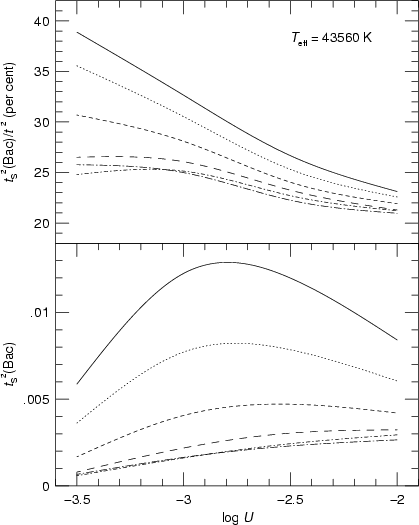 |
Figure 6:
The same as in Fig. 4, except for temperature
|
| Open with DEXTER | |
 |
Figure 7:
The same as in Fig. 5, except for temperature
|
| Open with DEXTER | |
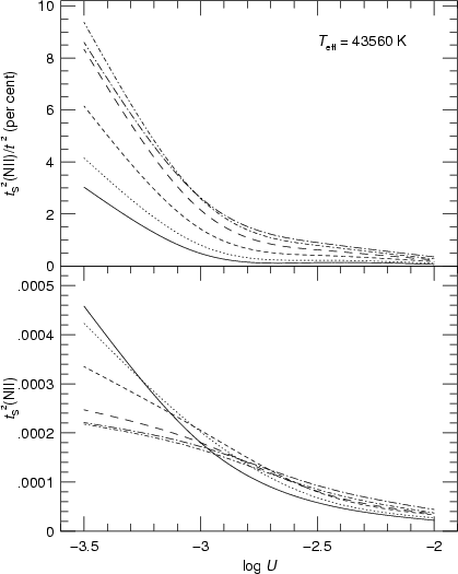 |
Figure 8:
The same as in Fig. 4, except for temperature
|
| Open with DEXTER | |
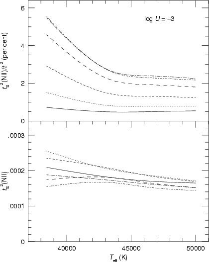 |
Figure 9:
The same as in Fig. 5, except for temperature
|
| Open with DEXTER | |
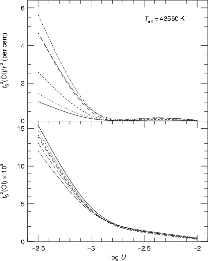 |
Figure 10:
The same as in Fig. 4, except for temperature
|
| Open with DEXTER | |
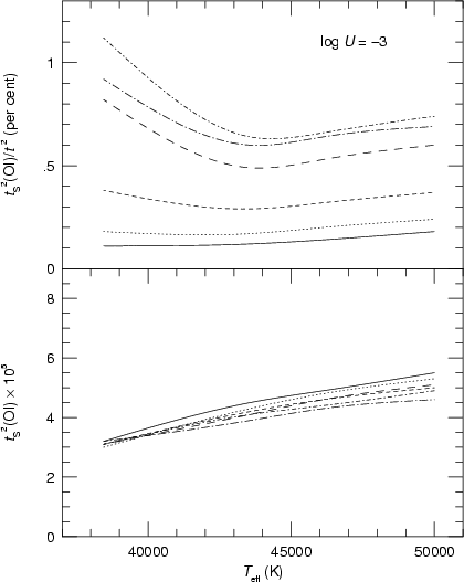 |
Figure 11:
The same as in Fig. 5, except for temperature
|
| Open with DEXTER | |
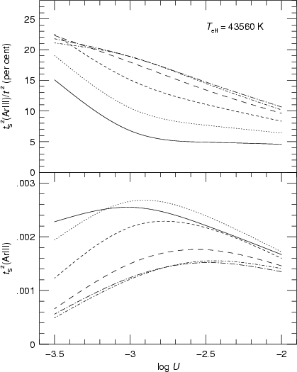 |
Figure 12:
The same as in Fig. 4, except for temperature
|
| Open with DEXTER | |
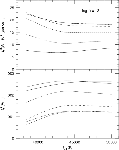 |
Figure 13:
The same as in Fig. 5, except for temperature
|
| Open with DEXTER | |
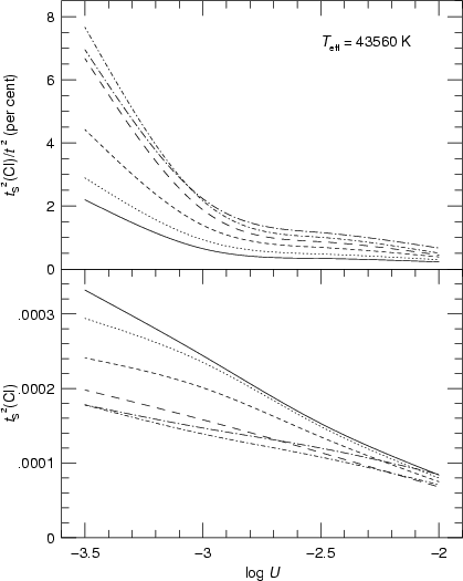 |
Figure 14:
The same as in Fig. 4, except for temperature
|
| Open with DEXTER | |
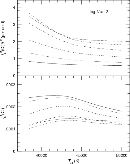 |
Figure 15:
The same as in Fig. 5, except for temperature
|
| Open with DEXTER | |