A&A 452, 321-330 (2006)
DOI: 10.1051/0004-6361:20054285
L. Bettarini1 - S. Landi1 - F. A. Rappazzo2 - M. Velli1,3 - M. Opher3
1 - Department of Astronomy and Space Science, Univ. of Firenze, 50125 Firenze, Italy
2 -
Department of Physics, Univ. of Pisa, 56127 Pisa, Italy
3 -
Jet Propulsion Laboratory, California Institute of Technology, 91109 Pasadena, CA, USA
Received 30 September 2005 / Accepted 9 January 2006
Abstract
We used 2.5D simulations to analyze the magnetohydrodynamic instabilities arising from an initial equilibrium configuration consisting of a plasma jet or wake in the presence of a magnetic field with strong transverse gradients, such as those arising in the solar wind. Our analysis extends previous results by considering both a force-free equilibrium and a pressure-balance condition for a jet in a plasma sheet, along with arbitrary angles between the magnetic field and velocity field. In the force-free case, the jet/wake does not contain a neutral sheet but the field rotates through the flow to invert its polarity. The presence of a magnetic field component aligned with the jet/wake destroys the symmetric nature of the fastest growing modes, leading to asymmetrical wake acceleration (or, equivalently, jet deceleration). In the case of a jet, the instability properties depend both on the magnetic field and flow gradients, as well as on the length of the jet. The results are applied to the post-termination shock jet recently found in 3D global heliospheric simulations, where our analysis confirms and explains the stability properties found in such simulations.
Key words: instabilities - magnetohydrodynamics (MHD) - plasmas - methods: numerical - Sun: solar wind
The evolution of systems consisting of sheared flows in the presence of strong magnetic field gradients is relevant to magnetohydrodynamic (MHD) structures in several solar and astrophysical environments, such as the interaction of the solar wind with a magnetospheric boundary (Uberoi 1984), a model for Earth's magnetotail (Sato & Walker 1982), extragalactic jets (Ferrari 1998), cometary tails (Cravens 1997), galactic center nonthermal filaments (Shore & Larosa 1999) the heliospheric current sheet (hereafter HCS) (Opher et al. 2004; Wang et al. 1988), solar streamers (Einaudi et al. 1999), X-ray jets from the solar corona (Shibata et al. 1992), solar flares (Tsuneta 1996), and more generally, astrophysical jets and wakes (Baty & Keppens 2002; Parhi et al. 1999).
From the first studies of an incompressible plane current-vortex sheet (Dahlburg et al. 1997) and a magnetized jet (Dahlburg et al. 1998), a magnetohydrodynamic model for the formation of the slow solar wind has been developed in which the basic magnetic field is aligned to a fluid wake contained in a neutral sheet (Einaudi et al. 1999). This model accounts for the plasmoid puffs observed in helmet streamers and attributes them to reconnection of the magnetic field at the current sheet, their subsequent acceleration being due to a Kelvin-Helmholtz (hereafter KH) instability triggered once the equilibrium magnetic field is modified by reconnection. In the presence of a magnetic field, the KH instability of a flow parallel to the field lines in an otherwise homogeneous medium sets in, when the velocity jump exceeds the Alfvén speed (Chandrasekhar 1961). The instability criteria are modified in the case of a finite transition (shear) layer and of a compressible medium. This model has been recently improved via the inclusion of compressibility effects (Einaudi et al. 2001), as well as those due to the curvature in a spherical geometry (Rappazzo et al. 2003), while the effect of converging flows has been analyzed by Lapenta & Knoll (2005).
Here we use a 2.5D MHD code to analyze the stability properties and successive evolution of an initially perturbed equilibrium configuration, consisting in a jet flow (or, equivalently, a wake flow) across which there is a change in the initial magnetic field polarity. The angle ![]() between the asymptotic magnetic field (AMF) direction and the jet/wake flow is a free parameter. In our simulations, we scan different values of
between the asymptotic magnetic field (AMF) direction and the jet/wake flow is a free parameter. In our simulations, we scan different values of ![]() to explore how it affects the instability properties, properties which also depend on the relative gradients of magnetic field and velocity through the jet/wake. For example, a one-dimensional field orthogonal to the jet/wake has no influence on the linear stability properties, since perturbations in the plane of the jet/wake do not introduce any magnetic tension. On the other hand, a force-free field configuration (hereafter FFC), where the field "rotates'' across the current sheet, may stabilize the jet/wake if the magnitude is sufficiently strong.
to explore how it affects the instability properties, properties which also depend on the relative gradients of magnetic field and velocity through the jet/wake. For example, a one-dimensional field orthogonal to the jet/wake has no influence on the linear stability properties, since perturbations in the plane of the jet/wake do not introduce any magnetic tension. On the other hand, a force-free field configuration (hereafter FFC), where the field "rotates'' across the current sheet, may stabilize the jet/wake if the magnitude is sufficiently strong.
The primary application of this study is the question of solar wind acceleration above helmet streamers (Woo 1995; Gosling et al. 1981), leading to the slow solar wind streams where one typically observes a global magnetic field polarity inversion, which may or may not coincide with a "neutral sheet''. In a reference frame co-moving with the slow solar wind, we therefore have a bimodal flow profile where the velocity is zero at the HCS, and across it the interplanetary magnetic field (IMF) changes sign from the Southern to the Northern solar hemispheres, regions of fast wind. The magnetic field geometry is shown in Fig. 1, where it reverses direction crossing the wake and has an arbitrary angle ![]() to the flow in the Y-Z plane. Because there are indications (Smith 2001) that the IMF may not vanish through the sheet, but rotates across something like a force-free configuration (FFC) with a finite, though large, plasma
to the flow in the Y-Z plane. Because there are indications (Smith 2001) that the IMF may not vanish through the sheet, but rotates across something like a force-free configuration (FFC) with a finite, though large, plasma ![]() in the HCS, the instabilities of the combined configuration are non-trivial. Depending on the value of
in the HCS, the instabilities of the combined configuration are non-trivial. Depending on the value of ![]() there may also be a stabilizing component of the magnetic field along the shear flow.
there may also be a stabilizing component of the magnetic field along the shear flow.
![\begin{figure}
\par\includegraphics[width=7.4cm,clip]{4285f01.eps}\end{figure}](/articles/aa/full/2006/22/aa4285-05/img10.gif) |
Figure 1: Wind case: reference frame (for v0 and B0 see Eqs. (7)-(9) or (11)-(13)). |
| Open with DEXTER | |
We will consider both an FFC and a simpler model in which the heliospheric current sheet coincides with a neutral sheet and the equilibrium is maintained by a pressure balance condition (PBC). This case also corresponds better to the post-termination shock (hereafter TS) jet that has been recently discovered at the current sheet with 3D numerical simulations by Opher et al. (2003).
This structure was observed to form beyond the solar wind TS on the solar equatorial plane and to extend through the Heliopause (hereafter HP). In the Heliosheath (HS), the region between the TS and the HP, the ![]() parameter decreases by a factor of 103, so the role of the magnetic field is fundamental in that zone. Approaching the TS on the equatorial plane, as schematically shown in Fig. 2, the azimuthal component of the magnetic field downstream the shock is amplified, forming magnetic pressure ridges on either side of the HCS (Suess 1990). Previous numerical studies (Washimi & Tanaka 2001; Linde et al. 1998) have indicated that the HCS also remains in the equatorial plane beyond the TS, so the solar wind can flow freely only in the HCS region, where there is no azimuthal magnetic field that can slow it down. Moreover, the flow undergoes an acceleration due to a de Laval Nozzle process (Opher et al. 2003). This structure is unstable, probably due to the velocity difference between the flow in the current sheet and the surrounding medium.
parameter decreases by a factor of 103, so the role of the magnetic field is fundamental in that zone. Approaching the TS on the equatorial plane, as schematically shown in Fig. 2, the azimuthal component of the magnetic field downstream the shock is amplified, forming magnetic pressure ridges on either side of the HCS (Suess 1990). Previous numerical studies (Washimi & Tanaka 2001; Linde et al. 1998) have indicated that the HCS also remains in the equatorial plane beyond the TS, so the solar wind can flow freely only in the HCS region, where there is no azimuthal magnetic field that can slow it down. Moreover, the flow undergoes an acceleration due to a de Laval Nozzle process (Opher et al. 2003). This structure is unstable, probably due to the velocity difference between the flow in the current sheet and the surrounding medium.
![\begin{figure}
\par\includegraphics[width=7.3cm,clip]{4285f02.eps}\end{figure}](/articles/aa/full/2006/22/aa4285-05/img11.gif) |
Figure 2: Jet case: schematic reconstruction of the heliospheric environment at the TS on the equatorial plane. The magnetic field azimuthal component is amplified across the shock. |
| Open with DEXTER | |
In the following sections we are going to describe the numerical setup for our analysis, the basic conditions, and the chosen initial perturbations, (Sect. 2). In Sect. 3 we summarize the results of the numerical simulations for the FFC and PBC case applied to the wake model of the solar wind, showing that in both cases the evolution depends on whether the basic flow and the AMF are orthogonal or whether there is a generic inclination between them. In Sect. 4 we analyze the numerical results for the heliospheric jet evolution and study its linear instability, comparing several basic configurations. Based on preliminary results concerning the effect of a dipole tilt (Opher 2005, private communication), we consider how this might affect the stability of the jet. In the conclusions Sect. 5, we summarize the results and point to open questions.
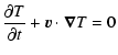
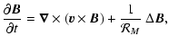
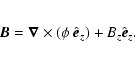
We solve the set of dissipative MHD equations in a Cartesian geometry (see Fig. 1). Analogous with hydrodynamic problems, we define a stream-wise, or Fourier, direction (Y) along which we impose periodic boundary conditions and use spectral methods to calculate derivatives, a cross-stream direction (X) along which the mean flow varies and we impose nonreflecting boundary conditions using the method of the projected characteristics (Vanajakshi et al. 1989; Jeffrey 1969; Roe & Balsara 1996), adopting a compact finite-difference scheme (Lele 1992) coupled with a hyperbolic tangent mesh stretching around the current sheet, and a span-wise direction (Z), corresponding to an invariance direction for the quantities describing our system. Our basic set of equations, written in non-dimensional form, is:
 |
|||
 |
(5) | ||
 |
(6) |
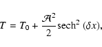
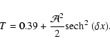
As stated in the introduction, we adopt two different equilibrium configurations. The FFC case is described by the following choice of functions:
In several astrophysical environments the thickness of the neutral sheet is much less than for the shear, such as in the case of the interaction between a galactic magnetized wind and a molecular cloud (Shore & Larosa 1999), as well as in the case of cometary tails (Slavin et al. 1986). At 1 AU from the Sun the HCS has a width of about
![]() km (
km (![]() 6.7
6.7 ![]() 10-5 AU), while the surrounding plasma sheet is thicker by a factor of 30 (Smith 2001): the parameter
10-5 AU), while the surrounding plasma sheet is thicker by a factor of 30 (Smith 2001): the parameter ![]() is much greater than one and it is reasonable to assume that this value remains high near the cusp of the helmet streamers that extend to about
is much greater than one and it is reasonable to assume that this value remains high near the cusp of the helmet streamers that extend to about
![]() from the Sun. In particular we assume that
from the Sun. In particular we assume that
![]() .
Beyond the cusp on the equatorial plane,
.
Beyond the cusp on the equatorial plane,
![]() ,
the simple assumption of mass conservation in a spherically symmetric isothermal atmosphere with radial magnetic field leads to an Alfvén speed that varies between
,
the simple assumption of mass conservation in a spherically symmetric isothermal atmosphere with radial magnetic field leads to an Alfvén speed that varies between
![]() and
and
![]() depending on the assumed values of the density and magnetic field at the base of the coronal region (Mann et al. 2003; An et al. 1990). Fast streams have a velocity of approximately
depending on the assumed values of the density and magnetic field at the base of the coronal region (Mann et al. 2003; An et al. 1990). Fast streams have a velocity of approximately
![]() ,
so the Alfvénic number,
,
so the Alfvénic number,
![]() ,
varies between 1.25 and 2.5. In the simulations shown here we adopt
,
varies between 1.25 and 2.5. In the simulations shown here we adopt
![]() and
and
![]() .
.
Due to numerical constraints we use a value of ![]() smaller than was supposed for the HCS at a few solar radii, however linear and nonlinear theory in the limit of
smaller than was supposed for the HCS at a few solar radii, however linear and nonlinear theory in the limit of
![]() for an incompressible flow (Dahlburg et al. 1998) has shown that the dynamics of the jet/wake configuration is magnetically dominated for
for an incompressible flow (Dahlburg et al. 1998) has shown that the dynamics of the jet/wake configuration is magnetically dominated for
![]() and
and
![]() .
Although the differential velocity between fast and slow streams is supersonic,
.
Although the differential velocity between fast and slow streams is supersonic,
![]() ,
our numerical scheme does not allow us to use such high values. Numerical simulations with different values of the sound Mach number in the range 0.5-1.5 have not shown significant changes in the evolution of the system, so we chose to show here only simulations using the critical value
,
our numerical scheme does not allow us to use such high values. Numerical simulations with different values of the sound Mach number in the range 0.5-1.5 have not shown significant changes in the evolution of the system, so we chose to show here only simulations using the critical value
![]() .
.
For the stability analysis of the heliospheric jet, we use a set of initial parameters obtained from the data reported in Opher et al. (2003):
| (15) | |||
| (16) | |||
| (17) |
Two different initial perturbations are chosen to trigger the instabilities, depending on the equilibrium. For the solar wind case, there are no indications of which instability dominates the linear and nonlinear dynamic of the system and, in particular, which modes drive its evolution according to the direction of the asymptotic magnetic field to the jet/wake flow. We therefore consider a white noise in velocity and in the magnetic potential in order to observe the growth of all the possible unstable modes:
Table 1: Tables of parameters for the solar wind simulations. The last two rows of each table report the maximum linear growth rate for each run and the associated perturbation wave number.
![\begin{figure}
\par\includegraphics[width=5.9cm,clip]{4285f03.eps}\hspace*{2mm}
...
...05.eps}\hspace*{2mm}
\includegraphics[width=5.9cm,clip]{4285f06.eps}\end{figure}](/articles/aa/full/2006/22/aa4285-05/img94.gif) |
Figure 3: Contour of density at different instants for run F0 (see Table 1). |
| Open with DEXTER | |
For
![]() ,
the maximum growth rate of the KH instability and the tearing mode is known to be about 0.35 and 1.35, respectively (Rappazzo et al. 2005). After a few simulations the fundamental wave number,
,
the maximum growth rate of the KH instability and the tearing mode is known to be about 0.35 and 1.35, respectively (Rappazzo et al. 2005). After a few simulations the fundamental wave number,
![]() ,
has been chosen in order to resolve the instability region for each value of
,
has been chosen in order to resolve the instability region for each value of ![]() (see Table 1).
(see Table 1).
For the heliospheric jet we make use of monochromatic incompressible fluctuations as perturbations. From a dynamical point of view, these fluctuations enable the fastest growing instability by neglecting the initial ignition of compressible modes that deprive instability of energy and slow it down. We choose a functional form that rapidly goes to zero at the boundary of the numerical domain in the cross-stream direction. In order not to force the system to evolve according to an instability path that doesn't correspond to the maximum growth rate allowed by the system, the chosen functions must not have a defined parity. One of the possible sets of perturbations that satisfy all the previous constraints is the following:
As in the previous case, the length of the numerical box in the stream-wise direction is adapted to the wave number, i.e.
![]() .
In the cross-stream direction the box length in dimensionless units is
Lx = 23.62, and we use a numerical grid with
.
In the cross-stream direction the box length in dimensionless units is
Lx = 23.62, and we use a numerical grid with
![]()
![]() 128. After several simulations, we decided to assume a value for the Reynolds number such that it is possible to obtain an effective dissipation of energy at the discretization scale, so we consider
128. After several simulations, we decided to assume a value for the Reynolds number such that it is possible to obtain an effective dissipation of energy at the discretization scale, so we consider
![]() .
Actually, their values are much less than their estimations in astrophysical environments, yet they are large enough to assure an ideal dynamic on large scales.
.
Actually, their values are much less than their estimations in astrophysical environments, yet they are large enough to assure an ideal dynamic on large scales.
In Table 1 all performed simulations and characteristic parameters are summarized. Different values of ![]() are considered to study how the relative configuration between the basic magnetic and the sheared velocity field affects the stability properties of the system.
In both F0 and P0 (F and P refer to the FFC and PBC cases, respectively) a Kelvin-Helmholtz sinuous evolution develops, as seen in Fig. 3, where the contour of density at different instants is reproduced for run F0. By computing the average in the cross-stream direction of the Fourier transform (hereafter "1d'' average) of the magnetic potential
are considered to study how the relative configuration between the basic magnetic and the sheared velocity field affects the stability properties of the system.
In both F0 and P0 (F and P refer to the FFC and PBC cases, respectively) a Kelvin-Helmholtz sinuous evolution develops, as seen in Fig. 3, where the contour of density at different instants is reproduced for run F0. By computing the average in the cross-stream direction of the Fourier transform (hereafter "1d'' average) of the magnetic potential
For the PBC case, we observe that the maximum growth rate is almost equal to the one in the other configuration, but the dispersion relation of the unstable modes is significantly shifted towards higher wavenumber values; in particular, the wave number corresponding to the highest growth rate is
![]() .
In the FFC, the magnetic tension of the stream-wise component can inhibit the growth rate at higher wavenumbers. In fact, in the linear regime it is given by
.
In the FFC, the magnetic tension of the stream-wise component can inhibit the growth rate at higher wavenumbers. In fact, in the linear regime it is given by
| (26) |
![\begin{figure}
\par\includegraphics[width=7.65cm,clip]{4285f07.eps}\end{figure}](/articles/aa/full/2006/22/aa4285-05/img111.gif) |
Figure 4:
Average in the cross-stream direction of the Fourier transform of the magnetic potential,
|
| Open with DEXTER | |
Despite the value of
![]() for both FFC and PBC, the evolution of the system is driven by a tearing mode that produces a varicose-resistive instability. Although the precise features of the dynamic depend on the initial configuration of the wake flow and the magnetic field, the nonlinear regime is always characterized by a reconnection process that leads to the destruction of the neutral/current sheet by producing magnetic islands that coalesce afterwards. In Fig. 5 we show the magnetic potential at different instants for run F2: at the end of the linear regime, t = 80, the most unstable modes are well-developed. During the nonlinear regime, the coalescence mechanism leads the system to be structured on larger and larger scales untill the maximum characteristic length allowed by the system is reached. Rappazzo et al. (2005) have studied the evolution of the solar wind FFC wake model using a monochromatic perturbation and considering a magnetic field strictly parallel to the wake, and found a maximum growth rate
for both FFC and PBC, the evolution of the system is driven by a tearing mode that produces a varicose-resistive instability. Although the precise features of the dynamic depend on the initial configuration of the wake flow and the magnetic field, the nonlinear regime is always characterized by a reconnection process that leads to the destruction of the neutral/current sheet by producing magnetic islands that coalesce afterwards. In Fig. 5 we show the magnetic potential at different instants for run F2: at the end of the linear regime, t = 80, the most unstable modes are well-developed. During the nonlinear regime, the coalescence mechanism leads the system to be structured on larger and larger scales untill the maximum characteristic length allowed by the system is reached. Rappazzo et al. (2005) have studied the evolution of the solar wind FFC wake model using a monochromatic perturbation and considering a magnetic field strictly parallel to the wake, and found a maximum growth rate
![]() with an associated wave number
with an associated wave number
![]() .
In Fig. 6 we report the
.
In Fig. 6 we report the ![]() as function of
as function of ![]() ;
the growth rate increases with
;
the growth rate increases with ![]() ,
but as seen in Table 1 the wave number associated with the maximum growth rate increases slightly with
,
but as seen in Table 1 the wave number associated with the maximum growth rate increases slightly with ![]() ,
from
,
from
![]() in F1 to
in F1 to
![]() in F4. Meanwhile, in the PBC it is not affected by the value of the angle between the basic flow and the AMF,
in F4. Meanwhile, in the PBC it is not affected by the value of the angle between the basic flow and the AMF,
![]() ,
although we obtain a rather flat dispersion relation for the different initial configurations. Besides, the PBC linear growth rate is always slightly less than the FFC one. In the run F4 we recover both the same
,
although we obtain a rather flat dispersion relation for the different initial configurations. Besides, the PBC linear growth rate is always slightly less than the FFC one. In the run F4 we recover both the same ![]() and
and
![]() as found by Rappazzo et al. 2005.
as found by Rappazzo et al. 2005.
![\begin{figure}
\par\includegraphics[width=5.9cm,clip]{4285f08.eps}\hspace*{2mm}
...
...10.eps}\hspace*{2mm}
\includegraphics[width=5.9cm,clip]{4285f11.eps}\end{figure}](/articles/aa/full/2006/22/aa4285-05/img116.gif) |
Figure 5: Contour of the magnetic potential field at different instants for run F2 (see Table 1). |
| Open with DEXTER | |
Although FFC and PBC have a very similar linear regime, they show different behavior in the nonlinear regime, when the wake (jet) is accelerated (decelerated). In Fig. 7 we show the cross-stream average of the stream-wise velocity component for different simulations, both in the FFC and PBC case. The Profiles shown are at different instants starting from when the nonlinear regime sets in and the initial condition (solid line) has been plotted as a reference. While for the P-runs the profile is exactly symmetric with respect the stream-wise direction, an asymmetric deceleration of the jet in F-runs is observed. This effect is more relevant for
![]() (first column), and it subsides as its value increases (middle and right column). This reflects the initial parity property of the basic configuration: in the FFC we always have a stream-wise, magnetic field component that produces an anti-symmetric magnetic field with respect to the initial flow: the greater the value of
(first column), and it subsides as its value increases (middle and right column). This reflects the initial parity property of the basic configuration: in the FFC we always have a stream-wise, magnetic field component that produces an anti-symmetric magnetic field with respect to the initial flow: the greater the value of ![]() ,
the lower this asymmetry, and it vanishes for
,
the lower this asymmetry, and it vanishes for
![]() as derived from Eqs. (8), (9). Both in the FFC and PBC, we have an enlargement of the velocity profile, together with a strong jet deceleration which is about
as derived from Eqs. (8), (9). Both in the FFC and PBC, we have an enlargement of the velocity profile, together with a strong jet deceleration which is about
![]() .
This means an acceleration of the solar wind wake such that we can estimate a velocity of about
.
This means an acceleration of the solar wind wake such that we can estimate a velocity of about
![]() for the slow component of the solar wind.
for the slow component of the solar wind.
![\begin{figure}
\par\includegraphics[width=7.7cm,clip]{4285f12.eps}\end{figure}](/articles/aa/full/2006/22/aa4285-05/img121.gif) |
Figure 6:
Wind case: linear growth rate, |
| Open with DEXTER | |
![\begin{figure}
\par\includegraphics[width=5.4cm,clip]{4285f13.eps}\hspace*{2mm}
...
...17.eps}\hspace*{2mm}
\includegraphics[width=5.4cm,clip]{4285f18.eps}\end{figure}](/articles/aa/full/2006/22/aa4285-05/img123.gif) |
Figure 7:
Cross-stream average of the stream-wise velocity component,
|
| Open with DEXTER | |
Table 2: Table of the simulations and parameters for the heliospheric jet. With the label D0 we gather all the monochromatic simulations used to determine the dispersion relation and the linear dynamic features of the heliospheric jet.
![\begin{figure}
\par\includegraphics[width=7.7cm,clip]{4285f19.eps}\end{figure}](/articles/aa/full/2006/22/aa4285-05/img129.gif) |
Figure 8: Dispersion relation given by the simulations summarized in Table 2. The maximum of the curve with the solid line corresponds to the coordinates (0.55, 0.173). |
| Open with DEXTER | |
![\begin{figure}
\par\includegraphics[width=5.9cm,clip]{4285f20.eps}\hspace*{2mm}
...
...22.eps}\hspace*{2mm}
\includegraphics[width=5.9cm,clip]{4285f23.eps}\end{figure}](/articles/aa/full/2006/22/aa4285-05/img130.gif) |
Figure 9: Density contour for run D2 (see Table 2) at different times. The evolution of the system leads inevitably to the destruction of the basic flow in the nonlinear regime. |
| Open with DEXTER | |
Our first set of simulations was performed with the monochromatic incompressible fluctuations given by Eqs. (22), (23), whose wave number was varied in the range
0.15-0.95 as summarized in Table 2. The resulting dispersion relation is shown in Fig. 8 (solid line). It is possible to observe a maximum in the linear growth rate
![]() corresponding to a perturbation wave number
corresponding to a perturbation wave number
![]() .
Taking the characteristic time,
.
Taking the characteristic time,
![]()
![]() 10-2 year, into account, along with the length scale,
10-2 year, into account, along with the length scale,
![]() AU (see Sect. 2), we have a physical growth rate
AU (see Sect. 2), we have a physical growth rate
![]() with a perturbation wave length
with a perturbation wave length
![]() AU.
AU.
For comparison we calculate the linear KH growth rate for an infinitely thin layer in the presence of a uniform magnetic field (Chandrasekhar 1961) that is, in dimensionless units,
![]() ,
where
,
where ![]() is the direction of the wavevector (here
is the direction of the wavevector (here ![]() ),
), ![]() the magnetic field direction, and
the magnetic field direction, and ![]() the direction of the velocity jump across the shear layer. If we consider the values used in our simulations, we find that
the direction of the velocity jump across the shear layer. If we consider the values used in our simulations, we find that
![]() ,
that is,
,
that is,
![]() .
We have a discrepancy of a factor 3, so to observe how this growth rate is influenced by the jet structure and, above all, by the choice of the aB parameter, we carried out simulations with a different ratio between the jet and the neutral sheet width:
.
We have a discrepancy of a factor 3, so to observe how this growth rate is influenced by the jet structure and, above all, by the choice of the aB parameter, we carried out simulations with a different ratio between the jet and the neutral sheet width:
![]() and 5. In order to determine the corresponding dispersion relations, we considered two simulations (D1WN and D2WN respectively) of the jet using a white noise perturbation, as in the solar wind case, but with
and 5. In order to determine the corresponding dispersion relations, we considered two simulations (D1WN and D2WN respectively) of the jet using a white noise perturbation, as in the solar wind case, but with
![]() and an amplitude of
and an amplitude of
![]() .
Afterwards we performed two other simulations (D1 and D2) with a monochromatic perturbation corresponding to the maximum wave numbers previously obtained.
.
Afterwards we performed two other simulations (D1 and D2) with a monochromatic perturbation corresponding to the maximum wave numbers previously obtained.
In Fig. 8 we show the dispersion relations obtained for these two configuration, D1 (dotted line) and D2 (dashed line), and observe that the linear behavior of the system is not affected by the variation of the ![]() parameter. Also in the nonlinear regime for both configurations, we have the same sinuous evolution typical of the KH instability as in the D0 case, which leads to the destruction of the neutral sheet, as shown in Fig. 9 where the contour of the density taken at different instants for run D2 is shown. On the other hand, the size of the neutral sheet can strongly affect the stability properties of the jet. Assuming that the width of the jet is the same order as its length, the maximum wavelength allowed is
parameter. Also in the nonlinear regime for both configurations, we have the same sinuous evolution typical of the KH instability as in the D0 case, which leads to the destruction of the neutral sheet, as shown in Fig. 9 where the contour of the density taken at different instants for run D2 is shown. On the other hand, the size of the neutral sheet can strongly affect the stability properties of the jet. Assuming that the width of the jet is the same order as its length, the maximum wavelength allowed is ![]() 1, in dimensionless units, and
1, in dimensionless units, and
![]() .
In practice, the minimum wavenumber we considered was
.
In practice, the minimum wavenumber we considered was
![]() ,
meaning that the length of the jet is about two times larger than its width. We performed another simulation, D3WN (see Table 2), in which the Alfvénic number, the sonic number, and the asymptotic temperature (see Sect. 2) were the same as the previous simulations. Moreover, we used
,
meaning that the length of the jet is about two times larger than its width. We performed another simulation, D3WN (see Table 2), in which the Alfvénic number, the sonic number, and the asymptotic temperature (see Sect. 2) were the same as the previous simulations. Moreover, we used
![]() to recover the value obtained by Opher et al. (2004). In this case we used a white noise perturbation, whose amplitude is
to recover the value obtained by Opher et al. (2004). In this case we used a white noise perturbation, whose amplitude is
![]() .
In Fig. 10, on the left, we report the first 6 modes of the "1d'' average of the cross-stream velocity as a function of time, while on the right is shown the quadratic fluctuation of the same quantity, that is:
.
In Fig. 10, on the left, we report the first 6 modes of the "1d'' average of the cross-stream velocity as a function of time, while on the right is shown the quadratic fluctuation of the same quantity, that is:
By observing the evolution of a sheared flow in the presence of a strong magnetic field gradient, we are able to make a few considerations about the dynamic properties of a magnetically dominated fluid system. There it is possible to observe a generic inclination between the velocity and the magnetic field, measured by the angle ![]() ,
such as the wake configuration of the solar wind within the first 15-20 solar radii.
,
such as the wake configuration of the solar wind within the first 15-20 solar radii.
We consider two different configurations, a force-free and a pressure balance initial equilibrium, both characterized by the angle ![]() between the initial fluid jet direction and the asymptotic magnetic field. We observe a similar global evolution of the instability for the solar jet/wake for a fixed value of
between the initial fluid jet direction and the asymptotic magnetic field. We observe a similar global evolution of the instability for the solar jet/wake for a fixed value of ![]() ,
but with quite different dynamical features. Both for FFC and PBC we have a typical Kelvin-Helmholtz sinuous evolution for
,
but with quite different dynamical features. Both for FFC and PBC we have a typical Kelvin-Helmholtz sinuous evolution for
![]() ,
while for
,
while for
![]() a linear tearing mode leads to a varicose-resistive instability that determines the start of a reconnection process that in turn leads to a successive coalescence mechanism that drives the final nonlinear evolution of the system on such large scales and destroys the basic system. The two configurations differ essentially due to presence of a stream-wise component of the magnetic field at the initial instant in the force-free case, which is absent for
a linear tearing mode leads to a varicose-resistive instability that determines the start of a reconnection process that in turn leads to a successive coalescence mechanism that drives the final nonlinear evolution of the system on such large scales and destroys the basic system. The two configurations differ essentially due to presence of a stream-wise component of the magnetic field at the initial instant in the force-free case, which is absent for
![]() and becomes more and more relevant as the angle decreases. This produces a displacement between the two dispersion relations because of the stabilizing effect for the higher modes caused by the magnetic tension due to the stream-wise magnetic field component, even if we observe that
and becomes more and more relevant as the angle decreases. This produces a displacement between the two dispersion relations because of the stabilizing effect for the higher modes caused by the magnetic tension due to the stream-wise magnetic field component, even if we observe that
![]() .
.
![\begin{figure}
\par\mbox{\includegraphics[width=8cm,clip]{4285f24.eps}\includegraphics[width=8cm,clip]{4285f25.eps} }
\end{figure}](/articles/aa/full/2006/22/aa4285-05/img151.gif) |
Figure 10:
Jet case: on the left, the first 6 modes of the cross-stream velocity component (averaged along the cross-stream direction),
|
| Open with DEXTER | |
Furthermore for
![]() and
and ![]() ,
the FFC is intrinsically symmetric with respect to the stream-wise direction, while this system does not have a defined symmetry for
,
the FFC is intrinsically symmetric with respect to the stream-wise direction, while this system does not have a defined symmetry for
![]() .
For the PBC configuration, the system is always symmetric and in correspondence of the jet we always have a neutral point. This initial parity property of the two configurations determines the evolution of the HCS, since in the FFC we have a preferential side for magnetic islands formation and a differential acceleration of the wake even if the effect, of course, decreases with the increasing
.
For the PBC configuration, the system is always symmetric and in correspondence of the jet we always have a neutral point. This initial parity property of the two configurations determines the evolution of the HCS, since in the FFC we have a preferential side for magnetic islands formation and a differential acceleration of the wake even if the effect, of course, decreases with the increasing ![]() .
These results can explain observations of a displacement of the HCS with respect to the plasma sheet (Winterhalter et al. 1994), but this effect is completely absent in the PBC. This evolution of a warped HCS could cause the acceleration not only of the slow component of the solar wind, but also of smaller scale structures, like spicules or prominences originating in the chromosphere. We need to perform detailed 3D simulations to account not only for the triggers of compressive modes, but also for considering all the instability modes of the system: in particular all the modes that are orthogonal to the basic flow that in the FFC case should be the most relevant.
.
These results can explain observations of a displacement of the HCS with respect to the plasma sheet (Winterhalter et al. 1994), but this effect is completely absent in the PBC. This evolution of a warped HCS could cause the acceleration not only of the slow component of the solar wind, but also of smaller scale structures, like spicules or prominences originating in the chromosphere. We need to perform detailed 3D simulations to account not only for the triggers of compressive modes, but also for considering all the instability modes of the system: in particular all the modes that are orthogonal to the basic flow that in the FFC case should be the most relevant.
Our 2D simplified model of the 3D configuration of the heliospheric jet shows a typical Kelvin-Helmholtz sinuous evolution, so starting from the data of Opher et al. (2003), we reproduced the general behavior observed in their MHD simulations. Moreover, we determined the characteristic linear growth rate of the instability and the corresponding wavelength: these results confirm their first assessments of these quantities. The variation of the current sheet size does not produce any effect on the instability evolution of the jet, hence on the behavior of the neutral sheet in the Heliosheath region. On the other hand, an increase in the thickness of the neutral sheet at the TS can have a strong influence on the jet stability property, an effect that could be produced by the tilt of the solar magnetic axis to the rotation one, which wasn't accounted for by the simulations performed by Opher et al. (2004). If we consider that the characteristic time of our system is now about
![]()
![]()
![]() and thus larger than the period of the HCS oscillation, which should be on the order of
and thus larger than the period of the HCS oscillation, which should be on the order of
![]()
![]()
![]() ,
then it is reasonable to assume that at the TS we have a mean effect producing an heliospheric jet structure as large as the one assumed in the basic configuration of D3WN (see Table 2). In fact, despite the difficulties detecting the exact position of the TS, recent observations by Voyager 1 have been interpreted as either a TS crossing (Krimigis et al. 2003) or a close approach to this first boundary of the heliosphere (McDonald et al. 2003). Thus, we can assume that the distance of the TS from the Sun is on the order of 100 AU and, if we consider the angle of the tilt to be about
,
then it is reasonable to assume that at the TS we have a mean effect producing an heliospheric jet structure as large as the one assumed in the basic configuration of D3WN (see Table 2). In fact, despite the difficulties detecting the exact position of the TS, recent observations by Voyager 1 have been interpreted as either a TS crossing (Krimigis et al. 2003) or a close approach to this first boundary of the heliosphere (McDonald et al. 2003). Thus, we can assume that the distance of the TS from the Sun is on the order of 100 AU and, if we consider the angle of the tilt to be about
![]() (Fisk 1996), we can estimate an amplitude of about
(Fisk 1996), we can estimate an amplitude of about
![]() for the neutral sheet at the TS. As in the untilted case, the solar wind should stream freely inside the neutral sheet, and it is reasonable to assume that the width of the jet, aV, is roughly the same as aB. Moreover, even if the HS region is poorly known, there are both theoretical and observational indications (Suess & Nerney 1997; Gurnett et al. 1993) that its length is about 50-60 AU. This dimensional analysis of the solar magnetic tilt seems to confirm the hypothesis of the stabilization of the heliospheric jet and agrees with the first MHD simulations (Opher M., private communication). In order to improve our model, we have to point out that the temperature profile and initial hypothesis of constant density are only rough approximations, and we should consider analytical profiles that fit the results in Opher et al. (2003) more closely and that maintain the condition of constant total pressure.
for the neutral sheet at the TS. As in the untilted case, the solar wind should stream freely inside the neutral sheet, and it is reasonable to assume that the width of the jet, aV, is roughly the same as aB. Moreover, even if the HS region is poorly known, there are both theoretical and observational indications (Suess & Nerney 1997; Gurnett et al. 1993) that its length is about 50-60 AU. This dimensional analysis of the solar magnetic tilt seems to confirm the hypothesis of the stabilization of the heliospheric jet and agrees with the first MHD simulations (Opher M., private communication). In order to improve our model, we have to point out that the temperature profile and initial hypothesis of constant density are only rough approximations, and we should consider analytical profiles that fit the results in Opher et al. (2003) more closely and that maintain the condition of constant total pressure.
To test our model further for the slow solar wind and for the heliospheric jet, we first need to extend our computational studies and techniques and, second, to compare the results with new observations of the regions of interest, that is, the streamer belt and the outer Heliosphere. For the former we have the highest expectations for the future Solar Probe Mission, which will go for the first time as close to the Sun as 3 solar radii. In fact, one of the goals of the mission is to observe the production and expulsion of plasmoids from the active regions, observations that could be compared with the images of outwardly moving blobs already given by SOHO/LASCO (Sheeley et al. 1997). Instead, it is necessary for the latter region to exactly determine the time-dependent behavior of the Termination shock, the effects caused by its curvature near the equatorial plane, and the 3D configuration of the Heliosheath region to obtain a detailed 3D instability analysis. In this way we obtain the constraints and the physical quantities to compare with the measurements provided by space missions like Voyager 1 and 2, which are crossing the TS and moving through the Heliosheath, so they will keep on sending us data untill ![]() 2020. Besides, the IBEX (Interstellar Boundary Explorer) Mission will provide global maps of the global interaction between the solar wind and the interstellar medium. IBEX observations will complement to the detailed single-direction measurements provided by Voyager.
2020. Besides, the IBEX (Interstellar Boundary Explorer) Mission will provide global maps of the global interaction between the solar wind and the interstellar medium. IBEX observations will complement to the detailed single-direction measurements provided by Voyager.
Acknowledgements
We acknowledge financial assistance from the European RT network TOSTISP contract No. HPRN-CT-2001-00310 and from the Italian Ministry of Research contract COFIN No. 2002025872. We would like to thank the IPAM program "The Grand Challenge Problems in Computational Astrophysics'' at UCLA where this work was completed. We would like to thank L. del Zanna for the useful suggestions and discussions. We are also grateful to the anonymous referee for comments and suggestions.
![$\displaystyle \rho \frac{\partial \vec{v}}{\partial t} + \rho \vec{v} \cdot \ve...
...{\nabla}) \vec{B} \right] + \frac{1}{\mathcal R} \vec{\nabla} \cdot \vec{\zeta}$](/articles/aa/full/2006/22/aa4285-05/img13.gif)