A&A 450, 1135-1148 (2006)
DOI: 10.1051/0004-6361:20053777

Rotational periods of T Tauri stars in Taurus-Auriga, south of Taurus-Auriga, and in MBM12^,

C. Broeg ^1,2 - V. Joergens³ - M. Fernández^4,5 - D. Husar⁶ - T. Hearty⁷ - M. Ammler¹ - R. Neuhäuser¹

1 - Astrophysikalisches Institut und Universitäts-Sternwarte, Schillergäßchen 2-3, 07745 Jena, Germany
2 - Max-Planck-Institut für Extraterrestrische Physik, Giessenbachstraße, 85748 Garching, Germany
3 - Sterrewacht Leiden / Leiden Observatory, PO Box 9513, 2300 RA Leiden, The Netherlands
4 - Max-Planck-Institut für Astronomie, Königstuhl 17, 69117 Heidelberg, Germany
5 - Instituto de Astrofísica de Andalucía, CSIC, Apdo. 3004, 18080 Granada, Spain
6 - Bundesdeutsche Arbeitsgemeinschaft für Veränderliche Sterne e.V. (BAV), Munsterdamm 90, 12169 Berlin, Germany
7 - Jet Propulsion Laboratory, California Institute of Technology, 4800 Oak Grove Drive, Pasadena, CA 91109, USA

Received 6 July 2005 / Accepted 16 January 2006

Abstract
Context. The ROSAT All-Sky Survey detected many young objects outside any known star forming region. Their formation is yet unclear.
Aims. In order to improve the knowledge about these X-ray bright objects we aimed at measuring their rotational properties, which are fundamental stellar parameters, and at comparing them to young objects inside molecular clouds.
Methods. We monitored photometric variations of 5 T Tauri stars in MBM12 and of 26 young objects in the Taurus-Auriga molecular cloud and south of it. Among the 26 young objects there are 17 weak-line T Tauri stars, 7 zero age main-sequence stars and 2 of unknown type. In addition, 2 main-sequence K-type stars were observed, and one comparison star turned out to be an eclipsing binary.
Results. We found periodic variations for most of the targets. The measured periods of the T Tauri stars range from 0.57 to 7.4 days. The photometric variation can be ascribed to rotational modulation caused by spots. For a few of the periodic variables, changes of the light curve profile within several weeks are reported. For one star such changes have been observed in data taken two years apart. The exceptions are two eclipsing systems. One so far unknown system - GSC2.2 N3022313162 - shows a light curve with full phase coverage having both primary and secondary minima well resolved. It has an orbital period of 0.59075 days. From our spectroscopic observations we conclude that it is a main sequence star of spectral type F2 $\pm$ 4. We further compared the off-cloud weak-line T Tauri stars to the weak-line T Tauri stars inside the molecular cloud in terms of rotational period distribution. Statistical analysis of the two samples shows that both groups are likely to have the same period distribution.

Key words: stars: rotation - stars: fundamental parameters - stars: starspots - stars: variables: general - stars: pre-main sequence - stars: binaries: eclipsing

1 Introduction

The ROSAT All Sky Survey (RASS, Voges et al. 1999) has detected a large number of T Tauri stars (TTS) in the wide surroundings of nearby star-forming regions such as Taurus (Neuhäuser et al. 1995), Lupus (Wichmann et al. 1997), Chamaeleon (Alcalá et al. 1997), Orion (Alcalá et al. 1996), etc. There is an ongoing debate on the nature of the origin of such stars, because they lie far from well known clouds. If the stars formed in dark clouds, a velocity much higher ($\geq$ $3~{\rm km~s}^{-1}$) than the typically measured average velocity (1-2  ${\rm km~s}^{-1}$) is required to carry the stars to their present locations. There are two alternatives which can explain the origin of these stars: i) ejection from their birth clouds with high velocities, as a result of close gravitational encounters (Sterzik & Durisen 1995); ii) formation in small cloudlets which have dissipated. Both theories have a different impact on the rotation of the stars. If the stars were ejected at velocities of 3-10 km s^-1, the ejection would truncate the accretion disk at radii between 1 and 10 AU (Armitage & Clarke 1997). Due to this disruption, the star is supposed to begin to spin up earlier (because of the lack of magnetic breaking) than it is expected from normal evolution. Consequently it is able to reach smaller values for its rotational period. If the stars were born in cloudlets, two facts could have led to rotational periods longer than those of the previously studied weak-line T Tauri stars (wTTS): the long life of the accretion disk due to the lack of interaction with other matter than the star and, possibly, the very low angular momentum of the pre-collapse cloud (as suggested by the lack of remnant dust).

The spectroscopic measurement of the projected rotational velocity of these stars has the disadvantage, that it is only a lower limit for the rotational velocity due to the unknown inclination. A photometric monitoring, on the other hand, can help if inhomogeneous distributions of temperature on the stellar surface cause rotationally modulated brightness variability. Such inhomogeneous distributions, in the form of cool and hot spots, have been observed on TTS since the 60's (Hoffmeister 1965) and have been used in the last decades to determine the rotational periods of many TTS (e.g., Bouvier et al. 1993a; Lamm et al. 2004; Bouvier et al. 1997; Herbst et al. 2004; Cohen et al. 2004; Bouvier et al. 1995; Allain et al. 1996; Bouvier et al. 1993b). Having color information from two or more filters allows the distinction of spot driven brightness variations from other causes, such as eclipses, flares, and pulsations (e.g. Joergens et al. 2001).

With the aim of studying the ROSAT discovered TTS population south of the Taurus clouds, we have carried out a photometric monitoring campaign. Observations were carried out during three observing runs and in at least two filters. Here we present the resulting rotational period distribution and we compare it to that of TTS located in the Taurus clouds. We also present the results of a photometric monitoring carried out of 5 members of the MBM12 association.

Figure 1: Lithium equivalent widths of the objects in this work are plotted versus the effective temperature in order to determine their evolutionary status. The TTS of this work are represented by black squares, the TTS known before ROSAT by $\times$ (adapted from Neuhäuser et al. 1997). In case of low-resolution spectra, where Lithium and iron lines cannot be separated, upper limits are given. The Pleiades are drawn as small circles (values from Soderblom et al. 1993; García Lopez et al. 1994) together with the upper envelope as a solid line. This line defines the Lithium test. Stars with more Lithium than ZAMS stars of the same spectral type (e.g. Pleiades) are younger than ZAMS, i.e. PMS. The conversion from spectral type to effective temperature of the comparison samples was done following Bessell (1991). Furthermore, the iso-abundance lines are shown as dashed lines (from Pavlenko & Magazzù 1996).

Open with DEXTER

2 The sample

Our sample consists of 34 stars: 5 in MBM12 (3 cTTS, 2 wTTS) and 26 young objects and 3 main sequence stars (MS) in the direction of Taurus-Auriga and south of it. Among the 26 young objects, there are 18 wTTS, 6 zero age main-sequence (ZAMS) stars, and 2 of unknown type which are probably young. One of the MS stars was not part of the original sample, but added later because of its apparent photometric variability. The spatial location of the wTTS in and south of Taurus was used to group the objects in in-TA and off-TA subgroups. For the definition of the off-TA positions on the sky see Magazzù et al. (1997), Fig. 1.

  
3 Observations

Observations were conducted at the 1.23 m telescope of the Calar Alto Observatory (Spain) during two observing runs, named hereafter run I and run II. Further observations were carried out at the Himmelsmoor Private Observatory Hamburg (Germany): run III.

Run I took place in November 8 through 17 in 1998 and 21 objects were observed several times per night, using the Johnson VRI filters. Due to unfavorable weather conditions, there are no data for the third and fifth nights. The telescope was equipped with the detector Tek#7, a 1024 $\times$ 1024 pixel CCD camera. Read out noise (RON) and gain of the used detector were $5~[{\rm e}^-]$ and  $0.8~[{\rm e}^-/{\rm DN}]$, respectively. All objects were observed on 9 consecutive nights in three Johnson filters VRI. Typically there are 11 to 30 measurements in each filter per object. Characteristic exposure times were 10-30 s in I, 20-50 s in R, and 50-300 s in the V filter.

Observations during run II were carried out between December 9 and 23 in 2000. Because of bad weather, data were not taken during the night 8, 14, and 15. The observations of all objects span a period of 13 days. Of the 12 objects monitored in this run, two have been already observed during run I. The telescope was equipped with the detector SITe#2b, a 2K $\times$ 2K CCD camera.We used a 1K $\times$ 1K readout window. RON and gain were $6~[{\rm e}^-]$ and  $2.6~[{\rm e}^-/{\rm DN}]$, respectively. The objects in this run were observed in the Johnson BV filters with exposure times ranging from 10 to 300 s in V and 45 to 400 s in B depending on weather conditions and the brightness of the object. Fewer objects were observed leading to many more measurements per object, better S/N, and much better light curves than in Run I.

The field of view (FOV) of both runs I and II was approximately $14\hbox{$.\mkern-4mu^\prime$ }1$ $\times$  $14\hbox{$.\mkern-4mu^\prime$ }1$.

Photometric observations of some of the targets of run I and run II have been also carried out at the 0.4 m Schmidt-Cassegrain-telescope (f = 2.95 m) of the Himmelsmoor Private Observatory Hamburg (Germany) in 26 nights between September 22, 2000, and January 24, 2001, henceforth called Run III. These observations were performed in white light, i.e. without a filter, and with a high sampling rate. Due to weather conditions not every object was observed in every night. The telescope was equipped with Apogee AP7p, a 0.5K $\times$ 0.5K CCD camera with a back-illuminated SITe SI502 chip and a 16-bit analog-digital converter. RON and gain were typically $7{-}11~[{\rm e}^-]$ and $4{-}5~[{\rm e}^-/{\rm DN}]$, respectively. The typical exposure times were 30 s. The CCD camera was operated by MaxIm software. The FOV was approximately $14\hbox{$.\mkern-4mu^\prime$ }3$ $\times$  $14\hbox{$.\mkern-4mu^\prime$ }3$.

There are always several comparison stars (CS) in every field but different CS were used in Run I and II because of the different orientation of the FOV in the two runs.

For the eclipsing binary GSC2.2 N3022313162 a low-resolution CAFOS spectrum was taken at the 2.2 m telescope of the Calar Alto Observatory (Spain) to check the nature of the object. The spectral range was chosen to include both ${\rm H}\alpha$ and Lithium lines because of the object's proximity to a ROSAT position. The slit was oriented so that it covered both the target and its close neighbor, the wTTS RX J0409.3+1716.

4 Photometry

4.1 Data reduction

For run I and II the data were reduced using the CCDRED package of IRAF. The common photometric reductions were performed: overscan subtraction, bias subtraction, and flat field division using sky flat fields. A dark current correction was not necessary.

The data of Run III were reduced by bias subtraction, sky flat field division and dark image subtraction using MIRA.

The CCD reductions and extraction of the CAFOS spectrum were done using IRAF. No standards were observed since a flux calibration was not needed.

4.2 Instrumental magnitudes

Instrumental magnitudes for run I and II were determined for all objects in the field of view. If possible, this was done with aperture photometry: all counts inside a predefined radius were counted. The sky level is determined inside a source-free concentric ring around each object and subtracted. If this was not possible because of very close companions with overlapping point-spread-functions (PSF), PSF-fitting was done to get the instrumental magnitudes. This was necessary for the objects Lk ${\rm H}\alpha$262/263, RX J0312.8-0414NW/SE, RX J0407.3+0113S/N. For both tasks the IRAF package DAOPHOT was used.

For Run III instrumental magnitudes for most of the brighter objects in the field of view were determined by aperture photometry using the software MIRA. The PSF of the objects was only used to determine the optimal radius of the circular apertures and the surrounding annulus. Usually the inner radius of the annulus for local background determination was larger by 2 pixels compared to the radius of the aperture. For small apertures, a good measurement depends upon correctly accounting for the partial pixel coverage. MIRA properly accounts for this case with an exact partial pixel algorithm.

For estimation of the error values of the measurements, MIRA lists a theoretical or calculated estimate of the 1-sigma error based on the readout noise, gain, exposure time, aperture size, and signal level. Further, an empirical or measured estimate of the 1-sigma error based on the noise measured in the background annulus plus the gain, aperture size, and signal level is computed. From both values, the larger value was taken.

  
4.3 Differential photometry

In order to determine the period of the photometric variability of the objects, only relative brightness variations are relevant. Therefore, differential photometry was performed. It has the great advantage of compensating for changes in atmospheric extinction due to clouds and high fog as long as the changes are uniform over the FOV and independent of wavelength. For a small FOV of  $14\hbox{$.\mkern-4mu^\prime$ }1$ the first assumption can be considered to be valid. The error introduced by assuming wavelength independent extinction depends heavily on the filter used, the temperature difference of the objects and the airmass change of the observations (variations due to clouds are grey, but those due to airmass changes are not, as can be global changes of the extinction behavior of the atmosphere).

We applied a new algorithm for differential photometry (Broeg et al. 2005) in run I and II. It makes no a priori assumptions of the CS but rather determines the degree of constancy recursively from the measurements. Therefore it can handle unknown CS and noisy data better than current techniques. Variable or noisy CS will be weighted down or rejected completely. In a first step, the instrumental errors calculated by the photometry software (in our case IRAF) are considered to be correct (to be precise, the average of all observations for each object is used). All CS are then used to calculate a weighted brightness average taking into account the instrumental errors of each CS. This average is subtracted from the object, giving a first differential magnitude. The same is done for all CS, treating them in the same way as the object and using all remaining CS as reference stars keeping the same weights as with the calculation for the object. After this first step, (differential) magnitudes for all CS are available. By calculating the standard deviation of all (time series of) differential magnitudes of the CS, an empirical error estimator for each CS is available. This estimator can now replace the instrumental errors in the calculation of the weights hence leading to slightly different weights and again slightly different standard deviations for the CS. This procedure is repeated until all values converge to constant values. In a final step, the instrumental errors are adjusted by two parameters until their average resembles the empirical standard deviation for all CS. If this is not possible for some CS, those CS must be intrinsically variable and must be removed from the calculations. Now, the above procedure can be repeated one more time giving relative photometry for the object with well defined error bars for all measurements. For a in-depth discussion of this method together with a detailed error analysis concerning effects due to a non-grey atmosphere see Broeg et al. (2005).

5 Time series analysis

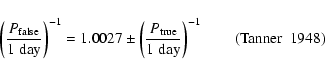
In order to search for periods we mainly used the string-length algorithm, as first proposed by Burke et al. (1970) and discussed in more detail by Dworetsky (1983).

Due to non-random sampling of the data, so-called alias periods are introduced into the signal. For the dominant period, namely one sidereal day, the alias periods can be determined by the well known formula:

$$% \left(\frac{P_{{\rm false}}}{1\; {\rm day}}\right)^{-1}=1.0... ...rm day}}\right)^{-1} \qquad \mbox{\citep{1948JRASC..42..177T}}$$ (1)

which takes into account that objects are observed close to meridian passage. Unfortunately, further sampling effects, i.e. observing the same object every n hours can introduce further, more complicated alias periods.

Because of these difficulties, we used a second, statistical method, based on Monte Carlo simulations to identify the correct period. It takes into account the error bars of the measurements, which are known due to the photometry algorithm (see Sect. 4.3). It generates random light curves of sinusoidal shape with the sampling, amplitude, and errors of the observed data. By doing so, it discovers all alias periods that are produced by the sampling of the data. By comparison of the string-length diagram of real and generated data, the correct period can be determined. This algorithm is described in detail in Broeg et al. (2002) where one of the objects of this study is used as an example.

We did not consider confidence levels since they only give the probability that random noise produces the same period. For all objects there is one or more candidate period where this probability is very low, lower than 1. The drawback with this value is that it gives false confidence in the results: it only says that it is highly unlikely that the signal is just noise, but it does not make any predictions for the alias periods. In some cases two or more periods are equally likely, all have confidence levels above 99.9%, but it is not possible to determine the correct period. In such a case, and when other methods to distinguish between alias and correct period fail, we conclude that no period could be determined.

We accepted a period as correct if the following criteria are fulfilled:

• all filters that allow the determination of a period must arrive at the same period;
• the alias periods (if any) must be clearly identified - either by applying Eq. (1) or by using the Monte Carlo simulation;
• the resulting period must be larger than twice the average sampling time and shorter than the total time of the observing run.

The error bars for the resulting periods represent either the unbiased estimator for the standard deviation of the found periods in the different filters and with the different methods, or the width of the string-length minimum in the string-length algorithm - whichever is larger.

Table 1: Results for all objects. We list all observed objects grouped by membership (MBM12, in-cloud (in TA), off-cloud Taurus-Auriga (off TA), or Orion) and sorted in order of ascending right ascension. The object name is the most common one used in literature - in one case the Guide Star Catalog number was used. The second column gives the observing run in which the object was observed. The calculated period together with the 1$\sigma$ error is given in the next column followed by periods as determined by other groups. In the next five columns, $v \sin i$ values from literature, the spectral type, the classification of the object (w: wTTS,c: cTTS,Z: ZAMS, MS: main sequence, ?: unknown) together with the relevant quantities for the lithium-test ( $W_{\lambda }({\rm Li})$, $W_{\lambda }({\rm H}\alpha )$) are given. Negative values stand for emission, f means the absorption lines are partially filled by emission. The last columns give comments on the nature of the object where relevant (SB1/2: single/double-lined spectroscopic binary). For all values, the sources are given as footnotes at the bottom of the table.

6 Results

   
6.1 General

In this section, the rotational periods for objects of all runs are presented. In difficult cases, or if the object is special in some way, a small paragraph explains the details. The results for all objects are summarized in Table 1. It lists the rotational periods if determined, the classification, and some spectral information for all objects.

In the first observation run, Run I, variation in the brightness could be detected for most objects. If no period could be detected, this was with one exception due to the relatively sparse sampling of the data.

As stated in Sect. 3, all objects of Run II were observed much more frequently than those in Run I. This was probably the reason why variation could be detected and a period could be determined for all objects in this run. The determined periods are therefore very reliable.

The phase folded light curves of the objects for which a period could be determined are shown in Figs. 3-11 for Run I and Figs. 6-9 for Run II. Only the V band results are plotted in the images to conserve space. The V band was chosen because it was used in both runs. For the observations in the other filters see the Online Appendix, Figs. A.1-A.5.

The nature of the variation could be identified as (cold or hot) surface spots by the change in amplitude for different wavelength bands. For spots, the amplitude of the variation increases towards shorter wavelengths, i.e. from the I to the V filter. This was observed in all cases. Only sometimes, the very large noise in the I filter would mimic a larger variation than in the R band when looking at the peak to peak variation. See the data tables (Tables A.1 and A.2) where all important summary data is given for Runs I and II: for each object the noise of the averaged CS was compared to the object's standard deviation and absolute amplitude. This is a suitable way to compare the signal with the noise. In this manner the results for all objects are characterized, and additionally the derived period, number of data points available, total time-span covered, and the range in air-masses is printed. The same information for Run III is shown in Table A.3 but no color and noise information is available there.

For the two eclipsing binaries, we have combined all available photometric measurements, i.e. for GSC2.2 N3022313162 the data from run II and run III and for RX J0408.2+1956 the data from all three runs were combined as shown in Fig. 12. This was done by adding an offset to the instrumental magnitudes. The scaling was untouched. This is only a rough estimate, since the amplitudes of an eclipsing light curve will vary with wavelength if the primary and secondary component are of different spectral type, which is the most likely situation. Otherwise the primary and secondary minima would be of similar depth.

The periods as determined from run III data are consistent with the results from run I and run II for all objects (RX J0406.8+2541, RX J0408.2+1956, RX J0409.3+1716, GSC2.2 N3022313162, RX J0447.9+2755, RX J0452.8+1621, RX J0455.8+1742). The resulting light curves of the TTS are shown in Fig. 13. The zero points of the magnitude scale have been chosen so that the magnitudes correspond roughly to the R-band apparent magnitudes. The given typical error in the lower left corner corresponds to the error of the differential magnitudes, only.

   
6.2 Evolutionary status

Most of the stars had been originally detected by the RASS due to their conspicuous X-ray hardness ratio and classified as pre-main-sequence (PMS) candidates. In follow-up observations, their spectral type and Lithium abundance were determined to verify this classification (see Neuhäuser et al. 1997; Wichmann et al. 1996; Magazzù et al. 1997; Wichmann et al. 2000; Martín & Magazzù 1999; Alcalá et al. 1996,2000; Hearty et al. 2000b). For most of them, their PMS nature could be confirmed.

In order to determine the evolutionary status of the objects, we use the Lithium equivalent width $W_{\lambda }({\rm Li})$, because Lithium is depleted at the early stages of star formation (Neuhäuser et al. 1997). It is our major criterion because of its higher accuracy in the measurable quantities when compared to the second method: placing the objects in the Hertzsprung-Russell Diagram (HRD) and comparing them with theoretical pre-main-sequence tracks, for which the distance is needed (but unknown).

6.2.1 Age from Lithium test

Since stars deplete their Lithium differently for different spectral types, we compared the Lithium abundance to stars of the same spectral type that have just reached the ZAMS: the Pleiades.

The results for all objects in this sample are shown in Fig. 1. They all have more Lithium than the corresponding Pleiades stars. The final classification of the objects can be found in Table 1 together with the results of this study.

   
6.2.2 Age from Hertzsprung-Russell Diagram (HRD)

We also tried to verify the ages of the objects by placing them in the HRD and comparing them with theoretical evolutionary tracks. Since standard stars were only observed in run I, we had to rely on literature values for the absolute brightnesses of all objects in run II, which have relatively large errors.

The next step is correction for interstellar extinction. We use E(R-I) and where 2MASS data are available we supplement it with those data because we think that those bands are least affected by IR- and UV-excesses (see Voshchinnikov & Ilin 1987; Luhman 2001). For the color conversion from spectral type we used Kenyon & Hartmann (1995) for early spectral types and Leggett (1992) for spectral types M0 and later. Masses and ages are interpolated from D'Antona & Mazzitelli (1994).

The distance to the Taurus-Auriga molecular cloud is generally agreed to be around 140 pc (Elias 1978). Concerning the distance to the objects in MBM12, there have been many distance estimates in the past (see Luhman 2001; Hearty et al. 2000a; Andersson et al. 2002; Hobbs et al. 1986; Straizys et al. 2002). For this paper we assume a distance of 90 pc, the shortest of the suggested distances. Enlarging the distance would only make the objects brighter, thus younger. All our MBM12 stars are, using a very small distance of 90 pc and therefore probably overestimating their age, younger than ZAMS.

For each of the studied TTS, the relevant stellar parameters from literature have been compiled in Table A.4. The resulting positions in the HRD relative to PMS tracks and isochrones by D'Antona & Mazzitelli (1994) are shown in Fig. 2. Most objects are confirmed to be young by the ages inferred from the HRD and a few might have already reached the main sequence, whereas some of the objects classified as ZAMS by the Lithium test, might still be younger.

Since the equivalent widths of the Lithium line can be determined quite precisely, and since the errors in the HRD method are larger (especially due to the unknown color excesses), we decided to keep the classification of the Lithium test.

Figure 2: Hertzsprung-Russell diagram with PMS tracks and isochrones. Models are by D'Antona & Mazzitelli (1994). Over-plotted are all weak-line TTS (+) and classical TTS ($\ast$) studied in this paper. Typical error bars are given in the lower left corner. The distance of the Taurus-Auriga objects was assumed to be 140 pc (Elias 1978), for the MBM12 objects a distance of 90 pc (see text) was used.

Open with DEXTER

6.3 Information on selected targets: MBM12

Figure 3: Phase folded light curves: the MBM12 objects in run I for which a period could be determined. For each object only Johnson V is plotted for two orbital phases. All values are given in relative magnitudes $\Delta V$ with arbitrary zero point. The objects' name and period (in days) are printed above each graph. Each data point is given a symbol corresponding to the observation interval it belongs to: when for example plotting a period of 2 days, data points from the first 2 nights will be drawn as plus(+), nights 3 and 4 as asterisk($\ast$), nights 5 through 6 as diamond, followed by filled diamond, triangle, filled triangle, square, filled square, X, circle, and finally if more than 10 phases are present, filled circles are printed for all remaining intervals.

Open with DEXTER

6.3.1 RX J0255.4+2005

Herbst et al. (2004) give the rotational period as 6.22 days, our derived period is 3.36 days - close to half the period determined by the other group. As Herbst et al. (2004) have only one data point per night for each object, their Nyquist frequency prevents them from detecting periods shorter than 2 days and 3.36 days is less than twice that number so this will be difficult to discover. In our data, the 6 day period is also present but it gives a much weaker signal and shows an obvious double maximum in the folded light curve. So we can be sure that 3.36 days is the correct period.

6.3.2 LkH${\alpha }$262

This object shows the strongest variation among the targets of the sample. The period is determined to be P = 1.27 $\pm$ 0.02 days. The star is clearly classified as a young cTTS by its strong ${\rm H}\alpha$ emission and Lithium absorption. The strong variability can be attributed to hot spots on the surface of the accreting star. This interpretation is supported by the amplitude decrease from the V to the I filter. The point that deviates from the lightcurve at phase 0.25 could be due to a flare, since flares are frequent for cTTS (e.g. Stelzer et al. 2000; Guenther & Ball 1999).

Due to the time sampling, Herbst et al. (2004) were not sensitive to the correct period. Moreover, in our data, the 3.13 day period of Herbst et al. (2004) does not appear at all.

6.3.3 LkH${\alpha }$263

For this late-type cTTS (M 4), Herbst et al. (2004) do not report any period, whereas we found a period of 6.6 days. This could be due to the fact that the amplitude during our observations ($\Delta I$ = 0.22 mag) was twice the value they registered.

6.3.4 LkH${\alpha }$264

This star is a cTTS that shows strong variability both in terms of lines (Gameiro et al. 2002) and continuum light. The period that best fits our observations (7.4 days, amplitude I = 0.45 mag) does not match previous results and this could be interpreted as due to long term variability. Mendoza et al. (1990) monitored the star for 10 nights recording an amplitude of 0.59 mag in the V band, but no periodicity. Fernandez & Eiroa (1996) found two tentative, aliased, periods of 1.67 and 2.60 days for August 1991 (amplitude I = 0.26 mag) and two similar values, 1.74 and 2.33 days, for five nights in August 1992 (amplitude I = 0.18 mag). During the long monitoring carried out by Herbst et al. (2004) in 2001 to 2002 the amplitude was small, too (0.28 mag in the I band). They found a period of 2.603 days with a false alarm probability = 0.007.

Further research on the variability of this star is on progress and it will be published elsewhere (Fernández et al., in preparation).

6.4 Information on selected targets: off-TA

   
6.4.1 RX J0312.8-0414NW and RX J0312.8-0414SE

No period could be determined for these two objects. This was not due to a lack of variability, but was caused by the very poor S/N level achieved. The PSF of these two objects overlapped to a great degree making it difficult to separate the light of the two sources. It turned out that the noise introduced by the PSF fitting was too large to detect a signal. On the level of the achieved accuracy, these objects appear to be constant.

6.4.2 RX J0333.1+1036

This object clearly shows variability. Nevertheless, no period can be determined. The results in the different filters are not coherent. The Monte Carlo simulation suggests a period in the vicinity of 2.1 days. However, this is speculative. With better sampling, though, it should be possible to determine the rotation period in this manner.

6.4.3 RX J0344.8+0359

In this case, the amplitude of variation is only slightly larger than the noise. Only around ten data points were available per filter. Nevertheless, all algorithms lead to the same period in all three filters. We therefore identify the period as P= 1.34 $\pm$ 0.09 days.

6.4.4 RX J0407.3+0113S and RX J0407.3+0113N

As for RX J0312.8-0414, the PSFs of the two stars overlap strongly. The photometric precision is only around 0.2 mag. This is not enough to detect a periodic variability in this case. But in contrast to the binary RX J0312.8-0414NW (Sect. 6.4.1) at least one of the stars appears to be variable. The time-scale of the variation seems to be of the order of 2 days. In order to determine a more precise period, a better photometric precision and sampling rate are required.

6.4.5 RX J0434.3+0226

No variation can be detected here despite the very good sampling. Apperently, this star did not exhibit strong spot activity at the time of observations. According to the classification (see Table 1), the star is at the border to the ZAMS. Its age, or a long rotational period, could be the reason for its low variability.

6.4.6 1RXS J044534.0+120917

This object was not part of the original sample. It was a CS that showed variability. We determined a rotational period of P= 3.35 $\pm$ 0.15 days. As of now, there is no spectral information for this object.

6.4.7 RX J0445.5+1207

A very good S/N could be achieved for the light curve of this object due to the availability of a relatively large number of bright, constant CS. Despite the good quality of the data, the search for periods turned out to be difficult. There are two minima in the light curves which are not equidistant. The increase of the amplitude of the lightcurve as the wavelength decreases, i.e. towards the V band, gives strong evidence for star spots as sources of the variation. The smallest string-length occurs at the trial period of 6.3 days in all filters. Because there is a second minimum in the string-lengths diagram at half the period, it looked at first, as if this would be twice the correct period. But on closer inspection, it turned out that both peaks are of different width, namely 2.7 and 3.6 days. This is reproduced independently in all filters. Therefore the light curve must be caused by two (or more) spots of different size on opposite sides of the star. We conclude that the correct period is P= 6.34 $\pm$ 0.05 days.

6.4.8 RX J0450.0+0151

The period search for this star was made difficult by the occurrence of a flare during the observations. After the removal of the flare data points (the circles around phase $\phi=0.5 / 1.5$ in Fig. 5), the string-length algorithm determined the same period in all filters.

The light curve shows a very steep rise in brightness around the minimum of the light curve. All open circled data points belong to the same interval of observations, i.e. were observed consecutively. This shows that the rise is not an artefact from wrong phase folding, but a true increase in brightness. The plot for the period P= 2.23 $\pm$ 0.03 days is shown in Fig. 5 including the flare data points.

6.4.9 RX J0528.9+1046

This object was first classified as a wTTS but after resolving both components of this double lined spectroscopic binary, the Lithium equivalent width for each component was reduced to less than 300 mÅ, the threshold value for spectral type K. So we now classify this star as ZAMS. Furthermore, Torres et al. (2002) conclude that this object is member of $\lambda$-Ori, so does not belong to the Taurus-Auriga group. See Fig. 5 for the V light curve of this star.

6.4.10 RX J0529.3+1210

This wTTS has been observed in both runs, but only few measurements are available. Surprisingly, with only 8 data points in each filter in run II, only a period of 2.14 and its alias period of 0.68 days show a minimum in the string-length algorithm. Because the amplitude has changed from run I to run II, it is not possible to combine the data sets. Nevertheless, the rotational period as determined from the two runs is consistent and we give the period as P= 2.14 $\pm$ 0.20 days. The resulting light curves are printed in Figs. 5 and 9.

6.5 Information on selected targets: in-TA

	Figure 4: Phase folded light curves: all Taurus-Auriga objects in run I for which a period could be determined (Part I). Explanation see Fig. 3.
Open with DEXTER

	Figure 5: Phase folded light curves: all Taurus-Auriga objects in run I for which a period could be determined (Part II). Explanation see Fig. 3.
Open with DEXTER

	Figure 6: Phase folded light curves: the objects in run II for which a period could be determined (Part I). Symbol conventions are the same as in Fig. 3.
Open with DEXTER

	Figure 7: Phase folded light curves: the objects in run II for which a period could be determined (Part II). Symbol conventions are the same as in Fig. 3.
Open with DEXTER

	Figure 8: Phase folded light curves: the objects in run II for which a period could be determined (Part III). Symbol conventions are the same as in Fig. 3.
Open with DEXTER

	Figure 9: Phase folded light curves: the objects in run II for which a period could be determined (Part IV). Symbol conventions are the same as in Fig. 3.
Open with DEXTER

6.5.1 RX J0406.8+2541

This object's amplitude of brightness variation is 0.29 mag in the V-band, the largest amplitude of all the wTTS in our sample. It also has ${\rm H}\alpha$ emission suggesting that there is large activity.

The period search was difficult despite the large variation. The reason for this was a flare in the observation and a change in the spot pattern on the time-scale of one rotation. This can be seen in Fig. 6: consecutive intervals do not overlap according to the error bars for the found period of 1.7 days. This effect is most prominent around phase $\Phi=0.6$ in the V band. This shows that a change in the spot pattern or temperature of the spots must have occured on short time-scales. It shall be noted that the prominent deviating data points in the V-band correspond to a revolution of the star where no corresponding B-band images were taken (black triangles). The open square data point (in Fig. A.5), however, has a corresponding simultaneous observation in the V-band which is weaker in amplitude, as should be the case for flares. All flare candidate data points are situated away from the maximum brightness of the star, as is expected for flares correlated to active regions. Furthermore it has been shown that flaring activity can be connected to changes in the spot distribution (see Fernández et al. 2004, for a detailed flare analysis of V410 Tau).

It has to be noted that a period of twice the length of the found period cannot be ruled out. Bouvier et al. (1997) find also a period of 1.73 days for this object, but they do not have enough data points to make that distinction. We have to admit, though, that twice the period is still a possibility. Keeping in mind that 3.4 days cannot completely be ruled out as period we conclude that the most likely period is P= 1.70 $\pm$ 0.02 days.

This result was independently confirmed in Run III.

6.5.2 RX J0407.9+1750

Because of the poor phase coverage (see Fig. 6), the period of P=0.985 $\pm$ 0.005 days is a tentative period, only.

6.5.3 RX J0408.2+1956

The object RX J0408.2+1956, also known under the name of V1196 Tau, was already known to be an eclipsing binary with a 3.01 day period. The better sampling in run III allows a more precise period determination. It is now constrained to P=3.0109 $\pm$ 0.0002 days. This is the value we give in Table 1. The heliocentric epoch of the minimum is at HJD $_{\rm min}=2~451~818.4579$. The resulting V-band light curves can be inspected in Figs. 4, 7 and a much better light curve from Run III in Fig. 13.

The combined lightcurve from all runs is shown in Fig. 12b. The white light observations of run III can't be expected to fit properly since the amplitude should vary depeding on filter, but both V band data sets should be comparable. So it remains unclear why the data points do not overlap according to the errors.

6.5.4 RX J0409.3+1716

Looking at the phase folded light curve for the period of P= 0.60 $\pm$ 0.01 days in Fig. 7, the scatter in the data points is apparently quite large. On closer inspection, there appears to be a second period overlaid. Fitting two sinusoids to the data gives two periods: 0.6 and 1.8 days. Therefore we give the period as P= 0.60 $\pm$ 0.01 days mentioning that the second component of the spectroscopic binary could have a rotational period of P=1.8 $\pm$ 0.1 days.

6.5.5 GSC2.2 N3022313162

This star was serendipitously in the FOV of the star RX J0409.3+1716 and it was meant to serve as a CS only. During the differential photometry procedure, it became apparent that it is strongly variable. We therefore analyzed the light curve separately. The result is an extremely well sampled light curve of an eclipsing binary system. It is shown in Fig. 7. For this object, the combination of runs II and III did not allow a more precise period determination. The gap in time between run II and III was too large. 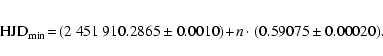The period is determined as P= 0.59075 $\pm$ 0.00020 d and the heliocentric epoch of the minimum brightness is:

$$\begin{eqnarray*}{\rm HJD}_{\rm min}\!=\!(2~451~910.2865 \pm 0.0010)\!+\!n \cdot (0.59075\pm 0.00020). \end{eqnarray*}$$

We took a low-resolution CAFOS spectrum to determine the spectral type of the primary component. The spectra of GSC2.2 N3022313162 and RX J0409.3+1716 were taken simultaneously in one slit with the goal of obtaining more information about the eclipsing object GSC2.2 N3022313162. Both spectra are shown, continuum normalized to 1, in Fig. 10.

	Figure 10: Spectra of the two objects a) GSC2.2 N3022313162 and b) RX J0409.3+1716. The spectral range is 4650 to 8300 Å.
Open with DEXTER

From the spectrum, we determine the spectral type of the primary component of GSC2.2 N3022313162 to be F2 $\pm$ 4. Therefore it is a background object. This object has also been observed in run III where an excellent phase coverage was achieved. The combined run I and III lightcurve is shown in Fig. 12a.

6.5.6 RX J0439.4+3332A

For this object, the second best sampling of the entire campaign was achieved. The variability amplitude of this object is 0.1 mag. The string-length algorithm produces the same period in all filters: 2.42 days. The light curve for this period (see Fig. 8) clearly shows two maxima, which might hint at 1.2 days as the true period. However, at closer inspection, the two maxima are of different amplitude and they are not spaced evenly apart. Therefore we conclude that P= 2.42 $\pm$ 0.02 days is the correct rotational period. However, the signal in the B band is not larger than in the V band in this case. Even though this is most likely caused by the high noise level in the B band, the nature of the signal cannot be unambiguously determined to be spots.

6.5.7 RX J0447.9+2755

This object, like RX J0406.8+2541, seems to exhibit a change in amplitude during the observation. The amplitude increase at the end of the observing run can be seen in Fig. 8 which shows the light curve phase folded with a period of 1.27 days: for observations at later times (X, circles), the amplitude has become larger. This is probably the reason why the string-length for three times the period ($\approx$3.9 days) is smaller in some filters. But since it is very unlikely to have three spots of very similar size spaced evenly apart, we conclude that P= 1.27 $\pm$ 0.02 days is the correct period and that a change in amplitude has taken place during the observations.

	Figure 11: Phase folded light curves: the object in orion (run I). Explanation see Fig. 3.
Open with DEXTER

	Figure 12: Phase folded light curves of the two eclipsing binaries. a) GSC2.2 N3022313162 with data of run II and III. The black squares are the measurements from run II. b) RX J0408.2+1956 with combined data from all three runs. The open diamonds represent data from run I, the open squares run II, and the small crosses are the run III measurements.
Open with DEXTER

	Figure 13: Phase folded light curves: all TTS observed in run III. Values are white light apparent magnitudes. The typical error is given in the lower left corner of each figure.
Open with DEXTER

6.6 Analysis of the distribution of rotational periods

After the presentation of the individual results, we continue with a statistical analysis of the rotational periods.

The distribution of the wTTS south of the Taurus-Auriga molecular cloud (off-TA) is shown in Fig. 14a. It is compared to the in-TA wTTS composed of the wTTS from this study and further wTTS in Taurus-Auriga that have been known before ROSAT (see Table A.5). The period distribution is shown in Fig. 14b. Unfortunately there are only 6 objects remaining in our study for which a period could be determined, which were both located in the southern region and could be confirmed as wTTS.

	Figure 14: Distribution of rotational periods compared: all off-TA wTTS are compared to the in-TA wTTS.
Open with DEXTER

To quantify the differences in the two samples, we computed the Kaplan-Meier Estimators according to Feigelson & Nelson (1985) and Isobe et al. (1986) with the program ASURV (1990). It is plotted in Fig. 15: obviously, both samples are quite similar. Note that we used no data censoring as the unability to determine a period does not represent an upper or lower limit. We only used the stars where a period was determined for the statistical analysis.

In a next step we compared the two samples with two-sample tests. In order to make as few assumptions as possible we used linear rank statistic tests (for a general overview of statistical tests, see Sheskin 2000), namely: Gehan's generalized Wilcoxon Test with permutation variance (1), Gehan's generalized Wilcoxon Test with hyper-geometric variance (2), and the Log-rank Test (3). They are described in detail in Feigelson & Nelson (1985).

We tested for the null hypothesis H₀: F₁ (t) = F₂ (t) that both samples are taken from the same distribution, or more precisely: in the underlying populations represented by the two samples, the median of the difference scores equal to zero. We want to test the non-directional (or two-tailed) null hypothesis to the 0.05 significance level. The results are printed in Table 2. Obviously, the null hypothesis H₀ cannot be rejected but quite the opposite is true: it is highly likely that both samples are drawn from the same distribution (P $\sim$ 80%).

Table 2: Results of the two-sample tests. The tested hypothesis was H₀: F₁ (t) = F₂ (t): both samples are equal. The probability p of H₀ being true is given for the three tests. This shows that the two samples must be considered equal.

   
6.7 Discussion

In order to be able to distinguish between in-situ formation of the TTS in little cloudlets and ejection from the cloud, we have compared the rotational periods of the off-cloud wTTS to the in-cloud wTTS.

In the frame of the magnetospheric accretion model (see Hartmann et al. 1998) the rotational velocity depends strongly on the lifetime of the accretion disk, because the presence of a disk prevents the spin up during contraction due to magnetic breaking (Bouvier et al. 1993a; Edwards et al. 1993). Ejection from the cloud would most certainly disrupt the disk or at least lead to a significantly reduced lifetime of the disk (Armitage & Clarke 1997). Therefore, the off-cloud TTS should rotate faster if they were ejected from the cloud. In-situ formation in small cloudlets, on the other hand, should lead to a prolonged disk lifetime and therefore slower rotation.

As was shown in the previous section, both off-TA and in-TA groups appear to share the same distribution of rotational periods. This is tentative evidence in favour of the in situ formation model as ejected stars should exhibit faster rotation. It must be considered, however, that only 6 objects with a determined rotational period remained in the off-TA sample. For all other objects (10), the PMS nature could not be confirmed, or no period determined. Furthermore, it is well known that there is a dependence of the rotational period on mass and age of the star (theoretical models predict a spin up of the star during the first Myr, see Fig. 5 of Bouvier et al. 1997). Therefore, only subgroups of similar mass and age should be compared for reliable results. Having only 6 objects, this is not possible.

	Figure 15: Kaplan-Meier estimator of the periods of the wTTS: wTTS situated south of the Taurus-Auriga molecular cloud (solid line) compared to the wTTS inside the cloud (dashed line). The distributions are very similar.
Open with DEXTER

We must therefore conclude, that even though the mean rotation period of the two groups under investigation does not differ significantly, we cannot distinguish between the two proposed formation scenarios.

7 Conclusions

In this study, 34 objects, among them 22 TTS, were monitored photometrically in three different observing runs: Run I and II at the 1.23 m telescope of the Calar Alto Observatory in November 1998 (8 nights) and December 2000 (12 nights) and Run III at the Himmelsmoor Private Observatory Hamburg from September 2000 to January 2001 (26 nights). For 15 TTS a period of photometric variability could be determined. It could be identified as rotational variation caused by star spots due to the characteristic dependence of the amplitude on wavelength.

The rotational periods of the TTS in Taurus-Auriga range from 0.57 to 6.34 days.

All five objects in MBM12 exhibited strong photometric variation, so that a clear period of variability could be determined for one wTTS and all three cTTS. The wTTS for which we could not determine a period also showed strong variability but the poor sampling did not permit to distinguish the real from the alias periods. The rotational periods in MBM12 range from 3.36 to 7.4 days.

Furthermore, photometric periods, most likely identified as rotational modulation caused by star spots, could be measured for 5 ZAMS in/near the Taurus-Auriga molecular cloud.

This study added new rotational periods for 10 TTS and 6 ZAMS stars near the Taurus-Auriga molecular cloud, and 4 new periods in MBM12. Another ZAMS period could be confirmed.

Two of the objects, both not PMS stars, show eclipses. For RX J0408.2+1956 this was already known. Its orbital period could be constrained to 3.0109 $\pm$ 0.0002 days. The other one, GSC2.2 N3022313162, shows a very well sampled eclipsing light curve with an orbital period of only 0.59075 $\pm$ 0.00020 days. It was discovered by the algorithm by its unusually large variability that did not fit the error model. Spectroscopic follow-up observations show that it is not a young object but an old background binary of spectral type early F.

When statistically comparing the rotational periods found here for off-cloud wTTS south of Taurus-Auriga with wTTS inside the Taurus-Auriga molecular cloud, there is no significant difference in the period distribution. However, having only 6 off-TA stars, no conclusions in favour of one of the two formation scenarios can be drawn.

Acknowledgements

It is a pleasure to acknowledge fruitful collaborations with the Bundesdeutsche Arbeitsgemeinschaft für Veränderliche Sterne e.V. (BAV, German workgroup for variable stars) which led to the joint observations of professional and amateur astronomers this paper is based on.
C.B. was supported, in part, by the Deutsches Zentrum für Luft- und Raumfahrt (DLR), Förderkennzeichen 50 OW 0205.
V.J. and R.N. did most of this research when they were still at MPE Garching.
V.J. acknowledges support from the Deutsche Forschungsgemeinschaft (Schwerpunktprogramm "Physics of star formation'') and by a Marie Curie Fellowship of the European Community program "Structuring the European Research Area'' under contract number FP6-501875.
M.F. was initially supported, in part, by the Spanish grant AYA2004-05395 and later by the Deutsches Zentrum für Luft- und Raumfahrt (DLR), Förderkennzeichen 50 OR 0401.
We have made use of VizieR, ADS, and the SIMBAD databases.

References

• Alcalá, J. M., Covino, E., Torres, G., et al. 2000, A&A, 353, 186 [NASA ADS]
• Alcalá, J. M., Krautter, J., Covino, E., et al. 1997, A&A, 319 184
• Alcalá, J. M., Terranegra, L., Wichmann, R., et al. 1996, A&AS, 119, 7 [EDP Sciences] [NASA ADS]
• Allain, S., Fernandez, M., Martin, E. L., & Bouvier, J. 1996, A&A, 314, 173 [NASA ADS]
• Andersson, B.-G., Idzi, R., Uomoto, A., et al. 2002, AJ, 124, 2164 [NASA ADS] [CrossRef]
• Armitage, P. J., & Clarke, C. J. 1997, MNRAS, 285, 540 [NASA ADS]
• ASURV. 1990, BAAS, 22, 917 (In the text)
• Bessell, M. S. 1991, AJ, 101, 662 [NASA ADS] [CrossRef]
• Bouvier, J., Bertout, C., Benz, W., & Mayor, M. 1986, A&A, 165, 110 [NASA ADS]
• Bouvier, J., Cabrit, S., Fernandez, M., Martin, E. L., & Matthews, J. M. 1993a, A&AS, 101, 485 [NASA ADS]
• Bouvier, J., Cabrit, S., Fernandez, M., Martin, E. L., & Matthews, J. M. 1993b, A&A, 272, 176 [NASA ADS]
• Bouvier, J., Covino, E., Kovo, O., et al. 1995, A&A, 299, 89 [NASA ADS]
• Bouvier, J., Wichmann, R., Grankin, K., et al. 1997, A&A, 318, 495 [NASA ADS]
• Broeg, C., Fernández, M., & Neuhäuser, R. 2005, Astron. Nachr., 326, 134 [NASA ADS] [CrossRef]
• Broeg, C., Joergens, V., Hearty, T., et al. 2002, in 1st Potsdam Thinkshop on Sunspots and Starspots, ed. K. G. Strassmeier, & A. Washuettl, Brandenburgische Universitätsdruckerei, Golm, 39 (In the text)
• Burke, E. W., Rolland, W. W., & Boy, W. R. 1970, JRASC, 64, 353 [NASA ADS] (In the text)
• Chavarría-K, C., Terranegra, L., Moreno-Corral, M. A., & de Lara, E. 2000, A&AS, 145, 187 [EDP Sciences] [NASA ADS]
• Cohen, R. E., Herbst, W., & Williams, E. C. 2004, AJ, 127, 1602 [NASA ADS] [CrossRef]
• D'Antona, F., & Mazzitelli, I. 1994, ApJS, 90, 467 [NASA ADS] [CrossRef]
• Dworetsky, M. M. 1983, MNRAS, 203, 917 [NASA ADS] (In the text)
• Edwards, S., Strom, S. E., Hartigan, P., et al. 1993, AJ, 106, 372 [NASA ADS] [CrossRef]
• Elias, J. H. 1978, ApJ, 224, 857 [NASA ADS] [CrossRef] (In the text)
• Feigelson, E. D., & Nelson, P. I. 1985, ApJ, 293, 192 [NASA ADS] [CrossRef]
• Fernández, M., Stelzer, B., Henden, A., et al. 2004, A&A, 427, 263 [EDP Sciences] [NASA ADS] [CrossRef]
• Fernandez, M., & Eiroa, C. 1996, A&A, 310, 143 [NASA ADS]
• Gameiro, J. F., Folha, D. F. M., & Costa, V. M. 2002, A&A, 388, 504 [EDP Sciences] [NASA ADS] [CrossRef]
• García Lopez, R. J., Rebolo, R., & Martin, E. L. 1994, A&A, 282, 518 [NASA ADS]
• Grankin, K. N. 1993, Info. Bull. Var. Stars, 3823, 1 [NASA ADS]
• Grankin, K. N., Ibragimov, M. A., Melnikov, S. J., Shevchenko, V. S., & Yakubov, S. D. 1991, Info. Bull. Var. Stars, 3658, 1 [NASA ADS]
• Guenther, E. W., & Ball, M. 1999, A&A, 347, 508 [NASA ADS]
• Hartmann, L., Calvet, N., Gullbring, E., & D'Alessio, P. 1998, ApJ, 495, 385 [NASA ADS] [CrossRef]
• Hearty, T., Fernández, M., Alcalá, J. M., Covino, E., & Neuhäuser, R. 2000a, A&A, 357, 681 [NASA ADS]
• Hearty, T., Neuhäuser, R., Stelzer, B., et al. 2000b, A&A, 353, 1044 [NASA ADS]
• Herbst, W. 1989, AJ, 98, 2268 [NASA ADS] [CrossRef]
• Herbst, W., Williams, E. C., & Hawley, W. P. 2004, AJ, 127, 1594 [NASA ADS] [CrossRef]
• Hobbs, L. M., Blitz, L., & Magnani, L. 1986, ApJ, 306, L109 [NASA ADS] [CrossRef]
• Hoffmeister, C. 1965, Veroeff. Sternw. Sonneb., 6, 97
• Isobe, T., Feigelson, E. D., & Nelson, P. I. 1986, ApJ, 306, 490 [NASA ADS] [CrossRef]
• Joergens, V., Guenther, E., Neuhäuser, R., Fernández, M., & Vijapurkar, J. 2001, A&A, 373, 966 [EDP Sciences] [NASA ADS] [CrossRef]
• Kenyon, S. J., & Hartmann, L. 1995, ApJS, 101, 117 [NASA ADS] [CrossRef]
• Lamm, M. H., Bailer-Jones, C. A. L., Mundt, R., Herbst, W., & Scholz, A. 2004, A&A, 417, 557 [EDP Sciences] [NASA ADS] [CrossRef]
• Leggett, S. K. 1992, ApJS, 82, 351 [NASA ADS] [CrossRef]
• Luhman, K. L. 2001, ApJ, 560, 287 [NASA ADS] [CrossRef]
• Magazzù, A., Martin, E. L., Sterzik, M. F., et al. 1997, A&A, 124, 449 [NASA ADS] (In the text)
• Martín, E. L., & Magazzù, A. 1999, A&A, 342, 173 [NASA ADS]
• Mendoza, E. E., Rolland, A., & Rodriguez, E. 1990, A&AS, 84, 29 [NASA ADS]
• Mora, A., Merín, B., Solano, E., et al. 2001, A&A, 378, 116 [EDP Sciences] [NASA ADS] [CrossRef]
• Neuhäuser, R., Sterzik, M., Torres, G., & Martin, E. 1995, A&A, 299, L13 [NASA ADS] (In the text)
• Neuhäuser, R., Torres, G., Sterzik, M. F., & Randich, S. 1997, A&A, 325, 647 [NASA ADS]
• Ochsenbein, F., Bauer, P., & Marcout, J. 2000, A&AS, 143, 23 [EDP Sciences] [NASA ADS]
• Pavlenko, Y. V., & Magazzù, A. 1996, A&A, 311, 961 [NASA ADS]
• Rydgren, A. E., Zak, D. S., Vrba, F. J., Chugainov, P. F., & Zajtseva, G. V. 1984, AJ, 89, 1015 [NASA ADS] [CrossRef]
• Sheskin, D. J. 2000, Handbook of Parametric on Nonparametric Statistical Procedures, 2nd edn. (CRC Press) (In the text)
• Soderblom, D. R., Jones, B. F., Balachandran, S., et al. 1993, AJ, 106, 1059 [NASA ADS] [CrossRef]
• Stelzer, B., Neuhäuser, R., & Hambaryan, V. 2000, A&A, 356, 949 [NASA ADS]
• Sterzik, M. F., & Durisen, R. H. 1995, A&A, 304, L9 [NASA ADS]
• Straizys, V., Cernis, K., Kazlauskas, A., & Laugalys, V. 2002, Baltic Astron., 11, 231 [NASA ADS]
• Tanner, R. W. 1948, JRASC, 42, 177 [NASA ADS]
• Torres, G., Neuhäuser, R., & Guenther, E. W. 2002, AJ, 123, 1701 [NASA ADS] [CrossRef] (In the text)
• Voges, W., Aschenbach, B., Boller, T., et al. 1999, A&A, 349, 389 [NASA ADS] (In the text)
• Voshchinnikov, N. V., & Ilin, V. B. 1987, Sov. Astron. Lett., 13, 157 [NASA ADS]
• Vrba, F. J., Rydgren, A. E., Chugainov, P. F., Shakovskaia, N. I., & Weaver, W. B. 1989, AJ, 97, 483 [NASA ADS] [CrossRef]
• Wichmann, R., Krautter, J., Covino, E., et al. 1997, A&A, 320, 185 [NASA ADS]
• Wichmann, R., Krautter, J., Schmitt, J. H. M. M., et al. 1996, A&A, 312, 439 [NASA ADS]
• Wichmann, R., Torres, G., Melo, C. H. F., et al. 2000, A&A, 359, 181 [NASA ADS]

 

  
Online Material

   
Appendix A

A.1 Additional data

Table A.1: Measured periods, variability amplitudes, and errors of all objects in Run I. In this table all measurements in the filters  VRI are given. The first column gives the total time span covered by the observations followed by the total airmass range of the observations. The next columns describe the noise in each band. For each filter X, the amplitude of variation  $\Delta m_{\rm X}$, the standard deviation of the object  $\sigma _{\rm X}$, the standard deviation of the averaged comparison star  $\sigma _{\rm X}^{{\rm av.}}$, as well as the number of data points are listed. Hence, the variation of the object can be compared to the noise level of the reference stars. The last column gives the determined period together with the 1$\sigma$-error. The numbers in parentheses refer to some comments in the footnotes.

Table A.2: Measured periods, variability amplitudes, and errors of all objects in Run II. In this table, the results in the filters V and B are given. The information is the same as for Run I in Table A.1.

Table A.3: Measured periods and variability amplitudes in Run III. The second column lists the determined periods with estimated error interval, the last column gives the amplitude of the unfiltered brightness variation in magnitudes. All results are consistent with Run I and II measurements.

Table A.4: Stellar parameters relevant for the Hertzsprung-Russell Diagram of all objects. The objects are grouped by type and sorted by right ascension. For the objects in Taurus, a distance of  $140~{\rm pc}$ is assumed, for MBM12 $90~{\rm pc}$. The color excess that was used to calculate the extinction A_V is given in the neighboring column. To get the real colors of the objects we used the spectral type - color conversion from Kenyon & Hartmann (1995) for early spectral types and Leggett (1992) for type M0 and later. The masses and ages are interpolated from pre main sequence models by D'Antona & Mazzitelli (1994). The apparent magnitudes in V for objects observed in Run I was determined by absolute photometry ourselves. For Run II objects we had to rely on VizieR (Ochsenbein et al. 2000) values - we averaged all available values. For more details see text.

Table A.5: All wTTS in the comparison sample. They have been known prior to the ROSAT All-Sky Survey. The table lists the rotational period together with the classification of the object. All objects are weak-line TTS, wb stands for binarity, wt for triple system, wsb is a double-lined spectroscopic binary. The last column states if the object was detected with the Einstein observatory (marked with X) and is therefore X-ray selected like the stars found by ROSAT.

A.2 Light curves in other filters

Figure A.1: Phase folded light curves: I band light curves of the MBM12 objects in run I for which a period could be determined. Explanation of the symbols see Fig. 3.

Figure A.2: Phase folded light curves: R band light curves of the MBM12 objects in run I for which a period could be determined. Explanation of the symbols see Fig. 3.

Figure A.3: Phase folded light curves: the I band light curves of all Taurus-Auriga objects in run I for which a period could be determined. Explanation see Fig. 3.

Figure A.4: Phase folded light curves: the R band light curves of all Taurus-Auriga objects in run I for which a period could be determined. Explanation see Fig. 3.

Figure A.5: Phase folded light curves: the B band light curves of the objects in run II for which a period could be determined. Symbol conventions are the same as in Fig. 3.