A&A 450, 645-654 (2006)
DOI: 10.1051/0004-6361:20054089

Hydrodynamical simulations of the jet in the symbiotic star MWC 560

II. Simulations beyond density balance

M. Stute

Landessternwarte Heidelberg, Königstuhl, 69117 Heidelberg, Germany

Received 23 August 2005 / Accepted 19 December 2005

Abstract
Context. In the first paper of this series, we presented hydrodynamical simulations with radiative cooling of jet models with parameters representative of the symbiotic system MWC 560. These were jet simulations of a pulsed, initially underdense jet in a high-density ambient medium. They were stopped when the jet reached a length of 50 AU. There, however, a transition of the initially underdense jet towards an overdense jet should occur, which should result in changed kinematics. A few minor differences between the models and the observations were thought to be solved by a model with an increased jet density during the pulses which was calculated only with purely hydrodynamical means in the former paper.
Aims. Therefore, we describe two hydrodynamical simulations with cooling beyond this density balance, one with the same parameters as model i in Paper I (now called model i$^\prime$), which was presented there with and without cooling, and the second with higher gas densities in the jet pulses (model iv$^\prime$).
Methods. Hydrodynamical simulations, with a further approximated cooling treatment compared to Paper I, were used to be able to enlarge the computational domain.
Results. The transition causes changes in the expansion of the cocoon and therefore the morphology of the jet, e.g. a larger radial width of the jet knots. We investigate the radiation properties of the jets, the bremsstrahlung and optical emissivities, integrated emission maps, and synthetic absorption line profiles.
Conclusions. The conclusion that the high observed velocities in CH Cygni, R Aquarii, and MWC 560 favor the models with cooling is unchanged by the transition. The observed parallel features in R Aquarii can be produced by the internal knots or by a variable dense radiative shell of shocked ambient medium. The absorption line profiles show that the real parameters in MWC 560 are closer to model iv$^\prime$ than to model i$^\prime$.

Key words: ISM: jets and outflows - binaries: symbiotic - line: profiles - hydrodynamics - methods: numerical

1 Introduction

The emergence of jets is a very common phenomenon in a variety of astrophysical objects, and it occurs in systems of very different size and mass scales. Jets are observed in active galactic nuclei (AGN) in which they are formed around supermassive black holes, in X-ray binaries with stellar black holes or neutron stars, in young stellar objects (YSO), in supersoft X-ray sources and in symbiotic stars. Symbiotic systems consist of a red giant undergoing strong mass loss and a white dwarf. More than one hundred symbiotic stars are known, but only about ten systems show jet emission. The most famous systems are R Aquarii, CH Cygni, and MWC 560.

R Aquarii, with a distance of about 200 pc, is one of the nearest symbiotic stars and a well known jet source. The jet has been extensively observed in the optical, at radio wavelengths, and with X-ray observations (e.g. Kellogg et al. 2001; Hollis et al. 1985a; Paresce & Hack 1994; Solf & Ulrich 1985; Hollis et al. 1985b). It shows a rich morphology, e.g. a series of parallel features in the jet and the counter-jet, extending a few hundred AU each. In 1984/85 CH Cygni showed a strong radio outburst, during which a double-sided jet with multiple components was ejected (Taylor et al. 1986). This event allowed an accurate measurement of the jet velocity near 1500 km s^-1. In HST observations (Eyres et al. 2002), arcs can be detected that also could be produced by episodic ejection events. While the first two objects are seen at high inclinations, the jet axis in MWC 560 is practically parallel to the line of sight. This special orientation provides an opportunity to observe the outflowing gas as line absorption in the source spectrum. With such observations the radial velocity and the column density of the outflowing jet gas close to the source can be investigated in great detail. In particular we can probe the acceleration and evolution of individual outflow components with spectroscopic monitoring programs, as described in Schmid et al. (2001).

In Stute et al. (2005, hereafter Paper I), we presented hydrodynamical simulations with and without cooling of jets with parameters that were intended to represent those in MWC 560. In a grid of eight simulations we investigated the influence of different jet pulse parameters. Due to the high computational costs of simulations including cooling, this grid was restricted to adiabatic simulations. Only one model simulation was performed that included a treatment of radiative cooling.

The adiabatic jet models showed some quantitative differences for the different pulse parameters. In comparison with the model including cooling, huge differences were present. Those concern, e.g., a significantly higher bow-shock velocity and a well-defined periodic shock structure with high-density, low-temperature knots separated by hot, low-density beam sections in the radiative model. The expansion velocity of CH Cyg was shown to agree very closely with the jet model with cooling. The situation in R Aqr was less clear. The observationally derived proper motion was more in the range of the gas motion of the adiabatic models, although the origin of the observed emission has not been confirmed yet. The small jet opening angle of 15$^{\circ}$ favored a jet with cooling more. We showed that the adiabatic jet models are not able to produce low temperature regions, which are, however, necessary to explain strong absorptions from low ionization species in the spectra of MWC 560 as Ca II, but the cooling of the jet gas still did not seem efficient enough. This should be achieved by another model with higher gas densities in the jet outflow. The basic structure of the observed jet absorptions in MWC 560 was reproduced, including the mean velocity, the velocity width and temporal evolution of the highest velocity components, but not their strengths. Again, another model with higher gas densities should solve this.

A drawback of our former simulations was the fact that they were stopped when the jet reached a length of 50 AU. This is unsatisfactory from an observational point of view, as the observed extents of the jet in R Aquarii and CH Cygni are much larger, as well as from the theoretical viewpoint. At this point, the density of the environment has decreased down to the density in the jet nozzle. A transition of the initially underdense jet towards an overdense jet should occur, which should result in changed kinematics. Underdense jets decelerate more than overdense jets, because the position of the jet head can be basically derived from a balance of the ram pressures of jet and external medium and because the relative importance of ram and thermal pressure should also change. As the kinematics of the models was one of the results of the former models, which were compared with the observations, it should be tested whether simulations with larger spatial scales lead to new insights into the physics of jets in symbiotic stars.

Therefore, we performed two hydrodynamical simulations with cooling beyond this density balance, one with the same parameters as model i in Paper I, which was presented both with and without cooling, and the second with higher gas densities in the jet pulses. Due to constraints set by the available computer resources, we were forced to approximate the former treatment of radiative cooling again.

In Sect. 2, we briefly describe the changes of our model with respect to Paper I. After a validating of the approximated cooling treatment in Sect. 3, we investigate the global and internal structure of the jet (Sect. 4) and its consequences on the emission (Sect. 5.1). Then synthetic absorption line profiles are calculated in Sect. 5.2. Finally a summary and a discussion are given.

   
2 The numerical models

2.1 The computer code

The general capabilities of the code NIRVANA_CP have already been described in detail in Paper I. The code was written by Ziegler & Yorke (1997) and modified by Thiele (2000) to calculate radiative losses due to non-equilibrium cooling by line emission. It solves the equations of ideal hydrodynamics with an additional cooling term in the energy equation $\Lambda ( T ; \rho_{i})$ and a network of rate equations:

 

$$\frac{\partial~\rho}{\partial~t} + \nabla~(\rho~\vec{v})$$ = 0

$$\frac{\partial~(\rho~\vec{v})}{\partial~t} + \nabla~ (\rho~\vec{v}\otimes\vec{v}) - \nabla~p - \rho~\nabla~\Phi$$ =

$$\frac{\partial~e}{\partial~t} + \nabla~(e~\vec{v}) - p~\nabla~\vec{v} + \Lambda ( T ; \rho_{i})$$ =

$$(\gamma - 1)~e$$ p =

$$\frac{\partial~\rho_{i}}{\partial~t} + \nabla~(\rho_{i}~\vec{v}) \sum_{i=1}^{N_{s}}~\sum_{j=1}^{N_{s}}~k_{ij} (T)~\rho_{i}~\rho_{j} .$$ = (1)

Here $\rho$ is the gas density, e the internal energy, $\vec{v}$ the velocity, $\gamma$ the ratio of the specific heats at constant pressure and volume, and $\rho_{i}$ the species densities satisfying $\rho = \sum_{i=1}^{N_{s}}~\rho_{i}$ for the total density. k_ij are the rate coefficients for two-body reactions which are functions of the fluid temperature T. They describe electron collision ionization and radiative and dielectronic recombination processes. When the cooling is solved dynamically with the full set of non-equilibrium equations, the various ionization states and concentration densities $\rho_{i}$ of each element are calculated from the atomic rate equations. They are used explicitly in the cooling functions as

$$\Lambda ( T ; \rho_{i}) = \sum_{i=1}^{N_{s}}~\sum_{j=1}^{N_{s}}~e_{ij} (T)~ \rho_{i}~\rho_{j} + \Lambda_{BS} (T)$$ (2)

with e_ij the cooling rates from two-body reactions between species i and j, and $\Lambda_{BS}$ the cooling function due to Bremsstrahlung.

Table 1: Parameters of the jet pulses: the model number, the density of the pulse in the nozzle $n_{\rm {pulse}}$ in cm^-3, the velocity of the pulse in the nozzle $v_{\rm {pulse}}$ in cm s^-1, the mass outflow during the pulse $\dot M$ in g s^-1 and in ${M}_{\odot }$ yr^-1, and the kinetic jet luminosity during the pulse in erg s^-1.

Due to constraints set by the available computer resources, our former simulation with cooling, presented in Paper I, included a simpler treatment of radiative effects. Instead of the full explicit cooling function $\Lambda ( T ; \rho_{i})$ for all species, we considered only cooling by hydrogen, together with a general non-equilibrium (NEQ) cooling function $\Lambda ( T )$ adapted from Sutherland & Dopita (1993) to account for the cooling by the heavier elements. This cooling function was derived by calculating several atomic processes as electron collision ionization, radiative and dielectronic recombination, line radiation, and Compton heating in the temperature range between 10⁴ and 10^8.5 K. For hydrogen we solved the atomic network of H  I, H  II, and e^- and calculated the cooling due to collisional ionization of H  I and due to collisional excitation of hydrogen line emission.

To perform the simulations beyond density balance with cooling, we were forced to simplify the treatment of cooling again. We neglected the atomic network with its rate equations and used the ionization fractions of hydrogen as a function of temperature given by Sutherland & Dopita (1993), calculated by using the recombination, collisional ionization, and charge transfer rates. We included Bremsstrahlung and the general cooling function calculated with these partial densities. In NEQ models the ionization fraction could be higher than in the case of collisional ionization equilibrium (CIE), due to the slow process of recombination of hydrogenic and helium-like ions. Only at temperatures of about 10⁵ K, however, is the CIE cooling timescale smaller than the equilibration timescale for those ions (Sutherland & Dopita 1993), leading to the difference between the CIE and the NEQ cooling curve used. As hydrogen is (almost) completely ionized at temperatures higher than 20 000 K, the differences in the ionization fractions are almost negligible in the temperature range of the cooling curve. Small differences should only occur in low temperature regions of the jet.

Figure 1: Comparison of temperature ( top), density ( middle), and ionization fraction ( bottom) plots of the old model i ( left) and model i$^\prime$ ( right) at day 74. Besides slight differences in the internal morphology, the dimensions of the jets, positions of the internal shocks, and temperatures are identical in both simulations; differences in the ionization fractions arise in the low-temperature regions of the jet due to the larger equilibration timescales in this temperature range.

Open with DEXTER

Figure 2: $\rho - T$-histogram of eight consecutive days (day 62-69) covering one pulse cycle of model i ( left) and model i$^\prime$ ( right). The bright bar at very low temperatures and at densities between 10-16 and 10-14 g cm-3 consists of the external medium. The internal dense knots build up the line at T = 104 K. The new pulse becomes visible as an arc and spreads out along a line of constant temperature.

Open with DEXTER

	Figure 3: As Fig. 2, continued. The radiative cooling lowers the temperature of the region of higher densities. Superposed on it, the whole feature moves towards lower densities and lower temperatures, consistent with adiabatic expansion. The slope of the path is approximately $\log ( T ) \sim 2 / 3 ~ \log ( \rho )$.
Open with DEXTER

2.2 The parameters

The geometrical model is taken over without changes, except for the dimensions of the computational domain. We choose a two-dimensional slice of the full domain and assume axisymmetry. In these new simulations, the dimension in axial direction is doubled to 100 AU to be able to study the jet propagation after density compensation. The resolution remains unchanged as 20 grid cells per AU (jet beam radius).

The hot component is located in the origin of the coordinate frame, therefore the companion is expanded into a "Red Giant Ring''. In the 2D integration domain, only half of the cross-section of this ring on this slice is included. The binary separation in the models is chosen to 4 AU which is of the order of the estimated separations of 3.3-5.2 AU. The density of the red giant is set to $2.8 \times 10^{-5}$ g cm^-3 and its radius to 1 AU.

Surrounding the red giant, a stellar wind is implemented. The wind has a constant velocity of v=10 km s^-1, a gas temperature of T=50 K, and a mass loss of 10^-6  ${M}_{\odot }$ yr^-1. The density of the red giant wind at the surface of the star is then $2.2 \times 10^{-14}$ g cm^-3. The density of the external medium is given by a $1/r^2_{\rm {rg}}$-law for a spherical wind where $r_{\rm {rg}}$ is the distance from the center of the red giant. The density of the red giant wind near the jet nozzle is about 200 times higher than the initial jet density. At a distance of 50 AU from the symbiotic system, i.e. at the end of the integration domain of the former simulations, the wind density is about equal to the jet density at the nozzle.

To account for the counter-jet and the other part of the jet, respectively, the boundary conditions in the equatorial plane and on the jet axis are set to reflection symmetry. On the other boundaries, outflow conditions are chosen.

The jet is produced within a thin jet nozzle with a radius of 1 AU. The initial velocity of the jet is chosen to 1000 km s^-1 or 0.578 AU d^-1 and its density is set to $8.4 \times 10^{-18}$ g cm^-3 (equal to a hydrogen number density of $5 \times 10^6$ cm^-3). These parameters lead to a density contrast $\eta$ of $5 \times 10^{-3}$, a Mach number of ${\approx} 60$ in the nozzle and a mass loss rate of ${\approx} 10^{-8}$  ${M}_{\odot }$ yr^-1. Repeatedly each seventh day, the velocity and density values in the nozzle are changed to simulate the jet pulses which are seen in the observations of MWC 560.

The pulse parameters of the first simulation were chosen as in the old model i with cooling of Paper I. The nomenclature is now model i$^\prime$ - mention of the cooling will be omitted hereafter. A second simulation with parameters as in the adiabatic model iv - the model with the highest density pulses - was also performed and is now named model iv$^\prime$.

Table 1 lists the main parameters of the models: the model number, the density of the pulse in the nozzle $n_{\rm {pulse}}$ in cm^-3, the velocity of the pulse in the nozzle $v_{\rm {pulse}}$ in cm s^-1, the mass loss during the pulse $\dot M$ in g s^-1 and in  ${M}_{\odot }$ yr^-1, and the kinetic jet luminosity during the pulse in erg s^-1. Each pulse lasts for one day.

   
3 Validating the cooling treatment

By the aforementioned simplifications of the cooling treatment, we achieved a reduction in the required computational time by a factor of 8-10 with respect to the old simulation with cooling. This was a necessary condition to be able to enlarge the computational domain. Before investigating the new simulations, however, we now have to validate the ability of our approximated cooling treatment to describe the real properties inside jets of symbiotic stars.

The first way is a comparison of the plots of density, temperature, and - more important - the ionization fraction $X = n_{\rm e} / n_{\rm H}$, the variables that determine the observable emission. In Fig. 1 we show temperature, density, and ionization fraction plots from models i and i$^\prime$ at day 74, the last simulated time step in the old run. Apart from the slight differences in the internal structure, such as in the shapes of vortices, the overall results for the bow-shock sizes of the jets, positions of the internal shocks, and density values are identical in both simulations. Therefore the previously derived properties, such as the jet structure, the bow-shock geometry and evolution, the internal jet structure, and pulse evolution are consistent in both simulations. The same also holds for the temperature. As mentioned in Sect. 2, the recombination time, thus the equilibration timescale, is larger than the cooling timescale at smaller temperatures (10⁴-10⁵ K), which leads to an underestimation of the ionization fraction in those jet regions - the holes in Fig. 1. As these parts are also of low density, the effects on the cooling and the jet emission should be small. This result seems to legitimate the use of a simplified treatment of the cooling inside jets in symbiotic stars and makes it possible to enlarge the numerical investigations with reduced computational constraints.

In a two-dimensional histogram of the density and the temperature as given in Figs. 2 and 3, one can compare the results of both runs in greater detail. They show the physical conditions of the gas irrespective of their position.

The bright bar at very low temperatures and at densities between 10^-16 and 10^-14 g cm^-3 consists of the external medium and the internal dense knots build up the line at T = 10⁴ K. Each new pulse becomes visible as an arc in the $\rho - T$-plane with its tip at $\rho=10^{-17}$ g cm^-3 and T=10^7.5 K. On the third day after the pulse, this tip spreads out along a line of constant temperature between densities of $10^{-18\ldots-16}$ g cm^-3. Then the radiative cooling comes into play by lowering the temperature of the region of higher densities. Superposed on the radiative cooling, the whole feature moves towards lower densities and lower temperatures. The slope of the path is approximately $\log ( T ) \sim 2 / 3 ~ \log ( \rho )$, consistent with an adiabatic expansion.

The density and temperature maps were very similar (Fig. 1), and the statistical investigation also shows no qualitative differences. The shape and position of the pulse structure, of the jet knots, the jet beam, and the external medium in the $\rho - T$-plane are identical in both runs. Both cooling approaches are therefore similar and seem to be equally reasonable physically; the practical differences, however, are huge as mentioned before.

   
4 Jet structure

4.1 Bow-shock geometry and evolution

One result of the small-scale simulation with cooling presented in Paper I was that the radial extent of the lateral jet bow-shock in model i remained constant, which was a significant difference to the adiabatic models where both the radial and the axial extent increased with a constant aspect ratio up to an axial extent of about 35-50 AU, depending on the model parameters.

At the beginning, the radial extent of the jet in model i$^\prime$ and the cross section of the jet stay constant as in model i. This again leads to a faster propagation velocity than in the adiabatic jet, which even accelerates (Fig. 4). The radial extent and, therefore, the jet head area are not able to compensate for the decreasing local density contrast as in the simulations without cooling. After day 70, however, the axial velocity suddenly seems to remain constant. The radial extent and the jet head area grow and the acceleration stops. This is a new behavior not seen in model i as only 74 days were simulated in that run. The then constant velocity of the jet head is about 740 km s^-1.

The aspect ratio r / z decreases noticeably in the first 20 days due to the constant radial extent r. After 70 days the aspect ratio itself remains constant, as seen in the initial phase of the adiabatic models. First, it is surprising that this transition, which is naively expected due to the density balance of the jet and its surrounding medium at a distance of 50 AU, already occurs on day 70 when the jet has propagated only 20 AU. When investigating slices of density along the jet axis, however, one realizes that this transition is indeed caused by a density balance (Fig. 5).

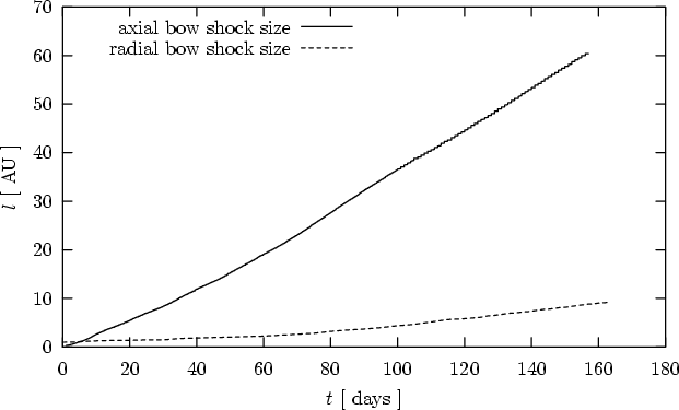	Figure 4: Size of the bow-shock in axial and radial direction for model i$^\prime$. After a phase of constant radial extent and therefore acceleration of the axial bow-shock, the jet head grows, leading to a constant propagation velocity of the jet.
Open with DEXTER

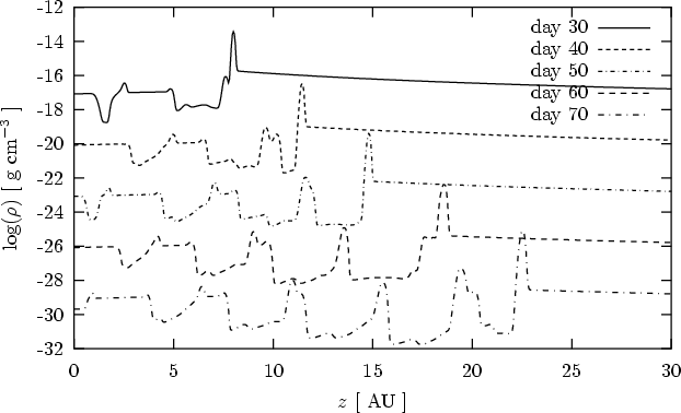Figure 5: Slices of density along the jet axis for model i$^\prime$ at days 30, 40, 50, 60, and 70, respectively. The last four lines are shifted downwards by 3, 6, 9, and 12 orders of magnitude, respectively, for clarity. After day 70, the density of the first internal shock behind the bow-shock is larger than the density of the surrounding medium, which then leads to the substantial change in kinematics.

Open with DEXTER

After day 70, the density of the first internal shock behind the bow-shock is larger than the local density of the surrounding medium. As this first internal shock hits the bow-shock region and therefore continues to drive the propagation of the entire jet, this balance, i.e. the transition from an initially underdense to an overdense jet, leads to the substantial change in kinematics described above. The same scenario also holds for model iv, the velocity of the jet head is about 700 km s^-1.

4.2 Internal jet structure

As in the old model i with cooling, the propagation of all pulses again can be traced until their merger with the jet head. Each new pulse is instantaneously slowed down from 2000 km s^-1 to about 1200 km s^-1 within the first two days. The distance between the internal shocks created by the periodic velocity pulses stays constant. The very simple, periodic jet structure in the axial cuts of the Mach number, axial velocity, density, pressure, and temperature - showing knots and the jet beam - remains unaffected in this large scale simulation by the aforementioned transition.

A difference between model i$^\prime$ and the former model i with cooling is the radial extent of these knots (Fig. 6). The whole width of the jet, however, is again taken by the jet beam, i.e. by unshocked jet material. A cocoon of shocked jet matter is only a very small shell close to the contact discontinuity, and a backflow is again absent. Therefore the basic composition of the jet is not changed, only the dimensions. While in model i with cooling, the knots had a radius of 1 AU, their extent is now a few AU. The density level in the knots, however, is lowered by a factor of ten. Therefore the total mass of each knot could be constant during this spreading process, which could be triggered by a trough in the pressure profile at an intermediate jet length. There also, the temperature and the sound speed are reduced, leading to large Mach numbers.

The axial velocity component stays nearly constant inside the jet, but is slightly enhanced at radii of 5 AU compared to the jet axis. This leads to a slow overtaking of the radial extensions of the jet pulses. The radial velocity component shows negative velocities, i.e. towards the axis, at larger distances near the jet axis. This seems to be another result of this overtaking, leading to an eddy-like structure near the jet head.

Another feature in the radial velocity is the linear, Hubble-like increase at lower distances from the jet axis. This is often seen in Planetary Nebulae (e.g. Corradi et al. 2001) and can be explained by a fast wind traveling into a self-similar 1/r² density profile (e.g. Koo & McKee 1992). As the radial velocities are still of the order of a few hundred km s^-1, a radial radiative dense shell of shocked ambient medium is present.

	Figure 6: Logarithm of density for model i$^\prime$ on day 162 and for model iv$^\prime$ on day 115. The extent of the knots in the jet beam is enlarged with respect to the former model i with cooling. No cocoon and no backflow are present; in model iv$^\prime$ the internal structure is more complicated than in model i$^\prime$ and the knots are drifting away from the jet axis.
Open with DEXTER

Figure 7: Radiative properties of model i$^\prime$ on day 162 ( left) and model iv$^\prime$ on day 115 ( right): the emissivity of bremsstrahlung and optical emission in erg s-1 cm-3, emission maps of bremsstrahlung and optical emission in erg s-1 cm-2 with an assumed distance of 200 pc - with and without a detection threshold of 10-15 erg s-1 cm-2. The emission of the internal knots is blended by the emission of the dense radiative shell of shocked ambient medium.

Open with DEXTER

In model iv$^\prime$, the internal knots are also extended in radial size, but are no longer pronounced as in model i$^\prime$ along the full width of the jet. Instead of the clear crescent form in model i$^\prime$, the structure of the knots is now more complicated. Furthermore, they are drifting away from the jet axis while traveling and do not hit the jet head, but the lateral shock, leading to a sharp step. Therefore the pulses are not able to transfer the full momentum to the propagation of the jet head.

   
5 Radiative properties of the jets

   
5.1 Emission maps

Using the density and pressure data in each grid cell of model i$^\prime$, we can calculate the temperature, the ionization fraction $X = n_{\rm e} / n_{\rm H}$, and then the total emissivity due to bremsstrahlung using the formula

$$j = 1.68 \times 10^{-27}~T^{1/2}~n_{\rm e}~n_{\rm i}~ \rm {erg~s}^{-1} \rm {cm}^{-3}$$ (3)

according to e.g. Rybicki & Lightman (1979). We also calculate the optical emissivity of Balmer lines (Aller 1984) using

$$j = 4.16 \times 10^{-25} ~ T_{4}^{-0.983} ~10^{-0.0424/T_{4}}~n_{\rm e}~n_{\rm i}~ \rm {erg~s}^{-1} \rm {cm}^{-3}$$ (4)

with T₄ the temperature in units of 10⁴ K. Both emissivities are plotted in the first two rows of Fig. 7.

These emissivities are then rotated and integrated along a line of sight that is perpendicular to the jet axis. Assuming a distance of 200 pc to the observer, emission maps are created (Fig. 7, rows 3 and 5). The emission above a detection threshold of 10^-15 erg s^-1 cm^-2 is also given.

In the emissivity plots, the knots with high density and lower temperature can be well detected because of their emission which is higher than that of the jet beam with its low density and higher temperature. The distinctness of these structures in the cocoon increases downstream towards the jet head and allows them to be detected more easily. After creating emission maps, however, the emission of the knots is blended by a strong emission of the dense radiative shell of shocked ambient medium.

The parts above the threshold show several distinct features that are created not by the knots, but by emission variations in this shell. As axisymmetry was assumed, these features are rings around the jet, observed as stripes at high inclinations.

   
5.2 The absorption line profiles

In Paper I, the calculations of the jet absorption profiles have been presented in detail. Again, we start with a normalized continuum emission and a Gaussian emission line profile:

$$I_{0} = 1 + I_{\rm peak} \cdot \exp{\left( - v^2/\sigma^2 \right)} .$$ (5)

The initial continuum and line emission (5) are taken as input for the innermost grid cell of each path. We then calculate the absorption within each grid cell j along the line of sight according to:

 

$$I_{j-1} \cdot {\rm e}^{-\tau_\lambda}$$                            I_j =

$$\tau_\lambda \frac{\pi ~ e^2}{m_{\rm e} ~ c} ~ \lambda_{kl} ~ \left( 1 - \frac{v_{j}}{c} \right) ~ \frac{\rho_{j}~\eta}{m_{\rm H}} ~ \Delta x_{j}~f_{kl}$$ =

$$\mathcal{C}_{kl}~\Delta x_{j}~\mathcal{F}(v_{j},\rho_{j})~,$$ = (6)

where e is the electron charge, $m_{\rm e}$ the electron mass, c the speed of light, $\lambda_{kl}$ the rest frame wavelength of the transition, $m_{\rm H}$ the proton mass, and f_kl the oscillator strength. The parameters are constant for a given atomic transition. We choose the Ca II K transition here with $\lambda_{kl}=3934$ Å. $\Delta x_{j}$ is the length of the path through grid cell j, which is a function of the inclination i.

The parameters depending on the different hydrodynamical models are the velocity projected onto the line of sight v_j, the mass density $\rho_{j}$, and $\eta$ the relative number density with respect to hydrogen $\eta=n_k/n_{\rm H}$ of the absorbing atom in the lower level k of the investigated line transition. The velocity is binned for the calculation of the absorption. The size of the bins $\Delta v$ can be interpreted as a measure of the kinetic motion and turbulence in one grid cell. This absorption dispersion helps to smooth the effects of the limited spatial resolution of the numerical models. The absorption calculation through the jet region is then repeated for all possible light paths from the emission region to the observer. The arithmetic mean of the individual absorption line profiles from each path is then taken as the resulting spectrum.

In Paper I, we described that the high-velocity components in the synthetic absorption line profiles are not as pronounced as in the observed ones. Now, our model iv$^\prime$ could be a solution to that problem, since both ways of increasing the absorption in the high velocity components - higher pulse density and the cooling treatment - are now present. The parameters are now chosen as in the best-fit model in Paper I: $I_{\rm peak}=6$, $\sigma=100$ km s^-1, $\lambda_{kl}=3934$ Å, f_kl=0.69, $\eta=2 \times 10^{-6}$ for the Ca II K transition, $\Delta v =10$ km s^-1, $i=0^\circ$, and $r_{\rm em}=1$ AU.

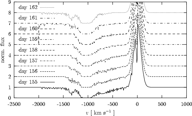	Figure 8: Sequence of absorption line profiles for eight consecutive days for model i$^\prime$.
Open with DEXTER

	Figure 9: Sequence of absorption line profiles for eight consecutive days of model iv$^\prime$.
Open with DEXTER

In Figs. 8, 9, the sequences of eight consecutive nights of the two large-scale models i$^\prime$ and iv$^\prime$ are shown. In the first case, the extension of model i$^\prime$ to longer propagation times and larger lengths create only slight differences compared to Fig. 26 (bottom) in Paper I. The position of the main absorption trough, the shape of its boundaries, the presence, persistence, and depth of the high velocity component are all very similar to those in the former model i with cooling. The absorption in the center of the emission line is created by the ambient medium in front of the jet.

The model iv$^\prime$ with increased jet pulse densities, however, creates clearly visible differences. The stable absorption trough is shifted towards higher velocities, from -1050 km s^-1 up to -1300 km s^-1, and its width is increased from about 200 km s^-1 to 500 km s^-1. In the high velocity component, several deep absorptions are present in contrast to the few moderate ones in model i$^\prime$.

6 Summary and discussion

In this paper, we present results of two new hydrodynamical simulations, including radiative cooling. They were started due to a drawback in our former simulations presented in Paper I (Stute et al. 2005), which were stopped close to density balance of the jet and the ambient medium. As underdense and overdense jets behave in different ways and as the kinematics of the jets was a main result in Paper I, we expected new insights.

Another point is that a few minor differences between the models and the observations were thought to be solved by a model with an increased jet density during the pulses - model iv$^\prime$ - which was calculated only with purely hydrodynamical means in the former grid of simulations. Therefore, we performed two hydrodynamical simulations with an approximated cooling treatment beyond this density balance, one with the same parameters as model i in Paper I, which was presented there with and without cooling, and the second with higher gas densities in the jet pulses, as in model iv.

Since in the new cooling treatment ionization fractions of collisional ionization equilibrium (CIE) were used and not self-consistent general non-equilibrium (NEQ) rate equations, we discussed the possible effects of underestimating the ionization fraction of hydrogen and validated this cooling treatment by comparing density and temperature values of the gas parcels in the jet, as well as by showing plots of the ionization fraction itself. We saw that the differences are only very small.

In Paper I, the jet in model i with cooling had a constant cross section over the simulated 74 days. This led to an accelerated motion with high velocities of 730 km s^-1, while the velocity of the adiabatic jet was only about 200 km s^-1. The extended model i$^\prime$ in this paper now shows that after the first 70 days the transition from an underdense to an overdense jet lets the cross section inflate and therefore compensate for the density profile of the external medium. The acceleration is stopped and the jet then has a constant velocity of about 740 km s^-1. Thus, the transition results in a completely different motion. The conclusion that the high observed velocities in CH Cygni, R Aquarii, and MWC 560 favor the models with cooling is unchanged by the transition.

The radial inflation mentioned above also changes the internal structure of the jet. The width of the internal knots is also increased, as the basic composition of the jets is not affected. The cocoon of shocked jet matter is again confined to a small shell close to the contact discontinuity and the whole jet lobe is filled with unshocked jet material. In model i$^\prime$, these knots are very pronounced along their width, while their structure is not intact in model iv$^\prime$.

These knots are the locations of enhanced bremsstrahlung and optical emissivity, which is therefore again more pronounced in model i$^\prime$. These knots could be identified with the observed parallel features in R Aquarii (Paresce & Hack 1994). After rotating the emissivity plots and integrating them, however, other features become more prominent. The internal knots are blended by the emission of the dense radiative shell of shocked ambient medium. As they are spatially variable, parallel rings of enhanced emission are created by the rotation and also look similar to the observations, if one keeps in mind that axisymmetry was assumed in our model. Without that, the shapes of the features on the shell should be different.

The observed length of the jet in R Aquarii is several hundred AU, thus much larger than in our simulations. At larger distances from the source, however, the density of the ambient medium drops by another order of magnitude, making it likely that the relative contribution of the emission of the knots will increase.

Concerning the absorption line profiles, no large differences between the former model i with cooling and the recent model i$^\prime$ are visible. This means that the influence of the age of the jet on the profiles should only be marginal. In model iv$^\prime$, however, differences arise. The stable absorption trough is shifted toward higher velocities, from -1050 km s^-1 up to -1300 km s^-1, and its width is increased from about 200 km s^-1 to 500 km s^-1. In the high velocity component, several deep absorptions are present in contrast to the few moderate ones in model i$^\prime$.

Both results highly increase the ability of the model to reproduce the observed absorption line profiles (see Fig. 1 in Paper I or Schmid et al. 2001). We can say here that the real parameters in MWC 560 are closer to model iv$^\prime$ than to model i$^\prime$.

As the pulse structure was not changed, the line widths of the high velocity components are again quite narrow. This could perhaps be improved by using a sinusoidal or Gaussian pulse profile, instead of the rectangular steps in velocity and density, and also a spatial velocity and density profile, instead of the constant values within the jet nozzle.

Acknowledgements

The author wants to thank the High Performance Computing Center Stuttgart for allowing him to perform the expensive computations, and H. M. Schmid and M. Camenzind for fruitful discussions. We acknowledge the constructive comments and suggestions by the referee.

References

• Aller, L. H. 1984, Physics of Thermal Gaseous Nebulae (Dordrecht: D. Reidel Publishing Company) (In the text)
• Corradi, R. L. M., Livio, M., Balick, B., Munari, U., & Schwarz, H. E. 2001, ApJ, 553, 211 [NASA ADS] [CrossRef] (In the text)
• de Gouveia dal Pino, E. M., & Cerqueira, A. H. 2002, RMxAA, 13, 29
• Eyres, S. P. S., Bode, M. F., Skopal, A., et al. 2002, MNRAS, 335, 526 [NASA ADS] [CrossRef] (In the text)
• Hollis, J. M., Michalitsianos, A. G., Kafatos, M., et al. 1985, ApJ, 289, 765 [NASA ADS] [CrossRef]
• Hollis, J. M., Lyon, R. G., Dorband, J. E., et al. 1985, ApJ, 475, 231 [NASA ADS] [CrossRef]
• Kellogg, E., Pedelty, J. A., & Lyon, R. G. 2001, ApJ, 563, 151 [NASA ADS] [CrossRef]
• Koo, B.-C., & McKee, C. F. 1992, ApJ, 388, 103 [NASA ADS] [CrossRef] (In the text)
• Paresce, F., & Hack, W. 1994, A&A, 287, 154 [NASA ADS]
• Rybicki, G. B., & Lightman, A. P. 1979, Radiative Processes in Astrophysics (New York: John Wiley & Sons) (In the text)
• Schmid, H. M., Kaufer, A., Camenzind, M., et al. 2001, A&A, 377, 206 [EDP Sciences] [NASA ADS] [CrossRef] (In the text)
• Solf, J., & Ulrich, H. 1985, A&A, 148, 274 [NASA ADS]
• Steffen, W., Gomez, J. L., Williams, R. J. R., et al. 1997, MNRAS, 286, 1032 [NASA ADS]
• Stone, J. N., & Norman, M. L. 1993, ApJ, 413, 198 [NASA ADS] [CrossRef]
• Stute, M., Camenzind, M., & Schmid, H. M. 2005, A&A, 429, 209 [EDP Sciences] [NASA ADS] [CrossRef] (Paper I) (In the text)
• Sutherland, R. S., & Dopita, M. A. 1993, ApJS, 88, 253 [NASA ADS] [CrossRef] (In the text)
• Taylor, A. R., Seaquist, E. R., & Mattei, J. A. 1986, Nature, 319, 38 [NASA ADS] [CrossRef] (In the text)
• Thiele, M. 2000, Numerical simulations of protostellar jets, Ph.D. Thesis, University of Heidelberg (In the text)
• Ziegler, U., & Yorke, H. 1997, Comp. Phys. Comm., 101, 54 [NASA ADS] (In the text)