A&A 450, 509-521 (2006)
DOI: 10.1051/0004-6361:20053590
Low and intermediate mass star yields
II. The evolution of nitrogen abundances
M. Gavilán1 -
M. Mollá2 - J. F. Buell3
1 - Departamento de Física Teórica, Universidad Autónoma
de Madrid, 28049 Cantoblanco, Spain
2 - Departamento de Investigación Básica,
C.I.E.M.A.T., Avda. Complutense 22, 28040 Madrid, Spain
3 - Department of Mathematics and Physics, Alfred State College,
Alfred, NY 14802, USA
Received 7 June 2005 / Accepted 25 November 2005
Abstract
Aims. We analyze the impact on the Galactic nitrogen abundances with a new set of low and intermediate mass star yields. These yields contain a significant yield of primary nitrogen from intermediate mass stars.
Methods. We use these yields as an input for a galactic chemical evolution model and study the nitrogen abundances in the halo and in the disc, and compare them with models obtained using other yield sets and with a large amount of observational data.
Results. We find that with these new yields our model reproduces the observed trends adequately. In particular, these yields solve the historical problem of nitrogen evolution, giving the right level of relative abundance N/O by producing a primary component in intermediate mass stars. Moreover, using different evolutionary rates for each radial region of the Galaxy, we can explain the observed N dispersion.
Key words: galaxies: abundances - galaxies: evolution -
galaxies: spirals
Most elements are created in the interiors of stars by nucleosynthesis
processes (see Wallerstein et al. 1997, for a review), starting with hydrogen
and progressing toward heavy elements. These processes are called primary production. Some elements, however, can be formed from
heavier nuclei than the hydrogen originally present in the star. They
are called secondary. This is the case for nitrogen, which can
be created during the CNO cycle using seeds of original carbon and/or
oxygen. From a theoretical point of view, it has been considered that
massive stars produce secondary nitrogen (Peimbert 1987), while low and
intermediate mass (LIM) stars have mechanisms, like the third
dredge-up and the hot bottom burning (HBB) processes, to produce both
primary and secondary nitrogen (Alloin et al. 1979; Edmunds & Pagel 1978). The third
dredge-up event is a consequence of the thermal pulses in the star,
and transport C and He to the outer layers. The HBB occurs when the
CNO cycle takes place at the base of the convective envelope.
Observationally, there are several open questions about the primary or
secondary character of nitrogen that up to now remain unsolved. When N
and O data are represented as log(N/O) vs. log(O/H), including
the galactic stars, H II regions for the Milky Way Galaxy (MWG),
external galaxies (Garnett et al. 1995; Izotov & Thuan 1999; van Zee et al. 1998a; Garnett et al. 1999), and the high
redshift data (Pettini et al. 2002; Prochaska et al. 2002; Centurión et al. 2003, and references therein), a
clear positive slope appears for abundances larger than
 dex, which indicates a secondary behavior; but the
plot shows a flat slope for low metallicities that can only be
explained with a primary component of nitrogen. Taking into account
that this flat slope occurs for low abundances, the first idea
proposed, shared by some authors (Diaz & Tosi 1986; Pagel et al. 1979; Dahmen et al. 1995) is that
observations would be reproduced if the nitrogen ejected by massive
stars were primary, while intermediate mass stars might have both
primary and secondary components.
dex, which indicates a secondary behavior; but the
plot shows a flat slope for low metallicities that can only be
explained with a primary component of nitrogen. Taking into account
that this flat slope occurs for low abundances, the first idea
proposed, shared by some authors (Diaz & Tosi 1986; Pagel et al. 1979; Dahmen et al. 1995) is that
observations would be reproduced if the nitrogen ejected by massive
stars were primary, while intermediate mass stars might have both
primary and secondary components.
Thus, some authors have tried to look for mechanisms that explain how
massive stars could produce primary nitrogen. This is the case of
Meynet & Maeder (2002) who have recently proposed rotation as a possible source
of primary nitrogen, since low metallicity stars show a bigger
rotation than high metallicity ones. Chiappini et al. (2003a) used these yields
in their chemical evolution models, concluding that they are only a
lower limit for the primary nitrogen production since the HBB is not
considered in their calculation. In fact, Chiappini et al. (2005) find that an
extra production of N in low metallicity massive stars by a large
factor, between 40 and 200 along the mass range, is necessary to
explain the data of very metal-poor halo stars since these yields do
not produce a sufficient amount of primary N. Moreover, if the
production of primary nitrogen proceeded from massive stars, the left
side of the (N/O) vs. (O/H) plot should not show any scatter.
Although some authors claim to observe (Pilyugin et al. 2003; Izotov & Thuan 1999) this lack
of scatter, recent observations from low metallicity objects
(Israelian et al. 2004; Spite et al. 2005; Pettini et al. 2002; Prochaska et al. 2002; Centurión et al. 2003) do show a clear dispersion.
Serrano & Peimbert (1983) have already claimed that a secondary production by
intermediate mass stars must exist and suggested that the zero slope
may be explained by two factors: 1) a delay in the ejection of N to
the ISM due to the different mean-lifetimes of stars and 2) the gas
infall effects. The advantage of taking a delay into account is that
the large data scatter can be explained by considering different
evolutionary states for each galaxy, so this possibility has been
supported by a large number of authors:
Pilyugin (1992); van Zee et al. (1998b); Pilyugin (1993); Henry et al. (2000); Vila Costas & Edmunds (1993). This last group also includes
gas flows - infall or/and outflow - and low efficiency for the star
formation rate (the equivalent mechanism to produce a delay) in the
low evolved regions, in order to reproduce the flat slope in the (N/O) vs. (O/H) plot. They conclude that the secondary production of
nitrogen should dominate in high metallicity environments, while the
primary one should act at low metallicities.
Some new yields for LIM stars were given in Gavilán et al. (2005, hereinafter Paper
I), where they were adequately evaluated and calibrated by
using them in a Galaxy chemical evolution model. It was shown that the
results about C and O abundances reproduce the Galactic and Solar
Neighborhood data adequately. The purpose of this work is to analyze
the impact of these stellar yields on the nitrogen abundances. In
particular, we use the same prescriptions of Paper I to check if the
contribution to N given by these yields for LIM stars is sufficient to
justify the amount of primary nitrogen the observations point to.
We describe the yields in Sect. 2, analyzing in particular the primary
and secondary components of the nitrogen production. In Sect. 3 we
briefly describe the chemical evolution model. Section 4 is devoted to
the results, and the conclusions are presented in Sect. 5.
2 Low and intermediate mass yields:
the secondary and primary components of nitrogen
The aim of this work is the study of the nitrogen behavior, using the
same set of yields as in Paper I, that we call BU yields. For
comparison purposes we also take the LIM stars yields from
van den Hoek & Groenewegen (1997) and Marigo (2001) that we call VG and MA, respectively.
The complete table of BU yields was already given in Paper I for five
metallicities: -0.2, -0.1, 0.0, +0.1, and +0.2, expressed as
 ,
where solar abundances were taken from Grevesse & Sauval (1998)
,
where solar abundances were taken from Grevesse & Sauval (1998)![[*]](/icons/foot_motif.gif) .
.
![\begin{figure}
\par\includegraphics[width=7.8cm,clip]{3590f1.eps}
\end{figure}](/articles/aa/full/2006/17/aa3590-05/Timg12.gif) |
Figure 1:
Total yields (BU) of: a) 12C and b) 14N
produced by LIM stars for different metallicities following label
on panel b), expressed as
.
|
| Open with DEXTER |
We summarize the behavior of the carbon and nitrogen yields for LIM stars, as shown in Fig. 1. In panel a) we see that the
12C yield is extremely small for stars with mass lower than 2  ,
since they do not experience third dredge up events.
However, stars begin to suffer these kinds of events for smaller
masses at lower metallicity. In other words, in the low mass range,
the metallicity and the 12C yield are anti-correlated. When the
stars have enough mass to undergo HBB, the 12C yield drops
abruptly because of the conversion of carbon into nitrogen. The
14N yield presents a local maximum in the mass range from 3.5 to 5 ,
depending on the metallicity, then decreases before
beginning to increase again as a function of stellar mass. The
largest amount of nitrogen is produced by stars of intermediate mass
because HBB and the 2nd dredge-up occur only in stars with
,
since they do not experience third dredge up events.
However, stars begin to suffer these kinds of events for smaller
masses at lower metallicity. In other words, in the low mass range,
the metallicity and the 12C yield are anti-correlated. When the
stars have enough mass to undergo HBB, the 12C yield drops
abruptly because of the conversion of carbon into nitrogen. The
14N yield presents a local maximum in the mass range from 3.5 to 5 ,
depending on the metallicity, then decreases before
beginning to increase again as a function of stellar mass. The
largest amount of nitrogen is produced by stars of intermediate mass
because HBB and the 2nd dredge-up occur only in stars with
 .
As the HBB increases the luminosity and the
mass-loss rate, stars that suffer this process have shorter TP-AGB
lifetimes. The local maximum occurs in the transition between stars
with HBB and those without. The increase at higher masses is due to
the shortened time between third dredge-up events. The yields at the
lowest masses are due to the 1st dredge-up.
.
As the HBB increases the luminosity and the
mass-loss rate, stars that suffer this process have shorter TP-AGB
lifetimes. The local maximum occurs in the transition between stars
with HBB and those without. The increase at higher masses is due to
the shortened time between third dredge-up events. The yields at the
lowest masses are due to the 1st dredge-up.
![\begin{figure}
\par\includegraphics[angle=-90,width=11.4cm,clip]{3590f2.eps}
\end{figure}](/articles/aa/full/2006/17/aa3590-05/Timg15.gif) |
Figure 2:
The ratio of the yield of primary
 to the total
yield of
as derived from different author sets: BU, VG,
and MA. Panel a) a comparison of the solar metallicity yields for the
three sets as labeled. Models for two different compositions, as
labeled, are represented in panels b), c), and d) for BU, MA, and VG,
respectively.
to the total
yield of
as derived from different author sets: BU, VG,
and MA. Panel a) a comparison of the solar metallicity yields for the
three sets as labeled. Models for two different compositions, as
labeled, are represented in panels b), c), and d) for BU, MA, and VG,
respectively. |
| Open with DEXTER |
The most important difference among the used yields resides in the
contribution of primary and secondary components of nitrogen by LIM stars. In Fig. 2 we represent the fraction of primary 14N for the three sets used, as labeled, as a function of mass (
 ,
except for MA, for which
,
except for MA, for which
 ). In panel a) we show the results for solar abundances.
All of them show a similar behavior with a maximum for masses around 3.5-4 .
). In panel a) we show the results for solar abundances.
All of them show a similar behavior with a maximum for masses around 3.5-4 .
We must clear up some points about the components of N. The only
difference between primary and secondary nitrogen is the origin of the
carbon atom producing it. Although the idea is conceptually clear, it
is not so simple to separately compute both components. Thus, although
BU and MA give the two components separately for each model, VG do
not. These authors, however, show their yields in each phase of
stellar evolution. If we consider that all the nitrogen created in
the AGB phase is primary, about  90% of the N ejected by LIM stars will be primary. This is sometimes assumed when these yields are
used. This hypothesis, which we call AGB technique leads to a
primary N component that is excessively large and is not totally
adequate.
90% of the N ejected by LIM stars will be primary. This is sometimes assumed when these yields are
used. This hypothesis, which we call AGB technique leads to a
primary N component that is excessively large and is not totally
adequate.
Let us return to the definition: secondary N proceeds from the burning
of original 12C. If a fraction of the original carbon is burned
in the pre-AGB phase, it produces secondary N. Sometimes, this gives
a negative 12C yield. But, not all the initial carbon is consumed
before the AGB phase. If we take a star of 4
of solar
abundance as an example, that is, with
 ,
it has an initial 12C mass
,
it has an initial 12C mass
 .
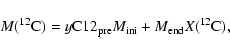
The pre-AGB phase carbon yield is
.
The pre-AGB phase carbon yield is
 ,
so the mass of this element present in the star
before the AGB begins is:
,
so the mass of this element present in the star
before the AGB begins is:
 |
(1) |
where
 is the mass of the star at the end of this first
phase: 3.95
is the mass of the star at the end of this first
phase: 3.95
 .
Therefore, there is a mass
.
Therefore, there is a mass
 of 12C, from which
 corresponds to the original carbon. This
implies that a quantity of the original carbon is still available to
form nitrogen in the following phases. Thus, a fraction of the total
nitrogen produced in the AGB phase (given by the addition of the two
values given by VG in their tables denoted AGB yields and final AGB yields) may be secondary. In order to calculate this component from
the total AGB yields, we use the fraction, called r, between the
secondary to the total nitrogen yield,
corresponds to the original carbon. This
implies that a quantity of the original carbon is still available to
form nitrogen in the following phases. Thus, a fraction of the total
nitrogen produced in the AGB phase (given by the addition of the two
values given by VG in their tables denoted AGB yields and final AGB yields) may be secondary. In order to calculate this component from
the total AGB yields, we use the fraction, called r, between the
secondary to the total nitrogen yield,
 N. Taking
into account that the secondary N proceeds from the existing carbon
used as a seed, we assume that r is equal to the ratio between the
old carbon and the new-plus-old carbon:
N. Taking
into account that the secondary N proceeds from the existing carbon
used as a seed, we assume that r is equal to the ratio between the
old carbon and the new-plus-old carbon:
 |
(2) |
This method (hereinafter called r method), may be applied only to
stars that suffer the HBB and produce primary 14N, that is, those
for which the core mass before the HBB is larger than
 ,
usually stars with
,
usually stars with
 .
Otherwise, the
nitrogen yield is totally secondary. The results of VG shown in
Fig. 2 proceed from this calculation.
.
Otherwise, the
nitrogen yield is totally secondary. The results of VG shown in
Fig. 2 proceed from this calculation.
We have then computed the integrated yields of 14N produced by
LIM stars that we present in Fig. 3 as a
function of metallicity Z. In panel a), we represent the BU results
as solid circles on which we have performed a least-squares fit shown
by the solid (red) line. This integrated yield for 14N,
equivalent to the yield produced by a single stellar population, is
located between the two other sets in this panel, showing a similar
dependence on Z as VG but with lower absolute values.
More significant, however, is how the ratio of primary
to total integrated yields,
 N depends on metallicity,
shown in panel b). This ratio increases for decreasing metallicity for all
sets, as expected, although the integrated yield for VG is quite
different if we consider the AGB technique rather than the r method.
N depends on metallicity,
shown in panel b). This ratio increases for decreasing metallicity for all
sets, as expected, although the integrated yield for VG is quite
different if we consider the AGB technique rather than the r method.
This metallicity effect can be easily explained: low metallicity stars
have smaller radii and take longer to reach super-winds, so they have
more time to experience third dredge-up events than solar metallicity
stars. As a consequence, they have more fresh
 in their
envelopes and can make more primary nitrogen by the HBB process. On
the other hand, due to the lower amount of original carbon, they
produce, obviously, less secondary nitrogen. For VG yields the ratio
is almost constant at a value of 15% with the r technique,
represented by the short-dashed (blue) line, for metallicities greater
then 0.01, increasing for metallicities lower than this value. While
it is 90% when the AGB technique, represented by a
dot-short-dashed (blue) line, is used, showing a smooth variation with Z. It is interesting that the integrated yield for solar abundance in
the BU case is around 20%,
very similar to the value computed as necessary by Alloin et al. (1979) two
decades ago on the basis of the observations available at that time.
in their
envelopes and can make more primary nitrogen by the HBB process. On
the other hand, due to the lower amount of original carbon, they
produce, obviously, less secondary nitrogen. For VG yields the ratio
is almost constant at a value of 15% with the r technique,
represented by the short-dashed (blue) line, for metallicities greater
then 0.01, increasing for metallicities lower than this value. While
it is 90% when the AGB technique, represented by a
dot-short-dashed (blue) line, is used, showing a smooth variation with Z. It is interesting that the integrated yield for solar abundance in
the BU case is around 20%,
very similar to the value computed as necessary by Alloin et al. (1979) two
decades ago on the basis of the observations available at that time.
![\begin{figure}
\par\includegraphics[width=7.8cm,clip]{3590f3.eps}
\end{figure}](/articles/aa/full/2006/17/aa3590-05/Timg33.gif) |
Figure 3:
a) Dependence of the integrated yield of 14N produced by
LIM stars on metallicity for the three yield sets, marked with
different symbols as in Fig. 2. The crosses are the
results obtained by Henry et al. (2000) for the same VG yields using a
Salpeter IMF. b) The ratio between the primary to the total nitrogen
yield with the same symbols than in panel a). The two possible
techniques to compute the primary component of VG yields are
represented as short-dashed line (method r) and dot-short-dashed
line (method AGB). |
| Open with DEXTER |
All these considerations indicate that the primary nitrogen appears on
a different time scale in the ISM depending on the value of Z. The first
primary N will be ejected when stars of 8
die (5 for MA),
while Z is still low.
The model used in this work is the multiphase chemical evolution model
described in Ferrini et al. (1994,1992), in the version presented in
Mollá & Díaz (2005), and in Paper I. For LIM stars, we used the same yields BU as in these two last papers, and for comparison purposes, those
from MA and VG. For massive stars we chose Portinari et al. (1998) and
Woosley & Weaver (1995, hereinafter PCB and WW, respectively). We ran
different models computed with different combination of yields: BU +
WW, VG + WW, and MA + PCB, which we distinguish as BU, VG, and MA,
respectively.
The nitrogen study is usually done by comparing its behavior relative
to iron and oxygen, so it is very important to have a careful
calibration for these two elements. Oxygen calibration was done in
Paper I. The SNIa are the main manufacturer of iron. The yields for
type Ia supernova (SNIa) explosions are taken from Iwamoto et al. (1999) and
Branch & Nomoto (1986). The evolution of this element in the model is
quasi-independent of the normal stars yields. However, since iron is
mainly produced by SNIa, even if its yield is very well known, its
abundance is very dependent on the method of computing the rate of
these explosions. For this purpose we analyzed the results obtained
with different possibilities in order to eliminate, if possible,
uncertainties in the iron abundance evolution. This point is
relatively important because the Age-metallicity relation and the
G-dwarf metallicity distribution are usually used as calibration
methods for chemical evolutions models. Furthermore, we go on to
compare our results with observed stellar nitrogen abundances, most of
which are given as [N/Fe], so, we checked that the Iron evolution is
adequately reproduced by our models before this comparison be made.
We used three methods to compute the SNIa rates as given by the
following authors: the classical one (Matteucci & Greggio 1986; Ferrini & Poggianti 1993), the one
given by Tornambe (1989), and the last, more recent, described in
Ruiz-Lapuente et al. (2000), hereinafter MAT, TOR, and RL, respectively. The first
authors estimate the SN rates by using only the initial mass
function. We summarize her the method that is well explained in the first
two cited works: a proportion of the stellar masses in a given
range [
 ]
will be in binary systems and a fraction
of them will develop type Ia supernova. Based on this idea, a mass
function for the secondary stars is computed from the original
one. Finally the SNIa rate depends on the number of secondary stars
that died in each time step, which implies that the time scale for the
iron appearing in the ISM is controlled by the mean lifetimes of these
secondary stars.
]
will be in binary systems and a fraction
of them will develop type Ia supernova. Based on this idea, a mass
function for the secondary stars is computed from the original
one. Finally the SNIa rate depends on the number of secondary stars
that died in each time step, which implies that the time scale for the
iron appearing in the ISM is controlled by the mean lifetimes of these
secondary stars.
Actually, this time scale does not depend only on the secondary mean
lifetimes, since there are other processes that also participate in
the conversion of a binary system into a SNIa explosion. It is
necessary to take into account the effects of the distances between
both stellar components, the orbital velocities, and other parameters
to finally obtain the time taken for the system to explode after the
moment of its formation. Tornambe (1989) performed these calculations
for several combinations of possible candidates of binary system or
SNIa scenarios (double degenerate, single degenerate, etc.), thereby
providing the supernova rate as a function of time normalized for a
binary system of 1 .
All the physical processes and
assumptions are included in their calculations, so we only need to
include the selected functions in our code and multiply them by the
number of binary systems, avoiding the need to compute the secondary
and primary initial mass functions necessary in the first method.
A similar technique was also performed more recently
by Ruiz-Lapuente et al. (2000) who provides us with a numerical table (private
communication) with the time evolution of the supernova rates for a
single stellar population, computed under updated assumptions about
different scenarios and probabilities of occurrence. We computed the
supernova rates using the three methods, thus producing three models
MAT, TOR, and RL. These different techniques mostly affect the iron
abundances, the other elemental abundances being equal for all of
them. Therefore, we will compare the three types of SN rate
calculations by using only BU yields in the analysis of the iron
abundance evolution, as well as in the calibration of the model (next
section). We will compare the three set of LIM stars yields when N is
studied, using only the RL technique. Only for the comparison of the
relative abundance [N/Fe] we will show the nine possible combinations
of models.
![\begin{figure}
\par\includegraphics[width=11.4cm,clip]{3590f5.eps}
\end{figure}](/articles/aa/full/2006/17/aa3590-05/Timg36.gif) |
Figure 5:
Age-metallicity relation: a) for the BU and RL model dividing
WW iron yield by 1, 1.5, 2, and 2.5. b) using MAT, TOR, and RL SNIa
rates with BU yields dividing the WW iron yield by 2. Data are from authors
of Table 1 as labeled. |
| Open with DEXTER |
The main disparity among the three techniques described above resides
in the different evolutions of the SN rate in time. As we see in
Fig. 4, MAT is the technique that presents highest values of
SNIa/SNII at any time, reaching the maximum at 2.5 Gyr. RL has a
maximum between 2 and 5 Gyr, with values approximately 1/2 or 1/3 of
those given by MAT. The TOR model is the only one with low values.
Even if it presents a maximum before the first Gyr, this will not be
seen in the results because its value is very small. From the first Gyr, SNIa/SNII has positive slope and almost reaches the observed
value at the present time. Nevertheless, all of them still are within
the error bar given by observations (Cappellaro et al. 1999; Cappellaro 2004; Mannucci et al. 2005). Note
that this value has been reduced for the most recent determinations
compared with the oldest ones.
The results for iron abundance obtained with these three methods are
shown in Fig. 5, the age-metallicity Relation (AMR) and in
Fig. 6, the G-Dwarf distribution, for the Solar vicinity.
For this comparison we show only BU yields, keeping in mind that the
set of yields will have only small effects on this relation.
Nevertheless, this model uses WW yields for massive stars and these
authors claim that this could produce too much iron, and advised in
Timmes et al. (1995) to divide the iron ejections at least by two. In order to
calculate how much that WW iron excess is, we calculated four
different models for BU yields and RL technique, where the iron
production of massive stars is divided by 1, 1.5, 2, and 3. Results
are represented in panel a where it is clearly shown that a factor of 2 is a good compromise that we will use in panel b. In this last panel we present the age-metallicity relation for the three SNIa
cases, where all of them are in reasonable agreement with data, given
their wide dispersion. Although there are small differences between
models, it can be seen that the iron appears later and takes a little
more time to reach high values when MAT and RL techniques are used
than for the TOR SNIa method, but all of them reach the Solar
abundance.
Regarding the G-dwarf distribution, represented in Fig. 6,
differences appear mainly between TOR and the others because it
provides a narrower distribution than the others. The three models
are able to reproduce the low metallicity tail without showing any
G-dwarf problem.
In Fig. 7 we show the relation between iron and oxygen. As
before, in panel a the BU + RL model is presented by varying the
massive stars iron ejection. In this case the differences are clearer
than in the AMR case. We chose the model Fe/2 that we use for the
rest of the paper. In panel b we plot the model results using BU yields with the three SNIa techniques. As in the previous case, the
LIM star yields do not change the results because oxygen is ejected by
massive stars and iron is mainly produced by SNIa events. In the end,
the three models have a very similar behavior.
![\begin{figure}
\par\includegraphics[width=11.5cm,clip]{3590f7.eps}
\end{figure}](/articles/aa/full/2006/17/aa3590-05/Timg38.gif) |
Figure 7:
The relation [O/Fe] vs. [Fe/H]: a) The model results for
BU + RL varying WW iron ejection; b) model BU using MAT, TOR, and RL SNIa techniques and BU yields. Open (black) dots are stellar data from
authors listed in Table 1, from which we represented the
most recent from Israelian et al. (2004) and Akerman et al. (2004) as (red) triangles and
full (blue) dots. |
| Open with DEXTER |
![\begin{figure}
\par\includegraphics[width=7.8cm,clip]{3590f8.eps}
\end{figure}](/articles/aa/full/2006/17/aa3590-05/Timg40.gif) |
Figure 8:
Time evolution of elemental abundances in the Solar vicinity
for nitrogen, as
 ;
b) nitrogen over oxygen as log(N/O);
and c) nitrogen over carbon as log(N/C). Solar abundances are the
filled symbols from Grevesse & Sauval (1998) - circle - Holweger (2001) - square -
and Asplund et al. (2005) - cross - by assuming an age of 4.5 Gyr for the sun.
Empty symbols at 13.2 Gyr are the interstellar medium abundances
given by Meyer et al. (1997,1998) - circle - and Peimbert (1999)
- square. Small open dots are stellar abundances obtained by authors
from Table 1, being those located around the Solar
vicinity (
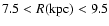
7.5 < R < 9.5 kpc). Lines meaning is given in panel a). ;
b) nitrogen over oxygen as log(N/O);
and c) nitrogen over carbon as log(N/C). Solar abundances are the
filled symbols from Grevesse & Sauval (1998) - circle - Holweger (2001) - square -
and Asplund et al. (2005) - cross - by assuming an age of 4.5 Gyr for the sun.
Empty symbols at 13.2 Gyr are the interstellar medium abundances
given by Meyer et al. (1997,1998) - circle - and Peimbert (1999)
- square. Small open dots are stellar abundances obtained by authors
from Table 1, being those located around the Solar
vicinity (
7.5 < R < 9.5 kpc). Lines meaning is given in panel a). |
| Open with DEXTER |
We devote this section to analyzing the results obtained with our
models for nitrogen abundances and comparing them with the available
observational data. We divide these results into four parts: a) the
evolution of nitrogen with time for the Solar vicinity (assumed
located at a galactocentric distance of 8 kpc), b) the radial
distributions of elements in the disc, c) the relation of log(N/O)
with the oxygen evolution, and d) the relation of [N/Fe] with iron.
Figure 8 shows the evolution of nitrogen compared with
observations in the Solar region, that is corresponding to objects at
a radial galactocentric distance between 7.5 and 9.5 kpc. Models BU,
VG, and MA are represented by the (red) solid, the (blue)
short-dashed, and the (green) long-dashed lines, respectively. Both
VG models, following the two possible techniques for calculating the
proportion of primary nitrogen, techniques r and AGB described in
Sect. 2, yield results indistinguishable for times
larger than 1 Gyr, so we represent only the results for the first one.
In panel a MA and VG models give a higher value than BU, since at the
lowest metallicity their nitrogen yield is higher than the
corresponding one from BU (see Fig. 2). Then, once an
abundance higher than 0.004 is reached, the model BU continues
increasing smoothly until the present time, reproducing both solar and
ISM abundances. The shapes shown by the three models are similar and
all of them reproduce both the solar value and the ISM value.
The same kind of information can also be extracted from the relative
abundances represented in panel b. In panel b, we show the time
evolution of log(N/O). Since there is good agreement in fitting the
abundance of oxygen for all models (see Gavilán et al. 2005), the
differences in this plot must be due only to the nitrogen
production. The disagreement between different models is important
for times shorter than 1.5 Gyr, when intermediate mass and massive
stars are the main contributors and the distinct primary/secondary
ratio effects are evident there. Model MA shows a strong increase in
the first Gyr due to the primary component, and then it
flattens. Model BU out a higher ratio of primary nitrogen than MA for
all Z except for the lowest one, which produces a smoother evolution,
and, finally, N remains below MA. The resulting final N/O ratios are
similar in both models and agree with observations. The mostly primary
behavior of the model VG, mostly when all AGB nitrogen is considered
as such, at the lowest Z, implies a very strong increase in the
abundance at the earliest times. After that, both methods give a
smooth slope, reaching an absolute value around -0.5 dex that is
higher than the observed Solar abundance.
The good behavior of BU yields is also evident in panel c where log(N/C) is shown. The MA model presents a maximum at the first Gyr,
the decrease is due to the higher amount of carbon ejected in that
model (see Paper I) so the absolute value at the present time is only
marginally reached. The shape of the VG model is similar to the BU one
but with a nitrogen excess. All models seem to fit the solar and ISM data, but the model BU is the best one for reproducing the stellar
data, and, more importantly, for fitting all of the data
simultaneously.
We now explore the radial distributions of nitrogen over the galactic
disc, as shown in Fig. 9. The data correspond to H II regions from references as labeled in the figure and to stars from
references in Table 1.
The radial distribution is reproduced more or less within the errors
by all models. Actually, the shape of the radial distribution is
fitted well in all cases, independent of the absolute values, since
this is an effect of the ratio infall/SFR along the galactocentric
radius, produced by the scenario of our MWG model, and therefore is
rather independent of the yields used. However, the observed slope of
the radial distribution at the two ends of the disc, in the center and
in the outer regions, is a matter of discussion. Thus, Vílchez & Esteban (1996)
claim that the gradients are not as steep in these regions as in the
rest of the galactic disc. The same occurs in the inner disc where the
most recent data from Smartt et al. (2001) show that the distribution
flattens. Our models have been tuned to fit these two sets of data,
causing the resulting overall gradient to be smaller than that
obtained by other authors. As can be seen in Fig. 9, MA and
VG models produce a flatter gradient than has been observed.
In Figs. 9b and 9c, the radial distributions log(N/O) and log(N/C) are plotted, as they are considered important for the study
of different yields. In panel b the radial distribution of log(N/O)
showed by data presents a clear slope, although there is some data
that shows a flatter distribution in the outer regions. A steep radial
distribution for N/O is expected because oxygen is produced by massive
stars. If nitrogen were ejected by massive stars, its secondary
character would cause it to enter the ISM after the oxygen. Instead,
if it were ejected by intermediate stars, the time needed for their
evolution would be larger. Thus, in both cases, the nitrogen appears
in the ISM after the oxygen does.
Once again, the large dispersion of the data prevents a clear
selection of the best model, however the BU model seems most
adequate for reproducing the H II region data from Vílchez & Esteban (1996)
and Fich & Silkey (1991). The MA model shows a flatter radial gradient than
the indicated by observations, with higher absolute values compared to
the mean values of data, mostly in the outer disc, and VG models, as
before, show higher values than data. The same arguments are also
valid when panel c is analyzed. In this case a slightly negative
gradient is shown for log(N/C). The small amount of data and the large
dispersion prevent the selection of any model as better than the
others, although it seems clear that MA remains below most of them as
corresponds to the large production of C and that VG lies on the upper
side of the data. It is apparent that the BU model shows a behavior
better than VG and MA compared to the data. Once again we stress the
importance of using adequate yields to reproduce simultaneously the
whole set of data at the same time. The BU yields seem to produce the
adequate quantity of N, C, and O, since the model appears in the zone
occupied by data in the three panels simultaneously.
![\begin{figure}
\par\includegraphics[width=11.4cm,clip]{3590f9.eps}\end{figure}](/articles/aa/full/2006/17/aa3590-05/Timg42.gif) |
Figure 9:
Radial distributions of nitrogen abundances, a) as
 N/H), b) as log(N/O) and c) as log(N/C) for the same models as in the
previous figure. Stellar data - open dots - are taken from the
authors given in Table 1, including the most recent ones
from Daflon & Cunha (2004) marked separately. Galactic H II region
abundances from Peimbert (1979, PE), Shaver et al. (1983, SHA),
Lester et al. (1987, LES87), Fich & Silkey (1991, FS), Vílchez & Esteban (1996, VIES),
Afflerbach et al. (1997, AFF), Esteban et al. (2005,1999), and Carigi et al. (2005, the three
last ones as CAR) are included as labelled. The Solar and
interstellar abundances have the same symbol than in
Fig. 8. N/H), b) as log(N/O) and c) as log(N/C) for the same models as in the
previous figure. Stellar data - open dots - are taken from the
authors given in Table 1, including the most recent ones
from Daflon & Cunha (2004) marked separately. Galactic H II region
abundances from Peimbert (1979, PE), Shaver et al. (1983, SHA),
Lester et al. (1987, LES87), Fich & Silkey (1991, FS), Vílchez & Esteban (1996, VIES),
Afflerbach et al. (1997, AFF), Esteban et al. (2005,1999), and Carigi et al. (2005, the three
last ones as CAR) are included as labelled. The Solar and
interstellar abundances have the same symbol than in
Fig. 8. |
| Open with DEXTER |
It is necessary to remember that open dots represent stellar
abundances. We tried to select only those corresponding to young
stars, but we do not know the age of the complete set of stars with
available data. In this case we preferred to use the available
abundances; thus, it is possible that some data does not correspond to
stars young.
As the iron evolution may have also an influence over the model
results, we represented the relation between nitrogen and iron,
Fig. 10, with a different panel, a, c, and e, for each set
of yields, MA, BU, and VG, respectively. The three possible methods
of computing the SNIa, RL, TOR, and MAT are shown in each panel. The
first thing we observe is that the effects of the different SNIa techniques are almost indistinguishable. Therefore, the main features
of each model at those metallicities are due to yields. In other
words, we may analyze the behavior of the nitrogen that corresponds to
each yield set disregarding the accuracy in the SNIa calculations.
Table 1:
References for CNO stellar abundances used for the comparison
with model results.
All results agree in the sense that the first nitrogen to be ejected
is secondary, as due to the massive stars, so the initial slope is
positive and large - although this behavior is not shown in the figure
because it occurs when iron abundances are lower than -5 dex - but
they differ when the slope begins to change. When the N ejected by LIM
stars appear, there is a strong increase due to the change from a
secondary to a primary behavior. In MA yields, LIM stars eject less
primary nitrogen and later, since it is ejected as secondary for stars
up to 5 .
Then the main contributors to primary N are the
stars with masses between
 and
and
 .
For this
reason the slope does not change until it reaches
.
For this
reason the slope does not change until it reaches
![$\rm [Fe/H] = -2.5$](/articles/aa/full/2006/17/aa3590-05/img45.gif) ,
the moment at which these stars begin to die. When BU yields are
used, the trend changes earlier in the evolution due to the
contribution of the primary nitrogen ejected by stars in the range
,
the moment at which these stars begin to die. When BU yields are
used, the trend changes earlier in the evolution due to the
contribution of the primary nitrogen ejected by stars in the range
 .
As their lives are so brief, the ejection occurs at
.
As their lives are so brief, the ejection occurs at
![$\rm [Fe/H] = -4$](/articles/aa/full/2006/17/aa3590-05/img47.gif) .
From then, the slope is close to zero, the
signature of primary nitrogen. The case of VG behaves like BU.
.
From then, the slope is close to zero, the
signature of primary nitrogen. The case of VG behaves like BU.
The data dispersion is so great that all the models lie in the data
area, regardless of their large discrepancies, although the region of
the metal-rich objects (
![$\rm [Fe/H] > -1.5$](/articles/aa/full/2006/17/aa3590-05/img48.gif) )
is particularly well fitted
in panel c by Model BU. It is necessary to use the very low
metallicity data to clarify which model works better. In fact, the
most recent observations from Israelian et al. (2004) and Spite et al. (2005) show a
slope flatter than before, even with a negative slope, which is more
consistent with our model BU than with the model obtained with MA yields. This last model might be considered acceptable when the
available low-metallicity data were only those from Carbon et al. (1987); but
when using the new determinations of N abundances for this kind of
object, the conclusion is that BU reproduces the generic trend of data
better than the other models.
)
is particularly well fitted
in panel c by Model BU. It is necessary to use the very low
metallicity data to clarify which model works better. In fact, the
most recent observations from Israelian et al. (2004) and Spite et al. (2005) show a
slope flatter than before, even with a negative slope, which is more
consistent with our model BU than with the model obtained with MA yields. This last model might be considered acceptable when the
available low-metallicity data were only those from Carbon et al. (1987); but
when using the new determinations of N abundances for this kind of
object, the conclusion is that BU reproduces the generic trend of data
better than the other models.
It is also necessary to take into account that most of the metal-poor
objects do not belong to the disc but to the halo. In this way, we
represent the halo model results for the zone located over the disc at
a galactocentric distance equal to 8 Kpc, the right panels b, d, and f of Fig. 10. We see that the trend shown by the recent
observations from Israelian et al. (2004) and Spite et al. (2005) is more compatible
with BU and VG than MA.
Finally, we show in Fig. 11 the classical and well-known graph
of the relative abundance of N vs. O as
 vs.
vs.
 .
We show the results of the computed models for the
Solar neighborhood. Model BU reproduces the expected behavior of N when all data are taken into account. Not only is the level of N adequate but the shape is also smoother than the one shown by the
other two models. The observed trend at low metallicity can be
reproduced well with BU yields because they have the appropriate
primary to secondary ratio, and the adequate integrated nitrogen
yields. The MA yields also have a primary nitrogen component, but the
integrated nitrogen yield has a metallicity dependence in the opposite
way as BU for the lowest Z, so the trend shown by the data can not be
reproduced. Both VG models have the right shape and are almost the
same for
.
We show the results of the computed models for the
Solar neighborhood. Model BU reproduces the expected behavior of N when all data are taken into account. Not only is the level of N adequate but the shape is also smoother than the one shown by the
other two models. The observed trend at low metallicity can be
reproduced well with BU yields because they have the appropriate
primary to secondary ratio, and the adequate integrated nitrogen
yields. The MA yields also have a primary nitrogen component, but the
integrated nitrogen yield has a metallicity dependence in the opposite
way as BU for the lowest Z, so the trend shown by the data can not be
reproduced. Both VG models have the right shape and are almost the
same for
 .
The problem is that the integrated
yields are high. It would be necessary to change the input parameters,
such as the infall rate or the efficiencies to form stars, in order to
fit the solar abundances. In that case, probably, other data will not
be reproduced. Only the BU model shows the correct shape and adequate
absolute abundances simultaneously. For comparison purposes, we have
also shown the resulting model using VG yields but assuming that the
Nitrogen is completely secondary.
.
The problem is that the integrated
yields are high. It would be necessary to change the input parameters,
such as the infall rate or the efficiencies to form stars, in order to
fit the solar abundances. In that case, probably, other data will not
be reproduced. Only the BU model shows the correct shape and adequate
absolute abundances simultaneously. For comparison purposes, we have
also shown the resulting model using VG yields but assuming that the
Nitrogen is completely secondary.
If the smooth behavior shown by oxygen abundances lower than 8 dex
were caused by massive stars, the data dispersion would be smaller
than observed. A problem arises when the metal-poor objects
(Israelian et al. 2004; Spite et al. 2005) are included in the figure, as can be seen in
Fig. 11. Some values follow the described trend over the flat
line, but some lower abundances exist that are around
 .
This behavior is not compatible with a primary component
proceeding only from massive stars.
.
This behavior is not compatible with a primary component
proceeding only from massive stars.
We show the evolution given by the BU model in Fig. 12 for
four different radial regions of the Galaxy: two inner (2 and 4 kpc) more evolved regions, the solar vicinity (8 kpc), and an
outer one (18 kpc) where the evolution takes place slowly. In
panel a we show the results for the halo zones and in panel b for
the disk regions. In both panels we have included the stellar data for
the MWG. The numbers on the graph indicate the evolutionary time, in
million years, that corresponds to that points of the line. This is
necessary because the
value is not the same for each
radius at the same value of time.
The halo regions have similar evolutions independent of their distance
to the center of the Galaxy. All of them reproduce the recent data
from Israelian et al. (2004) and Spite et al. (2005), obtained for
 well, while the disk regions fit the stellar data of the disk
obtained for
well, while the disk regions fit the stellar data of the disk
obtained for
 .
Their evolutionary tracks, however,
are very different, corresponding to their distinct input parameters
(infall rates, initial gas masses, efficiencies to form stars,etc.)
which are translated into very different star-formation
histories. Thus, the dispersion of the MWG data can be explained on
the basis of a primary production of nitrogen from LIM stars, (higher
for the lowest metallicities) and with different star formation
efficiencies in the different regions.
.
Their evolutionary tracks, however,
are very different, corresponding to their distinct input parameters
(infall rates, initial gas masses, efficiencies to form stars,etc.)
which are translated into very different star-formation
histories. Thus, the dispersion of the MWG data can be explained on
the basis of a primary production of nitrogen from LIM stars, (higher
for the lowest metallicities) and with different star formation
efficiencies in the different regions.
We represent the same results for the disk regions in
Fig. 13 compared with data referring to Galactic HII regions
taken from the same authors as in Fig. 11, but without limiting
the possible galactocentric distance. Other galaxies data
(Garnett et al. 1995; Izotov & Thuan 1999; van Zee et al. 1998a; Garnett et al. 1999) are also shown. The large open
triangle is the recent estimate obtained from Izotov et al. (2005) for the
galaxy with the lowest metallicity known. We have also added the DLA objects data from Pettini et al. (2002); Prochaska et al. (2002); Centurión et al. (2003) as solid points. The disk
regions evolve in good agreement with all of them, showing a steeper
evolution for the inner regions, while the outer one shows a very flat
evolution with a high and constant value
 dex,
similar to the behavior of dwarf galaxies. These results suggest that
the observed dispersion in this kind of plot, when other galaxies data
(such as dwarf or DLA galaxies) are included, might be reproduced if
different star formation histories have occurred in different
galaxies. This argument has already been invoked by other authors, in
particular by Henry et al. (2000) and Prantzos (2003). It was even demonstrated
by Pilyugin et al. (2003), who analyzed data for different radial regions in
spiral galaxies and showed the changes of the evolutionary track in
the plane N/O vs. O/H for each one of them. It is evident that
this kind of behavior may be represented by our models and that the
new yields may reproduce the whole set of data better than other
yields. In fact, these yields have already been used in a grid of
chemical evolution models for a large number of theoretical galaxies
(Mollá & Díaz 2005). A discussion about the resulting N/O abundances and its
possible dispersion for different objects may be found in
Mollá et al. (2006).
dex,
similar to the behavior of dwarf galaxies. These results suggest that
the observed dispersion in this kind of plot, when other galaxies data
(such as dwarf or DLA galaxies) are included, might be reproduced if
different star formation histories have occurred in different
galaxies. This argument has already been invoked by other authors, in
particular by Henry et al. (2000) and Prantzos (2003). It was even demonstrated
by Pilyugin et al. (2003), who analyzed data for different radial regions in
spiral galaxies and showed the changes of the evolutionary track in
the plane N/O vs. O/H for each one of them. It is evident that
this kind of behavior may be represented by our models and that the
new yields may reproduce the whole set of data better than other
yields. In fact, these yields have already been used in a grid of
chemical evolution models for a large number of theoretical galaxies
(Mollá & Díaz 2005). A discussion about the resulting N/O abundances and its
possible dispersion for different objects may be found in
Mollá et al. (2006).
![\begin{figure}
\par\includegraphics[width=11.2cm,clip]{3590f10.eps}
\end{figure}](/articles/aa/full/2006/17/aa3590-05/Timg56.gif) |
Figure 10:
The relative abundances of [N/Fe] vs. the iron abundance
[Fe/H] for the Solar region. The panels on the left show the disc
evolution and the panels on the right show the halo evolution. In each
panel, the evolution obtained with three different methods to compute
the SN-Ia rates are shown as labeled in panel a). Data are taken from
the references listed in Table 1 marking the most recent
ones from Israelian et al. (2004); Ecuvillon et al. (2004) and Spite et al. (2005) separately in panel b). |
| Open with DEXTER |
This figure and the behavior of C/O vs. O/H, as shown in Paper I, are
the main clues to the present yields are the most adequate for
representung the evolution of galaxies. The production of carbon by
LIM stars is sufficient for obtaining an increase in C/O without the
need to invoke mass loss by massive star winds, and the N/O behavior
may be reproduced with different star formation efficiencies due to
the adequate level of the primary component produced by LIM stars and
to the right dependence of this component with Z.
![\begin{figure}
\par\includegraphics[width=11.4cm,clip]{3590f12.eps}
\end{figure}](/articles/aa/full/2006/17/aa3590-05/Timg59.gif) |
Figure 12:
The relative abundances of log (N/O) vs. the Oxygen
abundance as  (O/H) for the halo - upper panel - and for the
disc - lower panel - for four different galactocentric
regions: two inner regions located at 2 and 4 kpc, dotted and short
dashed lines; a solar region, solid line; and an outer region, long
dashed line. Data refering to Galactic stars are from the same
authors as cited in Table 1. The meaning of symbols is
given in the figure. The solar position is marked with arrows. (O/H) for the halo - upper panel - and for the
disc - lower panel - for four different galactocentric
regions: two inner regions located at 2 and 4 kpc, dotted and short
dashed lines; a solar region, solid line; and an outer region, long
dashed line. Data refering to Galactic stars are from the same
authors as cited in Table 1. The meaning of symbols is
given in the figure. The solar position is marked with arrows. |
| Open with DEXTER |
Our conclusion can be summarized as follows:
- 1.
- The primary component of nitrogen, necessary to explain the
trend of N/O with O/H, may be mostly produced by LIM stars and
adequately fits all the data, including the observed dispersion. In
this way the integrated yield produced by LIM stars must be directly
proportional to Z, while the ratio
 must increase for Zdecreasing. A primary component, larger for lowest metallicities, has
an important effect on explaining low abundance range data.
must increase for Zdecreasing. A primary component, larger for lowest metallicities, has
an important effect on explaining low abundance range data.
- 2.
- The dependence of the N yield on stellar mass would have a
maximum around
 ,
while the primary component shows an
other around
,
while the primary component shows an
other around
 .
This constrains the time where these
contributions are important for the evolution.
.
This constrains the time where these
contributions are important for the evolution.
- 3.
- The high dispersion of N/O data for low and high metallicity
galactic regions may be explained with these yields as we demonstrated
with the models for the radial regions of the disc with different star
formation histories. Our findings support the previous results from
Henry et al. (2000) and Prantzos (2003) obtained using VG yields, but we claim
that it is easier to reproduce the whole data set when BU yields are
used. Our model for MWG is consistent with the data.
- 4.
- These results seem to suggest that models with differences in
the star formation histories for different types of galaxies, such as
those calculated in Mollá & Díaz (2005), might produce final abundances with
a high dispersion, in agreement with the observed one when dwarf
galaxies or DLA galaxies are also included in a plot N/O-O/H, such as
we will show in Mollá et al. (2006).
![\begin{figure}
\par\includegraphics[angle=-90,width=7.6cm,clip]{3590f13.eps}\end{figure}](/articles/aa/full/2006/17/aa3590-05/Timg63.gif) |
Figure 13:
The relative abundances of log (N/O) vs. the Oxygen
abundance as (O/H) for the same disk regions as the previous
figure, compared with data referring to Galactic and extragalactic HII
regions and DLA objects data. The meaning of symbols is given and the
solar position is marked with arrows. |
| Open with DEXTER |
- 5.
- The halo and the disc have different evolutions like in the
model from Chiappini et al. (2003b). The set of stellar data [C/Fe], [N/Fe], and
[N/C] may be divided into two trends. The first one is reproduced by
our disc models, while the second one is well-fitted by our halo
results.
- 6.
- Due to the primary N component of BU yields, and since the
intermediate stars have short lifetimes, it is possible to produce
high [N/Fe] abundances even at low metallicities in perfect agreement
with the recent halo stars data obtained by Cayrel et al. (2004); Israelian et al. (2004) and
Spite et al. (2005).
- 7.
- We claim that the simultaneous fit of the whole set of CNO abundances with only one model for the MWG is not an easy task.
We may reproduce the observed trends reasonably well with BU yields
combined with yields from WW with our multiphase
chemical evolution model.
Acknowledgements
This work was partially supported by the Spanish PNAYA project
AYA2004-8260-C03-03. We acknowledge Pilar Ruiz-Lapuente for her
personal contribution in the SNIa rates data. We also thank José
Manuel Vílchez for his valuable suggestions and the referees,
Leonid S. Pilyugin and Angeles I. Díaz, for their comments that
have greatly improved this paper.
- Afflerbach, A.,
Churchwell, E., & Werner, M. W. 1997, ApJ, 478, 190 [NASA ADS] [CrossRef] (In the text)
- Akerman, C. J.,
Carigi, L., Nissen, P. E., Pettini, M., & Asplund, M.
2004, A&A, 414, 931 [EDP Sciences] [NASA ADS] [CrossRef] (In the text)
- Alloin, D.,
Collin-Souffrin, S., Joly, M., & Vigroux, L. 1979, A&A, 78,
200 [NASA ADS]
- Antia, H. M., &
Basu, S. 2005, ApJ, 620, L129 [NASA ADS] [CrossRef]
- Asplund, M., Grevesse,
N., & Sauval, A. J. 2005, in Cosmic Abundances as Records
of Stellar Evolution and Nucleosynthesis, ASP Conf. Ser., 336,
25
(In the text)
- Bahcall, J. N.,
Serenelli, A. M., & Basu, S. 2005, ApJ, 621, L85 [NASA ADS] [CrossRef]
- Barbuy, B. 1988, A&A,
191, 121 [NASA ADS]
- Barbuy, B., &
Erdelyi-Mendes, M. 1989, A&A, 214, 239 [NASA ADS]
- Barry, D. C.
1988, ApJ, 334, 436 [NASA ADS] [CrossRef]
- Boesgaard, A. M.,
King, J. R., Deliyannis, C. P., & Vogt, S. S.
1999, AJ, 117, 492 [NASA ADS] [CrossRef]
- Branch, D., & Nomoto,
K. 1986, A&A, 164, L13 [NASA ADS] (In the text)
- Cappellaro, E. 2004,
Mem. Soc. Astron. Ital., 75, 206 [NASA ADS]
- Cappellaro, E., Evans,
R., & Turatto, M. 1999, A&A, 351, 459 [NASA ADS]
- Carbon, D. F.,
Barbuy, B., Kraft, R. P., Friel, E. D., & Suntzeff,
N. B. 1987, PASP, 99, 335 [NASA ADS] [CrossRef] (In the text)
- Carigi, L., Peimbert, M.,
Esteban, C., & García-Rojas, J. 2005, ApJ, 623, 213 [NASA ADS] [CrossRef]
- Carraro, G., Ng,
Y. K., & Portinari, L. 1998, MNRAS, 296, 1045 [NASA ADS] [CrossRef]
- Carretta, E.,
Gratton, R. G., & Sneden, C. 2000, A&A, 356, 238 [NASA ADS]
- Cavallo, R. M.,
Pilachowski, C. A., & Rebolo, R. 1997, PASP, 109, 226 [NASA ADS] [CrossRef]
- Cayrel, R., Depagne, E.,
Spite, M., et al. 2004, A&A, 416, 1117 [EDP Sciences] [NASA ADS] [CrossRef]
- Centurión, M.,
Molaro, P., Vladilo, G., et al. 2003, A&A, 403, 55 [EDP Sciences] [NASA ADS] [CrossRef]
- Chang, R., Hou, J., &
Fu, C. 2000, Chinese Astron. Astrophys., 24, 444 [NASA ADS] (In the text)
- Chen, Y. Q., Nissen,
P. E., Zhao, G., Zhang, H. W., & Benoni, T. 2000,
A&AS, 141, 491 [EDP Sciences] [NASA ADS]
- Chiappini, C.,
Matteucci, F., & Meynet, G. 2003a, A&A, 410, 257 [EDP Sciences] [NASA ADS] [CrossRef] (In the text)
- Chiappini, C.,
Romano, D., & Matteucci, F. 2003b, MNRAS, 339, 63 [NASA ADS] [CrossRef] (In the text)
- Chiappini, C., Matteucci,
F., & Ballero, S. K. 2005, A&A, 437, 429 [EDP Sciences] [NASA ADS] [CrossRef] (In the text)
- Clegg,
R. E. S., Tomkin, J., & Lambert, D. L. 1981,
ApJ, 250, 262 [NASA ADS] [CrossRef]
- Daflon, S., & Cunha,
K. 2004, ApJ, 617, 1115 [NASA ADS] [CrossRef] (In the text)
- Dahmen, G., Wilson,
T. L., & Matteucci, F. 1995, A&A, 295, 194 [NASA ADS]
- Depagne, E., Hill, V.,
Spite, M., et al. 2002, A&A, 390, 187 [EDP Sciences] [NASA ADS]
- Diaz, A. I., &
Tosi, M. 1986, A&A, 158, 60 [NASA ADS]
- Drake, J. J., &
Testa, P. 2005, Nature, 436, 525 [NASA ADS] [CrossRef]
- Ecuvillon, A., Israelian,
G., Santos, N. C., et al. 2004, A&A, 418, 703 [EDP Sciences] [NASA ADS] [CrossRef]
- Edmunds, M. G.,
& Pagel, B. E. J. 1978, MNRAS, 185, 77P [NASA ADS]
- Edvardsson, B., Andersen,
J., Gustafsson, B., et al. 1993, A&A, 275, 101 [NASA ADS]
- Esteban, C., Peimbert,
M., Torres-Peimbert, S., & García-Rojas, J. 1999, Rev.
Mex. Astron. Astrofis., 35, 65 [NASA ADS]
- Esteban, C.,
García-Rojas, J., Peimbert, M., et al. 2005, ApJ, 618,
L95 [NASA ADS] [CrossRef]
- Ferrini, F., &
Poggianti, B. M. 1993, ApJ, 410, 44 [NASA ADS] [CrossRef]
- Ferrini, F., Matteucci,
F., Pardi, C., & Penco, U. 1992, ApJ, 387, 138 [NASA ADS] [CrossRef]
- Ferrini, F., Molla, M.,
Pardi, M. C., & Diaz, A. I. 1994, ApJ, 427, 745 [NASA ADS] [CrossRef]
- Fich, M., & Silkey,
M. 1991, ApJ, 366, 107 [NASA ADS] [CrossRef] (In the text)
- Friel, E. D., &
Boesgaard, A. M. 1990, ApJ, 351, 480 [NASA ADS] [CrossRef]
- Garnett, D. R.,
Skillman, E. D., Dufour, R. J., et al. 1995, ApJ,
443, 64 [NASA ADS] [CrossRef]
- Garnett, D. R.,
Shields, G. A., Peimbert, M., et al. 1999, ApJ, 513,
168 [NASA ADS] [CrossRef]
- Gavilán, M., Buell,
J. F., & Mollá, M. 2005, A&A, 432, 861 [EDP Sciences] [NASA ADS] [CrossRef]
- Gratton, R. G.,
Sneden, C., Carretta, E., & Bragaglia, A. 2000, A&A, 354,
169 [NASA ADS]
- Grevesse, N., &
Sauval, A. J. 1998, Space Sci. Rev., 85, 161 [NASA ADS] [CrossRef] (In the text)
- Gummersbach, C. A.,
Kaufer, A., Schaefer, D. R., Szeifert, T., & Wolf, B.
1998, A&A, 338, 881 [NASA ADS]
- Gustafsson, B., Karlsson,
T., Olsson, E., Edvardsson, B., & Ryde, N. 1999, A&A, 342,
426 [NASA ADS]
- Henry,
R. B. C., Edmunds, M. G., & Köppen, J.
2000, ApJ, 541, 660 [NASA ADS] [CrossRef]
- Holweger, H. 2001, in
Joint SOHO/ACE workshop Solar and Galactic Composition, AIP Conf.
Proc., 598, 23
(In the text)
- Israelian, G.,
García López, R. J., & Rebolo, R. 1998, ApJ,
507, 805 [NASA ADS] [CrossRef]
- Israelian, G., Rebolo,
R., García López, R. J., et al. 2001, ApJ, 551,
833 [NASA ADS] [CrossRef]
- Israelian, G., Ecuvillon,
A., Rebolo, R., et al. 2004, A&A, 421, 649 [EDP Sciences] [NASA ADS] [CrossRef]
- Iwamoto, K., Brachwitz,
F., Nomoto, K., et al. 1999, ApJS, 125, 439 [NASA ADS] [CrossRef] (In the text)
- Izotov, Y. I., &
Thuan, T. X. 1999, ApJ, 511, 639 [NASA ADS] [CrossRef]
- Izotov, Y. I.,
Thuan, T. X., & Guseva, N. G. 2005, ApJ
(In the text)
- Jørgensen,
B. R. 2000, A&A, 363, 947 [NASA ADS] (In the text)
- Laird, J. B. 1985,
ApJ, 289, 556 [NASA ADS] [CrossRef]
- Lester, D. F.,
Dinerstein, H. L., Werner, M. W., et al. 1987, ApJ,
320, 573 [NASA ADS] [CrossRef] (In the text)
- Mannucci, F., della
Valle, M., Panagia, N., et al. 2005, A&A, 433, 807 [EDP Sciences] [NASA ADS] [CrossRef]
- Marigo, P. 2001, A&A,
370, 194 [EDP Sciences] [NASA ADS] [CrossRef] (In the text)
- Matteucci, F., &
Greggio, L. 1986, A&A, 154, 279 [NASA ADS]
- Meléndez, J., &
Barbuy, B. 2002, ApJ, 575, 474 [NASA ADS] [CrossRef]
- Meléndez, J.,
Barbuy, B., & Spite, F. 2001, ApJ, 556, 858 [NASA ADS] [CrossRef]
- Meynet, G., & Maeder,
A. 2002, A&A, 390, 561 [EDP Sciences] [NASA ADS] [CrossRef] (In the text)
- Meyer, D. M.,
Cardelli, J. A., & Sofia, U. J. 1997, ApJ, 490,
L103 [NASA ADS] [CrossRef]
- Meyer, D. M., Jura,
M., & Cardelli, J. A. 1998, ApJ, 493, 222 [NASA ADS] [CrossRef]
- Mishenina, T. V.,
Korotin, S. A., Klochkova, V. G., & Panchuk,
V. E. 2000, A&A, 353, 978 [NASA ADS]
- Mollá, M., &
Díaz, A. I. 2005, MNRAS, 358, 521 [NASA ADS] [CrossRef] (In the text)
- Mollá, M.,
Vílchez, J. M., Gavilán, M., & Díaz,
A. I. 2006, in preparation
(In the text)
- Nissen, P. E. 2002,
ArXiv Astrophysics e-prints
- Nissen, P. E.,
Primas, F., Asplund, M., & Lambert, D. L. 2002, A&A,
390, 235 [EDP Sciences] [NASA ADS]
- Pagel,
B. E. J., Edmunds, M. G., Blackwell, D. E.,
Chun, M. S., & Smith, G. 1979, MNRAS, 189, 95 [NASA ADS]
- Peimbert, M. 1979, in The
Large-Scale Characteristics of the Galaxy, IAU Symp., 84, 307
(In the text)
- Peimbert, M. 1987, Rev.
Mex. Astron. Astrofis., 14, 166 [NASA ADS] (In the text)
- Peimbert, M. 1999, in
Chemical Evolution from Zero to High Redshift, 30
(In the text)
- Pettini, M., Ellison,
S. L., Bergeron, J., & Petitjean, P. 2002, A&A, 391,
21 [EDP Sciences] [NASA ADS] [CrossRef]
- Pilyugin, I. S.
1992, A&A, 260, 58 [NASA ADS]
- Pilyugin, L. S.
1993, A&A, 277, 42 [NASA ADS]
- Pilyugin, L. S.,
Thuan, T. X., & Vílchez, J. M. 2003, A&A,
397, 487 [EDP Sciences] [NASA ADS] [CrossRef]
- Portinari, L., Chiosi,
C., & Bressan, A. 1998, A&A, 334, 505 [NASA ADS] (In the text)
- Prantzos, N. 2003, ArXiv
Astrophysics e-prints
(In the text)
- Prochaska, J. X.,
Henry, R. B. C., O'Meara, J. M., et al. 2002,
PASP, 114, 933 [NASA ADS] [CrossRef]
- Reddy, B. E.,
Tomkin, J., Lambert, D. L., & Allende Prieto, C.
2003, MNRAS, 340, 304 [NASA ADS] [CrossRef]
- Rocha-Pinto,
H. J., Maciel, W. J., Scalo, J., & Flynn, C. 2000a,
A&A, 358, 850 [NASA ADS]
- Rocha-Pinto, H. J.,
Scalo, J., Maciel, W. J., & Flynn, C. 2000b, A&A, 358,
869 [NASA ADS]
- Rolleston,
W. R. J., Smartt, S. J., Dufton, P. L., &
Ryans, R. S. I. 2000, A&A, 363, 537 [NASA ADS]
- Ruiz-Lapuente, P.,
Blinnikov, S., Canal, R., et al. 2000, Mem. Soc. Astron.
Ital., 71, 435 [NASA ADS] (In the text)
- Serrano, A., &
Peimbert, M. 1983, Rev. Mex. Astron. Astrofis., 8, 117 [NASA ADS] (In the text)
- Shaver, P. A.,
McGee, R. X., Newton, L. M., Danks, A. C., &
Pottasch, S. R. 1983, MNRAS, 204, 53 [NASA ADS] (In the text)
- Shi, J. R., Zhao,
G., & Chen, Y. Q. 2002, A&A, 381, 982 [EDP Sciences] [NASA ADS] [CrossRef]
- Smartt, S. J., &
Rolleston, W. R. J. 1997, ApJ, 481, L47 [NASA ADS] [CrossRef]
- Smartt, S. J., Venn,
K. A., Dufton, P. L., et al. 2001, A&A, 367,
86 [EDP Sciences] [NASA ADS] [CrossRef] (In the text)
- Smith, V. V., Cunha,
K., & King, J. R. 2001, AJ, 122, 370 [NASA ADS] [CrossRef]
- Spite, M., Cayrel, R.,
Plez, B., et al. 2005, A&A, 430, 655 [EDP Sciences] [NASA ADS] [CrossRef]
- Timmes, F. X.,
Woosley, S. E., & Weaver, T. A. 1995, ApJS, 98,
617 [NASA ADS] [CrossRef] (In the text)
- Tomkin, J., &
Lambert, D. L. 1984, ApJ, 279, 220 [NASA ADS] [CrossRef]
- Tomkin, J., Sneden, C.,
& Lambert, D. L. 1986, ApJ, 302, 415 [NASA ADS] [CrossRef]
- Tomkin, J., Woolf,
V. M., Lambert, D. L., & Lemke, M. 1995, AJ, 109,
2204 [NASA ADS] [CrossRef]
- Tornambe, A. 1989, MNRAS,
239, 771 [NASA ADS] (In the text)
- Tsamis, Y. G.,
Barlow, M. J., Liu, X.-W., Danziger, I. J., & Storey,
P. J. 2003, MNRAS, 338, 687 [NASA ADS] [CrossRef] (In the text)
- Twarog, B. A. 1980,
ApJ, 242, 242 [NASA ADS] [CrossRef]
- van den Hoek, L. B.,
& Groenewegen, M. A. T. 1997, A&AS, 123, 305 [EDP Sciences] [NASA ADS] (In the text)
- van Zee, L., Salzer,
J. J., & Haynes, M. P. 1998a, ApJ, 497, L1 [CrossRef]
- van Zee, L., Salzer,
J. J., & Haynes, M. P. 1998b, ApJ, 497, L1 [NASA ADS] [CrossRef]
- Vila Costas,
M. B., & Edmunds, M. G. 1993, MNRAS, 265, 199 [NASA ADS]
- Vílchez, J. M.,
& Esteban, C. 1996, MNRAS, 280, 720 [NASA ADS] (In the text)
- Wallerstein, G., Iben,
I. J., Parker, P., et al. 1997, Rev. Mod. Phys., 69,
995 [NASA ADS] [CrossRef] (In the text)
- Westin, J., Sneden, C.,
Gustafsson, B., & Cowan, J. J. 2000, ApJ, 530, 783 [NASA ADS] [CrossRef]
- Woosley, S. E.,
& Weaver, T. A. 1995, ApJS, 101, 181 [NASA ADS] [CrossRef] (In the text)
Copyright ESO 2006
![\begin{figure}
\par\includegraphics[width=7.8cm,clip]{3590f1.eps}
\end{figure}](/articles/aa/full/2006/17/aa3590-05/img12.gif)
![\begin{figure}
\par\includegraphics[angle=-90,width=11.4cm,clip]{3590f2.eps}
\end{figure}](/articles/aa/full/2006/17/aa3590-05/img15.gif)
![\begin{figure}
\par\includegraphics[width=7.8cm,clip]{3590f3.eps}
\end{figure}](/articles/aa/full/2006/17/aa3590-05/img33.gif)
![\begin{figure}
\par\includegraphics[angle=-90,width=7.8cm,clip]{3590f4.eps}
\end{figure}](/articles/aa/full/2006/17/aa3590-05/img35.gif)
![\begin{figure}
\par\includegraphics[width=11.4cm,clip]{3590f5.eps}
\end{figure}](/articles/aa/full/2006/17/aa3590-05/img36.gif)
![\begin{figure}
\par\includegraphics[width=7.8cm,clip]{3590f6.eps}
\end{figure}](/articles/aa/full/2006/17/aa3590-05/img37.gif)
![\begin{figure}
\par\includegraphics[width=11.5cm,clip]{3590f7.eps}
\end{figure}](/articles/aa/full/2006/17/aa3590-05/img38.gif)
![\begin{figure}
\par\includegraphics[width=7.8cm,clip]{3590f8.eps}
\end{figure}](/articles/aa/full/2006/17/aa3590-05/img40.gif)
![\begin{figure}
\par\includegraphics[width=11.4cm,clip]{3590f9.eps}\end{figure}](/articles/aa/full/2006/17/aa3590-05/img42.gif)
![\begin{figure}
\par\includegraphics[width=11.2cm,clip]{3590f10.eps}
\end{figure}](/articles/aa/full/2006/17/aa3590-05/img56.gif)
![\begin{figure}
\par\includegraphics[angle=-90,width=7.4cm,clip]{3590f11.eps}
\end{figure}](/articles/aa/full/2006/17/aa3590-05/img57.gif)
 are
from
are
from ![\begin{figure}
\par\includegraphics[width=11.4cm,clip]{3590f12.eps}
\end{figure}](/articles/aa/full/2006/17/aa3590-05/img59.gif)
![\begin{figure}
\par\includegraphics[angle=-90,width=7.6cm,clip]{3590f13.eps}\end{figure}](/articles/aa/full/2006/17/aa3590-05/img63.gif)