A&A 446, 1191-1204 (2006)
DOI: 10.1051/0004-6361:20053246

Wavelets, ridgelets and curvelets on the sphere

J.-L. Starck^1,2 - Y. Moudden¹ - P. Abrial¹ - M. Nguyen³

1 - DAPNIA/SEDI-SAP, Service d'Astrophysique, CEA-Saclay, 91191 Gif-sur-Yvette Cedex, France
2 - Department of Statistics, Sequoia Hall, 390 Serra Mall, Stanford University, Stanford, CA 94305, USA
3 - Laboratoire Traitement de l'Image et du Signal, CNRS UMR 8051/ENSEA/Université de Cergy-Pontoise, ENSEA, 6 avenue du ponceau, 95014 Cergy, France

Received 15 April 2005 / Accepted 8 September 2005

Abstract
We present in this paper new multiscale transforms on the sphere, namely the isotropic undecimated wavelet transform, the pyramidal wavelet transform, the ridgelet transform and the curvelet transform. All of these transforms can be inverted i.e. we can exactly reconstruct the original data from its coefficients in either representation. Several applications are described. We show how these transforms can be used in denoising and especially in a Combined Filtering Method, which uses both the wavelet and the curvelet transforms, thus benefiting from the advantages of both transforms. An application to component separation from multichannel data mapped to the sphere is also described in which we take advantage of moving to a wavelet representation.

Key words: cosmic microwave background - methods: data analysis - methods: statistical

1 Introduction

Wavelets in astronomy

Wavelets are very popular tools in astronomy (Starck & Murtagh 2002) which have led to very impressive results in denoising and detection applications. For instance, both the Chandra and the XMM data centers use wavelets for the detection of extended sources in X-ray images. For denoising and deconvolution, wavelets have also demonstrated how powerful they are for discriminating signal from noise (Starck et al. 2002b). In cosmology, wavelets have been used in many studies such as for analyzing the spatial distribution of galaxies (Slezak et al. 1993; Martinez et al. 2005; Starck et al. 2005a; Escalera & MacGillivray 1995), determining the topology of the universe (Rocha et al. 2004), detecting non-Gaussianity in the CMB maps (Vielva et al. 2004; Starck et al. 2004; Barreiro et al. 2001; Aghanim & Forni 1999), reconstructing the primordial power spectrum (Mukherjee & Wang 2003), measuring the galaxy power spectrum (Fang & Feng 2000) or reconstructing weak lensing mass maps (Starck et al. 2005b). It has also been shown that noise is a problem of major concern for N-body simulations of structure formation in the early Universe and that using wavelets to remove noise from N-body simulations is equivalent to simulations with two orders of magnitude more particles (Romeo et al. 2004,2003).

The most popular wavelet algorithm in astrophysical applications is the so-called "à trous algorithm''. It is an isotropic undecimated wavelet transform in which the scaling function used is a Box-Spline of order three. The isotropy of the wavelet function makes this decomposition optimal for the detection of isotropic objects. The non decimation makes the decomposition redundant (the number of coefficients in the decomposition is equal to the number of samples in the data multiplied by the number of scales) and allows us to avoid Gibbs aliasing after reconstruction in image restoration applications, as generally occurs with orthogonal or bi-orthogonal wavelet transforms. The choice of a B₃-spline is motivated by the fact that we want an analyzing function close to a Gaussian, but verifying the dilation equation, which is required in order to have a fast transformation. One last property of this algorithm is to provide a very straightforward reconstruction. Indeed, the sum of all the wavelet scales and of the coarsest resolution image reproduces exactly the original image.

When analyzing data that contains anisotropic features, wavelets are no longer optimal and this has motivated the development of new multiscale decompositions such as the ridgelet and the curvelet transforms (Starck et al. 2002a; Donoho & Duncan 2000). In Starck et al. (Starck et al. 2004), it has been shown that the curvelet transform could be useful for the detection and the discrimination of non Gaussianity in CMB data. In this area, further insight will come from the analysis of full-sky data mapped to the sphere thus requiring the development of a curvelet transform on the sphere.

Wavelets on the sphere

Several wavelet transforms on the sphere have been proposed in recent years. Schröder & Sweldens (1995) have developed an orthogonal wavelet transform on the sphere based on the Haar wavelet function. Its interest is however relatively limited because of the poor properties of the Haar function and the problems inherent to the orthogonal decomposition. Many papers describe new continuous wavelet transforms (Tenorio et al. 1999; Antoine 1999; Holschneider 1996; Cayón et al. 2001) and the recent detection of non-Gaussianity in CMB was obtained by Vielva et al. (Vielva et al. 2004) using the continuous Mexican Hat wavelet transform (Cayón et al. 2001). These works have been extended to directional wavelet transforms (Wiaux et al. 2005; Antoine et al. 2002; McEwen et al. 2004). All these new continuous wavelet decompositions are interesting for data analysis, but cannot be used for restoration purposes because of the lack of an inverse transform. Only the algorithm proposed by Freeden and Maier (Freeden & Windheuser 1997; Freeden & Schneider 1998), based on the Spherical Harmonic Decomposition, has an inverse transform.

The goal of this paper is to extend existing 2D multiscale decompositions, namely the ridgelet transform, the curvelet transform and the isotropic wavelet transform, which work on flat images to multiscale methods on the sphere. In Sect. 2, we present a new isotropic wavelet transform on the sphere which has similar properties to the à trous algorithm and therefore should be very useful for data denoising and deconvolution. This algorithm is directly derived from the FFT-based wavelet transform proposed in Starck et al. (1994) for aperture synthesis image restoration, and is relatively close to the Freeden & Maier (Freeden & Schneider 1998) method, except that it features the same straightforward reconstruction as the à trous algorithm (i.e. the sum of the scales reproduces the original data). This new wavelet transform also can be easily extended to a pyramidal wavelet transform, hence with reduced redundancy, a possibility which may be very important for larger data sets such as expected from the future Planck-Surveyor experiment. In Sect. 3, we show how this new decomposition can be used to derive a curvelet transform on the sphere. Section 4 describes how these new transforms can be used in denoising applications and introduces the Combined Filtering Method, which allows us to filter data on the sphere using both the Wavelet and the Curvelet transforms. In Sect. 5, we show that the independent component analysis method wSMICA (Moudden et al. 2005), which was designed for 2D data, can be extended to data on the sphere.

   
2 Wavelet transform on the sphere

2.1 Isotropic undecimated wavelet transform on the sphere (UWTS)

There are clearly many different possible implementations of a wavelet transform on the sphere and their performance depends on the application. We describe here an undecimated isotropic transform which has many properties in common with the à trous algorithm, and is therefore a good candidate for restoration applications. Its isotropy is a favorable property when analyzing a statistically isotropic Gaussian field such as the CMB or data sets such as maps of galaxy clusters, which contain only isotropic features (Starck et al. 1998). Our isotropic transform is obtained using a scaling function $\phi_{l_c}(\vartheta, \varphi)$ with cut-off frequency l_c and azimuthal symmetry, meaning that $\phi_{l_c}$ does not depend on the azimuth $\varphi$. Hence the spherical harmonic coefficients $\hat \phi_{l_c} (l,m)$ of $\phi_{l_c}$ vanish when $m \ne 0$ so that:

$$\phi_{l_c}(\vartheta, \varphi)= \phi_{l_c}(\vartheta) = \sum_... ...0}^{l = l_c} \hat \phi_{l_c} (l,0) Y_{l,0}(\vartheta, \varphi)$$ (1)

where the Y_l,m are the spherical harmonic basis functions. Then, convolving a map $f(\vartheta, \varphi)$ with $\phi_{l_c}$ is greatly simplified and the spherical harmonic coefficients $\hat c_{0}(l,m)$ of the resulting map $c_0(\vartheta, \varphi)$ are readily given by (Bogdanova et al. 2005):

$$\hat c_{0}(l,m) = \widehat{\phi_{l_c} * f} (l,m) = \sqrt{\frac{4\pi}{2l+1} } \hat \phi_{l_c} (l,0) \hat f(l,m)$$ (2)

where * stands for convolution.

Multiresolution decompostion

A sequence of smoother approximations of f on a dyadic resolution scale can be obtained using the scaling function $\phi_{l_c}$ as follows

$$c_0 = \phi_{ l_{c} } * f$$

$$c_1 = \phi_{2^{-1} l_{c} } * f$$

$$\ldots$$

$$c_j = \phi_{2^{-j} l_{c} } * f$$ (3)

where $\phi_{2^{-j} l_{c} }$ is a rescaled version of $\phi_{l_c}$ with cut-off frequency  2^-j l_c. The above multi-resolution sequence can also be obtained recursively. Define a low pass filter h_j for each scale j by

$$\hat{H}_{j}(l,m) \sqrt{\frac{4\pi}{2l+1} } \hat h_{j}(l,m)$$ =

$$\left\{ \begin{array}{ll} \frac { \hat \phi_{\frac{l_{c}}{2^{j+1}... ...j+1}} \quad \textrm{and}\quad m = 0\\ 0 & \mbox{otherwise}. \end{array}\right.$$ = (4)

It is then easily shown that c_j+1 derives from c_j by convolution with h_j: c_j+1 = c_j * h_j.

	Figure 1: On the left, the scaling function $\hat{\phi}$ and, on the right, the wavelet function $\hat{\psi}$.
Open with DEXTER

The wavelet coefficients

Given an axisymmetric wavelet function $\psi_{l_c}$, we can derive in the same way a high pass filter g_j on each scale j:

$$\hat{G}_{j}(l,m) \sqrt{\frac{4\pi}{2l+1} } \hat{g}_{j}(l,m)$$ =

$$\left\{ \begin{array}{ll} \frac { \hat \psi_{\frac{l_{c}}{2^{j+1}... ...{j+1}} \quad \textrm{and}\quad m = 0\\ 0& \mbox{otherwise}. \end{array}\right.$$ = (5)

Using these, the wavelet coefficients w_j+1 at scale j+1 are obtained from the previous resolution by a simple convolution: w_j+1 = c_j * g_j.

Just as with the à trous algorithm, the wavelet coefficients can be defined as the difference between two consecutive resolutions, $w_{j+1}(\vartheta, \varphi) = c_{j}(\vartheta, \varphi) - c_{j+1}(\vartheta, \varphi)$, which in fact corresponds to making the following specific choice for the wavelet function $\psi_{l_c}$:

$$\hat \psi_{\frac{l_c}{2^{j}}}(l,m) = \hat \phi_{\frac{l_c}{2^{j-1}}} (l,m) - \hat \phi_{\frac{l_c}{2^{j}}}(l,m).$$ (6)

The high pass filters g_j defined above are, in this particular case, expressed as:

$$\hat{G}_{j}(l,m) \sqrt{\frac{4\pi}{2l+1} } \hat{g}_{j}(l,m)$$ =

$$1 - \sqrt{\frac{4\pi}{2l+1} } \hat{h}_j(l,m) = 1 - \hat{H}_j(l,m).$$ = (7)

Obviously, other wavelet functions could be used as well.

Choice of the scaling function

Any function with a cut-off frequency is a possible candidate. We retained here a B-spline function of order 3. It is very close to a Gaussian function and converges rapidly to 0:

$$\hat \phi_{l_c} (l,m = 0) =\frac{3}{2} B_{3}\left( \frac{2 l}{l_{c} }\right)$$ (8)

where $B(x) = \frac{1}{12}({\mid{x-2}\mid}^3 - 4 {\mid{x-1}\mid}^3 + 6 {\mid{x}\mid}^3 - 4 {\mid{x+1}\mid}^3 + {\mid{x+2}\mid}^3)$.

In Fig. 1 the chosen scaling function derived from a B-spline of degree 3, and its resulting wavelet function, are plotted in frequency space.

The numerical algorithm for the undecimated wavelet transform on the sphere is:

1.

Compute the B₃-spline scaling function and derive $\psi$, h and g numerically.

2.

Compute the corresponding Spherical Harmonics of image c₀. We get ${\hat c}_0$.

3.

Set j to 0. Iterate:

4.

Multiply $\hat{c}_j$ by $\widehat H_{j}$. We get the array $\hat{c}_{j+1}$.
Its inverse Spherical Harmonics Transform gives the image at scale j+1.

5.

Multiply $\hat{c}_j$ by $\widehat G_{j}$. We get the complex array $\hat{w}_{j+1}$.
The inverse Spherical Harmonics transform of $\hat{w}_{j+1}$ gives the wavelet coefficients w_j+1 at scale j+1.

6.

j=j+1 and if $j \leq J$, return to Step 4.

7.

The set $\{w_1, w_2, \dots, w_{J}, c_{J}\}$ describes the wavelet transform on the sphere of c₀.

	Figure 2: On the left, the filter $\hat{\tilde{h}}$, and on the right the filter $\hat{\tilde{g}}$.
Open with DEXTER

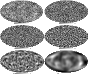	Figure 3: WMAP data and its wavelet transform on the sphere using five resolution levels (4 wavelet scales and the coarse scale). The sum of these five maps reproduces exactly the original data ( top left). Top: original data and the first wavelet scale. Middle: the second and third wavelet scales. Bottom: the fourth wavelet scale and the last smoothed array.
Open with DEXTER

Reconstruction

If the wavelet is the difference between two resolutions, Step 5 in the above UWTS algorithm can be replaced by the following simple subtraction w_j+1 = c_j - c_j+1. In this case, the reconstruction of an image from its wavelet coefficients ${\cal W} = \{w_1,\dots, w_{J}, c_{J}\}$ is straightforward:

$$c_{0}(\theta, \phi) = c_{J}(\theta, \phi) + \sum_{j=1}^J w_j(\theta, \phi).$$ (9)

This is the same reconstruction formula as in the à trous algorithm: the simple sum of all scales reproduces the original data. However, since the present decomposition is redundant, the procedure for reconstructing an image from its coefficients is not unique and this can profitably be used to impose additional constraints on the synthesis functions (e.g. smoothness, positivity) used in the reconstruction. Here for instance, using the relations:

$$\hat c_{j+1}(l,m) = \widehat H_{j} (l,m) \hat c_{j} (l,m)$$

$$\hat w_{j+1}(l,m) = \widehat G_{j} (l,m) \hat c_{j} (l,m)$$ (10)

a least squares estimate of c_j from c_j+1 and w_j+1 gives:

$$\hat{c}_{j} = \hat{c}_{j+1} {\widehat {\tilde H}}_{j} + \hat{w}_{j+1} {\widehat {\tilde G}}_{j}$$ (11)

where the conjugate filters ${\widehat {\tilde H}}_j$ and ${\widehat {\tilde G}}_j$ have the expression:

  

$${\widehat {\tilde H}}_j = \sqrt{\frac{4\pi}{2l+1} } {\hat {\tilde... ... {\widehat H}_{j}^* / (\mid {\widehat H}_{j}\mid^2 + \mid {\widehat G}_j\mid^2)$$ (12)

$${\widehat {\tilde G}}_j = \sqrt{\frac{4\pi}{2l+1} } {\hat {\tilde... ... {\widehat G}_{j}^* / (\mid {\widehat H}_j \mid^2 + \mid {\widehat G}_j \mid^2)$$ (13)

and the reconstruction algorithm is:

1.

Compute the B₃-spline scaling function and derive $\hat{\psi}$, $\hat h$, $\hat g$, $\hat{\tilde{h}}$, $\hat{\tilde{g}}$ numerically.

2.

Compute the corresponding Spherical Harmonics of the image at the low resolution c_J. We get ${\hat c}_J$.

3.

Set j to J-1. Iterate:

4.

Compute the Spherical Harmonics transform of the wavelet coefficients w_j+1 at scale j+1. We get $\hat{w}_{j+1}$.

5.

Multiply $\hat{c}_{j+1}$ by ${\widehat {\tilde H}}_j$.

6.

Multiply $\hat{w}_{j+1}$ by ${\widehat {\tilde G}}_j$.

7.

Add the results of steps 6 and 7. We get $\hat{c}_j$.

8.

j=j-1 and if $j \ge 0$, return to Step 4.

9.

Compute The inverse Spherical Harmonic transform of ${\hat c}_0$.

The synthesis low pass and high pass filters $\hat{\tilde{h}}$ and $\hat{\tilde{g}}$ are plotted in Fig. 2.

	Figure 4: Backprojection of a wavelet coefficient at different scales. Each map is obtained by setting all but one of the wavelet coefficients to zero, and applying an inverse wavelet transform. Depending on the scale and the position of the non zero wavelet coefficient, the reconstructed image presents an isotropic feature with a given size.
Open with DEXTER

Figure 3 shows the WMAP data (top left) and its undecimated wavelet decomposition on the sphere using five resolution levels. Figures 3 middle left, middle right and bottom left show respectively the four wavelet scales. Figure 3 bottom right shows the last smoothed array. Figure 4 shows the backprojection of a wavelet coefficient at different scales and positions.

2.2 Isotropic pyramidal wavelet transform on the sphere (PWTS)

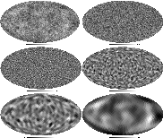Figure 5: WMAP data ( top left) and its pyramidal wavelet transform on the sphere using five resolution levels (4 wavelet scales and the coarse scale). The original map can be reconstructed exactly from the pyramidal wavelet coefficients. Top: original data and the first wavelet scale. Middle: the second and third wavelet scales. Bottom: the fourth wavelet scale and the last smoothed array. The number of pixels is divided by four at each resolution level, which can be helpful when the data set is large.

Open with DEXTER

In the previous algorithm, no downsampling is performed and each scale of the wavelet decomposition has the same number of pixels as the original data set. Therefore, the number of pixels in the decomposition is equal to the number of pixels in the data multiplied by the number of scales. For applications such as PLANCK data restoration, we may prefer to introduce some decimation in the decomposition so as to reduce the required memory size and the computation time. This can be done easily by using a specific property of the chosen scaling function. Indeed, since we are considering here a scaling function with an initial cut-off l_c in spherical harmonic multipole number l, and since the actual cut-off is reduced by a factor of two at each step, the number of significant spherical harmonic coefficients is then reduced by a factor of four after each convolution with the low pass filter h. Therefore, we need fewer pixels in the direct space when we compute the inverse spherical harmonic transform. Using the Healpix pixelization scheme (Górski et al. 2002), this can be done easily by dividing by 2 the nside parameter when resorting to the inverse spherical harmonic transform routine.

Figure 5 shows WMAP data (top left) and its pyramidal wavelet transform using five scales. As the scale number increases (i.e. the resolution decreases), the pixel size becomes larger. Figures 5 top right, middle left, middle right and bottom left show respectively the four wavelet scales. Figure 5 bottom right shows the last smoothed array.

	Figure 6: Flowgraph of the ridgelet transform on the sphere.
Open with DEXTER

   
3 Curvelet transform on the sphere (CTS)

3.1 Introduction

The 2D curvelet transform, proposed in Donoho & Duncan (2000), Starck et al. (2002a, 2003a) enables the directional analysis of an image in different scales. The fundamental property of the curvelet transform is to analyze the data with functions of length of about 2^-j/2 for the jth sub-band [2^j, 2^j+1] of the two dimensional wavelet transform. Following the implementation described in Starck et al. (2002a) and Starck et al. (2003a), the data first undergoes an isotropic undecimated wavelet transform (i.e. à trous algorithm). Each scale j is then decomposed into smoothly overlapping blocks of side-length B_j pixels in such a way that the overlap between two vertically adjacent blocks is a rectangular array of size $B_j \times B_j/2$. Finally, the ridgelet transform (Candès & Donoho 1999) is applied on each individual block which amounts to applying a 1-dimensional wavelet transform to the slices of its Radon transform. More details on the implementation of the digital curvelet transform can be found in Starck et al. (2002a, 2003a). It has been shown that the curvelet transform could be very useful for the detection and the discrimination of sources of non-Gaussianity in CMB (Starck et al. 2003b). The curvelet transform is also redundant, with a redundancy factor of 16J+1 whenever J scales are employed. Its complexity scales like that of the ridgelet transform that is as $O(n^2 \log_2n)$. This method is best for the detection of anisotropic structures and smooth curves and edges of different lengths.

3.2 Curvelets on the sphere

The curvelet transform on the sphere (CTS) can be similar to the 2D digital curvelet transform, but replacing the à trous algorithm by the isotropic wavelet transform on the sphere previously described. The CTS algorithm consists of the following three steps:

• Isotropic wavelet transform on the sphere.
• Partitioning. Each scale is decomposed into blocks of an appropriate scale (of side-length $\sim$2^-s), using the Healpix pixelization.
• Ridgelet analysis. Each square is analyzed via the discrete ridgelet transform.

Partitioning using the Healpix representation

The Healpix representation is a curvilinear partition of the sphere into quadrilateral pixels of exactly equal area but with varying shape. The base resolution divides the sphere into 12 quadrilateral faces of equal area placed on three rings around the poles and equator. Each face is subsequently divided into nside² pixels following a hierarchical quadrilateral tree structure. The geometry of the Healpix sampling grid makes it easy to partition a spherical map into blocks of a specified size 2ⁿ. We first extract the twelve base-resolution faces, and each face is then decomposed into overlapping blocks as in the 2D digital curvelet transform. With this scheme however, there is no overlapping between blocks belonging to different base-resolution faces. This may result in blocking effects for example in denoising experiments via non linear filtering. A simple way around this difficulty is to work with various rotations of the data with respect to the sampling grid.

Ridgelet transform

Once the partitioning is performed, the standard 2D ridgelet transform described in Starck et al. (2003a) is applied in each individual block:

1.

Compute the 2D Fourier transform.

2.

Extract lines going through the origin in the frequency plane.

3.

Compute the 1D inverse Fourier transform of each line. This achieves the Radon transform of the current block.

4.

Compute the 1D wavelet transform of the lines of the Radon transform.

The first three steps correspond to a Radon transform method called the linogram. Other implementations of the Radon transform, such as the Slant Stack Radon Transform (Donoho & Flesia 2002), can be used as well, as long as they offer an exact reconstruction.

Figure 6 shows the flowgraph of the ridgelet transform on the sphere and Fig. 7 shows the backprojection of a ridgelet coefficient at different scales and orientations.

	Figure 7: Backprojection of a ridgelet coefficient at different scales and orientations. Each map is obtained by setting all but one of the ridgelet coefficients to zero, and applying an inverse ridgelet transform. Depending on the scale and the position of the non zero ridgelet coefficient, the reconstructed image presents a feature with a given width and a given orientation.
Open with DEXTER

3.3 Algorithm

The curvelet transform algorithm on the sphere is as follows:

1.

Apply the isotropic wavelet transform on the sphere with J scales.

2.

Set the block size $B_1 = B_{\rm min}$.

3.

For $j = 1, \ldots, J$ do,

• partition the subband w_j with a block size B_j and apply the digital ridgelet transform to each block;
• if $j \mbox{ modulo } 2 = 1$ then B_j+1 = 2 B_j;
• else B_j+1 = B_j.

The sidelength of the localizing windows is doubled at every other dyadic subband, hence maintaining the fundamental property of the curvelet transform which says that elements of length about 2^-j/2 serve for the analysis and synthesis of the j-th subband [2^j, 2^j+1]. We used the default value $B_{\rm min} = 16$ pixels in our implementation. Figure 8 gives an overview of the organization of the algorithm. Figure 9 shows the backprojection of curvelet coefficients at different scales and orientations.

	Figure 8: Flowgraph of the curvelet transform on the sphere.
Open with DEXTER

3.4 Pyramidal curvelet transform on the sphere (PCTS)

The CTS is very redundant, which may be a problem in handling huge data sets such as the future PLANCK data. The redundancy can be reduced by substituting, in the curvelet transform algorithm, the pyramidal wavelet transform to the undecimated wavelet transform. The second step which consists in applying the ridgelet transform on the wavelet scale is unchanged. The pyramidal curvelet transform algorithm is:

1.

Apply the pyramidal wavelet transform on the sphere with J scales.

2.

Set the block size $B_1 = B_{\rm min}$.

3.

For $j = 1, \ldots, J$ do,

• partition the subband w_j with a block size B_j and apply the digital ridgelet transform to each block,
• if $j \mbox{ modulo } 2 = 2$ then B_j+1 = B_j / 2,
• else B_j+1 = B_j.

In the next section, we show how the pyramidal curvelet transform can be used for image filtering.

   
4 Filtering

4.1 Hard thresholding

Wavelets and Curvelets have been used successfully in image denoising via non-linear filtering or thresholding methods (Starck & Murtagh 2002; Starck et al. 2002a). Hard thresholding, for instance, consists in setting all insignificant coefficients (i.e. coefficients with an absolute value below a given threshold) to zero. In practice, we need to estimate the noise standard deviation $\sigma_j$ in each band jand a wavelet (or curvelet) coefficient w_j is significant if $\mid w_j \mid ~ > k \sigma_j$, where k is a user-defined parameter, typically chosen between 3 and 5. The $\sigma_j$ estimation in band j can be derived from simulations (Starck & Murtagh 2002). Denoting as D the noisy data and $\delta$ the thresholding operator, the filtered data $\tilde D$ are obtained by:

$${\tilde D} = {\cal R} \delta( {\cal T} D)$$ (14)

where ${\cal T}$ is the wavelet (resp. curvelet) transform operator and ${\cal R}$ is the wavelet (resp. curvelet) reconstruction operator.

	Figure 9: Backprojection of a curvelet coefficient at different scales and orientations. Each map is obtained by setting all but one of the curvelet coefficients to zero, and applying an inverse curvelet transform. Depending on the scale and the position of the non zero curvelet coefficient, the reconstructed image presents a feature with a given width, length and orientation.
Open with DEXTER

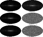	Figure 10: Denoising. Upper left and right: simulated synchrotron image and same image with an additive Gaussian noise (i.e. simulated data). Middle: pyramidal wavelet filtering and residual. Bottom: pyramidal curvelet filtering and residual. On such data, displaying very anisotropic features, the residual with curvelet denoising is cleaner than with the wavelet denoising.
Open with DEXTER

Figure 10 describes the setting and the results of a simulated denoising experiment: upper left, the original simulated map of the synchrotron emission (renormalized between 0 and 255); upper right, the same image plus additive Gaussian noise ($\sigma=5$); middle, the pyramidal wavelet filtered image and the residual (i.e. noisy data minus filtered data); bottom, the pyramidal curvelet transform filtered image and the residual. A $5 \sigma_j$ detection threshold was used in both cases. On such data, displaying very anisotropic features, using curvelets produces better results than the wavelets.

4.2 The combined filtering method on the sphere

	Figure 11: Denoising. Combined Filtering Method (pyramidal wavelet and pyramidal curvelet) and residual.
Open with DEXTER

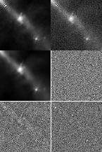	Figure 12: Combined Filtering Method, face 6 in the Healpix representation of the image shown in Fig. 11. From top to bottom and left to right, respectively the a) original image face, b) the noisy image, c) the combined filtered image, d) the combined filtering residual, e) the wavelet filtering residual and f) the curvelet filtering residual.
Open with DEXTER

The residual images for both the wavelet and curvelet transforms shown in Fig. 10 show that wavelets do not restore long features with high fidelity while curvelets are seriously challenged by isotropic or small features. Each transform has its own area of expertise and this complementarity is of great potential. The Combined Filtering Method (CFM) (Starck et al. 2001) allows us to benefit from the advantages of both transforms. This iterative method detects the significant coefficients in both the wavelet domain and the curvelet domain and guarantees that the reconstructed map will take into account any pattern detected as significant by either of the transforms. A full description of the algorithm is given in Appendix A. Figure 11 shows the CFM denoised image and its residual. Figure 12 shows one face (face 6) of the following Healpix images: upper left, original image; upper right, noisy image; middle left, restored image after denoising by the combined transform; middle right, the residual; bottom left and right, the residual using respectively the curvelet and the wavelet denoising method. The results are reported in Table 1. The residual is much better when the combined filtering is applied, and no feature can be detected any longer by eye in the residual. Neither with the wavelet filtering nor with the curvelet filtering could such a clean residual be obtained.

   
5 Wavelets on the sphere and independent component analysis

5.1 Introduction

Blind Source Separation (BSS) is a problem that occurs in multi-dimensional data processing. The goal is to recover unobserved signals, images or sources S from mixtures X of these sources observed typically at the output of an array of m sensors. A simple mixture model would be linear and instantaneous with additive noise as in:

 

X = A S + N (15)

where X, S and N are random vectors of respective sizes $m \times 1$, $n\times 1$ and $m \times 1$, and A is an $m\times n$ matrix. Multiplying S by A linearly mixes the n sources resulting in m observed mixture processes corrupted by additive instrumental Gaussian noise N. Independent Component Analysis methods were developed to solve the BSS problem, i.e. given a batch of T observed samples of X, estimate A and S, relying mostly on the statistical independence of the source processes.

Algorithms for blind component separation and mixing matrix estimation depend on the a priori model used for the probability distributions of the sources (Cardoso 2001) although rather coarse assumptions can be made (Cardoso 1998; Hyvärinen et al. 2001). In a first set of techniques, source separation is achieved in a noise-less setting, based on the non-Gaussianity of all but possibly one of the components. Most mainstream ICA techniques belong to this category: JADE (Cardoso 1999), FastICA, Infomax (Hyvärinen et al. 2001). In a second set of blind techniques, the components are modeled as Gaussian processes and, in a given representation (Fourier, wavelet, etc.), separation requires that the sources have diverse, i.e. non proportional, variance profiles. The Spectral Matching ICA method (SMICA) (Delabrouille et al. 2003; Moudden et al. 2005) considers in this sense the case of mixed stationary Gaussian components in a noisy context: moving to a Fourier representation, the point is that colored components can be separated based on the diversity of their power spectra.

5.2 SMICA: from Fourier to wavelets

Table 1: Table of error standard deviations and SNR values after filtering the synchrotron noisy map (Gaussian white noise - sigma = 5 ) by the wavelet, the curvelet and the combined filtering method. Images are available at http://jstarck.free.fr/mrs.html.

SMICA, which was designed to address some of the general problems raised by Cosmic Microwave Background data analysis, has already shown significant success for CMB spectral estimation in multidetector experiments (Delabrouille et al. 2003; Patanchon et al. 2004). However, SMICA suffers from the non locality of the Fourier transform which has undesired effects when dealing with non-stationary components or noise, or with incomplete data maps. The latter is a common issue in astrophysical data analysis: either the instrument scanned only a fraction of the sky or some regions of the sky were masked due to localized strong astrophysical sources of contamination (compact radio-sources or galaxies, strong emitting regions in the galactic plane). A simple way to overcome these effects is to move instead to a wavelet representation so as to benefit from the localization property of wavelet filters, which leads to wSMICA (Moudden et al. 2005). The wSMICA method uses an undecimated à trous algorithm with the cubic box-spline (Starck & Murtagh 2002) as the scaling function. This transform has several favorable properties for astrophysical data analysis. In particular, it is a shift invariant transform, the wavelet coefficient maps on each scale are the same size as the initial image, and the wavelet and scaling functions have small compact supports in the initial representation. All of these allow missing patches in the data maps to be handled easily.

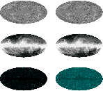Figure 13: Left: zero mean templates for CMB ( $\sigma = 4.17\times 10^{-5}$), galactic dust ( $\sigma = 8.61\times 10^{-6}$) and SZ ( $\sigma = 3.32\times 10^{-6}$) used in the experiment described in Sect. 5.4. The standard deviations given are for the region outside the galactic mask. The maps on the right were estimated using wSMICA and scalewise Wiener filtering as is explained in Appendix B. Map reconstruction using Wiener filtering clearly is optimal only in front of stationary Gaussian processes. For non Gaussian maps, such as given by the Sunyaev Zel'dovich effect, better reconstruction can be expected from non linear methods. The different maps are drawn here in different color scales to enhance structures and ease visual comparisons.

Open with DEXTER

Using this wavelet transform algorithm, the multichannel data X is decomposed into J detail maps X_j^w and a smooth approximation map X_J+1^w over a dyadic resolution scale. Since applying a wavelet transform on (15) does not affect the mixing matrix A, the covariance matrix of the observations at scale j is still structured as

$$R_w^X(j) = A R_w^S(j) A^{\dagger} + R_w^N(j)$$ (16)

where R_w^S(j) and R_w^N(j) are the diagonal spectral covariance matrices in the wavelet representation of S and N respectively. It was shown (Moudden et al. 2005) that replacing in the SMICA method the covariance matrices derived from the Fourier coefficients by the covariance matrices derived from wavelet coefficients leads to much better results when the data are incomplete. This is due to the fact that the wavelet filter response on scale j is short enough compared to data size and gap widths and most of the samples in the filtered signal then remain unaffected by the presence of gaps. Using these samples exclusively yields an estimated covariance matrix $\widehat{R}_w^X(j)$ which is not biased by the missing data.

Table 2: Entries of A, the mixing matrix used in our simulations.

5.3 SMICA on the sphere: from spherical harmonics to wavelets on the sphere (wSMICA-S)

Table 3: Nominal noise standard deviations in the six channels of the Planck HFI.

Extending SMICA to deal with multichannel data mapped to the sphere is straightforward (Delabrouille et al. 2003). The idea is simply to substitute the spherical harmonics transform for the Fourier transform used in the SMICA method. Then, data covariance matrices are estimated in this representation over intervals in multipole number l. However SMICA on spherical maps still suffers from the non locality of the spherical harmonics transform whenever the data to be processed is non stationary, incomplete, or partly masked.

Moving to a wavelet representation allows one to overcome these effects: wSMICA can be easily implemented for data mapped to the sphere by substituting the UWTS described in Sect. 2 to the undecimated à trous algorithm used in the previous section. In the linear mixture model (15), X now stands for an array of observed spherical maps, S is now an array of spherical source maps to be recovered and N is an array of spherical noise maps. The mixing matrix A achieves a pixelwise linear mixing of the source maps. Applying the above UWTS on both sides of (15) does not affect the mixing matrix A so that, assuming independent source and noise processes, the covariance matrix of the observations at scale j is again structured as in (16). Source separation follows from minimizing the covariance matching criterion (23) in this spherical wavelet representation. A full description is given in Appendix B.

   
5.4 Experiments

As an application of wSMICA on the sphere, we consider here the problem of CMB data analysis but in the special case where the use of a galactic mask is a cause of non-stationarity which impairs the use of the spherical harmonics transform.

The simulated CMB, galactic dust and Sunyaev Zel'dovich (SZ) maps used, shown on the left-hand side of Fig. 13, were obtained as described in Delabrouille et al. (2003). The problem of instrumental point spread functions is not addressed here, and all maps are assumed to have the same resolution. The high level foreground emission from the galactic plane region was removed using the Kp2 mask from the WMAP team website. These three incomplete maps were mixed using the matrix in Table 2, in order to simulate observations in the six channels of the Planck high frequency instrument (HFI).

Gaussian instrumental noise was added in each channel according to model (15). The relative noise standard deviations between channels were set according to the nominal values of the Planck HFI given in Table 3.

The synthetic observations were decomposed into six scales using the isotropic UWTS and wSMICA was used to obtain estimates of the mixing matrix and of the initial source templates. The resulting component maps estimated using wSMICA, for nominal noise levels, are shown on the right-hand side of Fig. 13 where the quality of the reconstruction can be visually assessed by comparison to the initial components. The component separation was also performed with SMICA based on Fourier statistics computed in the same six dyadic bands imposed by our choice of wavelet transform, and with JADE. In Fig. 14, the performances of SMICA, wSMICA and JADE are compared in the particular case of CMB map estimation, in terms of the relative standard deviation of the reconstruction error, MQE, defined by

$$MQE = \frac{\mathbf{std} ( CMB(\vartheta, \varphi) - \alpha \... ...rtheta, \varphi) )}{\mathbf{std} ( CMB(\vartheta, \varphi) ) }$$ (17)

where std stands for empirical standard deviation (obviously computed outside the masked regions), and $\alpha$ is a linear regression coefficient estimated in the least squares sense. As expected, since it is meant to be used in a noiseless setting, JADE performs well when the noise is very low. However, as the noise level increases, its performance degrades quite rapidly compared to the covariance matching methods. Further, these results clearly show that using wavelet-based covariance matrices provides a simple and efficient way to treat the effects of gaps on the performance of source separation using statistics based on the non local Fourier representation.

	Figure 14: Relative reconstruction error defined by (17) of the CMB component map using SMICA, wSMICA and JADE as a function of the instrumental noise level in dB relative to the nominal values in Table 3. The zero dB noise level corresponds to the expected noise in the future PLANCK mission.
Open with DEXTER

6 Conclusion

We have introduced new multiscale decompositions on the sphere, the wavelet transform, the ridgelet transform and the curvelet transform. It was shown in Starck et al. (2004) that combining the statistics of wavelet coefficients and curvelet coefficients of flat maps leads to a powerful analysis of the non-Gaussianity in the CMB. Using the new decompositions proposed here, it is now possible to perform such a study on data mapped to the sphere such as from the WMAP or PLANCK experiments. For the denoising application, we have shown that the Combined Filtering Method allows us to significantly improve the result compared to a standard hard thresholding in a given transformation. Using the isotropic UWTS and statistics in this representation also allows us to properly treat incomplete or non-stationary data on the sphere which cannot be done in the non-local Fourier representation. This is clearly illustrated by the results obtained with wSMICA which achieves component separation in the wavelet domain thus reducing the negative impact that gaps have on the performance of source separation using the initial SMICA algorithm in the spherical harmonics representation. Further results are available at http://jstarck.free.fr/mrs.hmtl

as well as information about the IDL code for the described transformations based on the Healpix package (Górski et al. 2002).

Acknowledgements

We wish to thank David Donoho, Jacques Delabrouille, Jean-François Cardoso and Vicent Martinez for useful discussions.

References

• Aghanim, N., & Forni, O. 1999, A&A, 347, 409 [NASA ADS]
• Antoine, J., Demanet, L., Jacques, L., & Vandergheynst, P. 2002, Appl. Comput. Harmon. Anal., 13, 177 [CrossRef]
• Antoine, J.-P. 1999, in Wavelets in Physics, 23
• Barreiro, R. B., Martínez-González, E., & Sanz, J. L. 2001, MNRAS, 322, 411 [NASA ADS] [CrossRef]
• Bogdanova, I., Vandergheynst, P., Antoine, J.-P., Jacques, L., & Mrovidone, M. 2005, Applied and Computational Harmonic Analysis, in press (In the text)
• Candès, E., & Donoho, D. 1999, Philosophical Transactions of the Royal Society of London A, 357, 2495 [NASA ADS] (In the text)
• Cardoso, J.-F. 1998, Proceedings of the IEEE. Special issue on blind identification and estimation, 9(10), 2009
• Cardoso, J.-F. 1999, Neural Computation, 11(1), 157 (In the text)
• Cardoso, J.-F. 2001, in Proc. ICA 2001, San Diego (In the text)
• Cayón, L., Sanz, J. L., Martínez-González, E., et al. 2001, MNRAS, 326, 1243 [NASA ADS] [CrossRef]
• Delabrouille, J., Cardoso, J.-F., & Patanchon, G. 2003, MNRAS, 346, 1089 [NASA ADS] [CrossRef],
• Donoho, D., & Duncan, M. 2000, in Proc. Aerosense 2000, Wavelet Applications VII, ed. H. Szu, M. Vetterli, W. Campbell, & J. Buss, SPIE, 4056, 12
• Donoho, D., & Flesia, A. 2002, in Beyond Wavelets, ed. J. Schmeidler, & G. Welland (Academic Press) (In the text)
• Escalera, E., & MacGillivray, H. T. 1995, A&A, 298, 1 [NASA ADS]
• Fang, L.-Z., & Feng, L.-l. 2000, ApJ, 539, 5 [NASA ADS] [CrossRef] (In the text)
• Freeden, W., & Schneider, F. 1998, Inverse Problems, 14, 225 [NASA ADS] [CrossRef]
• Freeden, W., & Windheuser, U. 1997, Applied and Computational Harmonic Analysis, 4, 1 [CrossRef]
• Górski, K. M., Banday, A. J., Hivon, E., & Wandelt, B. D. 2002, in ASP Conf. Ser., 107 (In the text)
• Holschneider, M. 1996, J. Math. Phys., 37(8), 4156
• Hyvärinen, A., Karhunen, J., & Oja, E. 2001, Independent Component Analysis (New York: John Wiley), 481
• Martinez, V., Starck, J.-L., Saar, E., et al. 2005, ApJ, 634, 744 [NASA ADS] [CrossRef]
• McEwen, J. D., Hobson, M. P., Lasenby, A. N., & Mortlock, D. J. 2004, MNRAS, submitted
• Moudden, Y., Cardoso, J.-F., Starck, J.-L., & Delabrouille, J. 2005, Eurasip Journal, 15, 2437 (In the text)
• Mukherjee, P., & Wang, Y. 2003, ApJ, 599, 1 [NASA ADS] [CrossRef] (In the text)
• Patanchon, G., Cardoso, J. F., Delabrouille, J., & Vielva, P. 2004, MNRAS, submitted
• Rocha, G., Cayón, L., Bowen, R., et al. 2004, MNRAS, 351, 769 [NASA ADS] [CrossRef] (In the text)
• Romeo, A. B., Horellou, C., & Bergh, J. 2003, MNRAS, 342, 337 [NASA ADS] [CrossRef]
• Romeo, A. B., Horellou, C., & Bergh, J. 2004, MNRAS, 354, 1208 [NASA ADS] [CrossRef]
• Schröder, P., & Sweldens, W. 1995, Computer Graphics Proceedings (SIGGRAPH 95), 161
• Slezak, E., de Lapparent, V., & Bijaoui, A. 1993, ApJ, 409, 517 [NASA ADS] [CrossRef]
• Starck, J.-L., & Murtagh, F. 2002, Astron. Image Data Analysis (Springer-Verlag) (In the text)
• Starck, J.-L., Bijaoui, A., Lopez, B., & Perrier, C. 1994, A&A, 283, 349 [NASA ADS] (In the text)
• Starck, J.-L., Murtagh, F., & Bijaoui, A. 1998, Image Processing and Data Analysis: The Multiscale Approach (Cambridge University Press) (In the text)
• Starck, J.-L., Donoho, D. L., & Candès, E. J. 2001, in Wavelets: Applications in Signal and Image Processing IX, ed. A. F. Laine, M. A. Unser, & A. Aldroubi, Proc. SPIE, 4478, 9 (In the text)
• Starck, J.-L., Candès, E., & Donoho, D. 2002a, IEEE Trans. Image Processing, 11(6), 131
• Starck, J.-L., Pantin, E., & Murtagh, F. 2002b, ASP, 114, 1051 [NASA ADS] (In the text)
• Starck, J.-L., Candes, E., & d Donoho, D. 2003a, A&A, 398, 785 [EDP Sciences] [NASA ADS] [CrossRef] (In the text)
• Starck, J.-L., Murtagh, F., Candes, E., & Donoho, D. 2003b, IEEE Trans. Image Processing, 12(6), 706 (In the text)
• Starck, J.-L., Aghanim, N., & Forni, O. 2004, ApJ, 416, 9
• Starck, J.-L., Martinez, V., Donoho, D., et al. 2005a, EURASIP JASP, 15, 2455
• Starck, J.-L., Pires, S., & Refrégier, A. 2005b, A&A, submitted (In the text)
• Tenorio, L., Jaffe, A. H., Hanany, S., & Lineweaver, C. H. 1999, MNRAS, 310, 823 [NASA ADS] [CrossRef]
• Vielva, P., Martínez-González, E., Barreiro, R. B., Sanz, J. L., & Cayón, L. 2004, ApJ, 609, 22 [NASA ADS] [CrossRef]
• Wiaux, Y., Jacques, L., & Vandergheynst, P. 2005, ApJ, 632, 15 [NASA ADS] [CrossRef]
• Yamada, I. 2001, in Inherently Parallel Algorithms in Feasibility and Optimization and Their Applications, ed. D. Butnariu, Y. Censor, & S. Reich (Elsevier) (In the text)

 

  Online Material

Appendix A: The combined filtering method

In general, suppose that we are given K linear transforms $T_1, \ldots, T_K$ and let $\alpha_k$ be the coefficient sequence of an object x after applying the transform T_k, i.e. $\alpha_k = T_k x$. We will assume that for each transform T_k, a reconstruction rule is available that we will denote by T^-1_k, although this is clearly an abuse of notation. T will denote the block diagonal matrix with T_k as building blocks and $\alpha$ the amalgamation of the $\alpha_k$.

A hard thresholding rule associated with the transform T_k synthesizes an estimate $\tilde{s}_k$ via the formula

$$\tilde{s}_k = T_k^{-1} \delta(\alpha_k)$$ (18)

where $\delta$ is a rule that sets to zero all the coordinates of $\alpha_k$ whose absolute value falls below a given sequence of thresholds (such coordinates are said to be non-significant).

Given data y of the form $y = s + \sigma z$, where s is the image we wish to recover and z is standard white noise, we propose to solve the following optimization problem (Starck et al. 2001):

$$\min \Vert T\tilde{s}\Vert _{\ell_1}, \quad \mbox{subject to} \quad s \in C,$$ (19)

where C is the set of vectors $\tilde{s}$ that obey the linear constraints

$$\left\{ \begin{array}{ll} \tilde{s} \ge 0, \\ \vert T\tilde{s} - Ty\vert \le e; \end{array} \right.$$ (20)

here, the second inequality constraint only concerns the set of significant coefficients, i.e. those indices $\mu$ such that $\alpha_\mu = (Ty)_\mu$ exceeds (in absolute value) a threshold $t_\mu$. Given a vector of tolerance $(e_\mu)$, we seek a solution whose coefficients $(T\tilde{s})_\mu$ are within $e_\mu$ of the noisy empirical $\alpha_\mu$. Think of $\alpha_\mu$ as being given by

$$y = \langle y, \varphi_\mu \rangle,$$

so that $\alpha_\mu$ is normally distributed with mean $\langle f, \varphi_\mu \rangle$ and variance $\sigma^2_\mu = \sigma^2 \Vert\varphi_\mu\Vert^2_2$. In practice, the threshold values range typically between three and four times the noise level $\sigma_\mu$and in our experiments we will put $e_\mu = \sigma_\mu/2$. In short, our constraints guarantee that the reconstruction will take into account any pattern detected as significant by any of the K transforms.

The minimization method

We propose to solve (19) using the method of hybrid steepest descent (HSD) (Yamada 2001). HSD consists of building the sequence

$$s^{n+1} = P(s^{n}) - \lambda_{n+1} \nabla_J(P(s^{n}));$$ (21)

Here, P is the $\ell_2$ projection operator onto the feasible set C, $\nabla_J$ is the gradient of Eq. (19), and $(\lambda_{n})_{n \ge 1}$ is a sequence obeying $(\lambda_{n})_{n\ge 1} \in [0,1]$ and $\lim_{ n \rightarrow + \infty } \lambda_{n} = 0$.

The combined filtering algorithm is:

1.

Initialize $L_{\max} = 1$, the number of iterations N_i, and $\delta_{\lambda} = \frac{L_{\max}}{N_i}$.

2.

Estimate the noise standard deviation $\sigma$, and set $e_k = \frac{\sigma}{2}$.

3.

For k = 1, .., K calculate the transform: $\alpha^{(s)}_k = T_k s$.

4.

Set $\lambda = L_{\max}$, n = 0, and $\tilde s^{n}$ to 0.

5.

While $\lambda >= 0$ do

• $u = \tilde s^{n}$.
• For k = 1, .., K do
  • Calculate the transform $\alpha_{k} = T_k u$.
  • For all coefficients $\alpha_{k,l}$ do
    • Calculate the residual $r_{k,l} = \alpha^{(s)}_{k,l} - \alpha_{k,l}$,

    • if $\alpha^{(s)}_{k,l}$ is significant and $\mid r_{k,l} \mid > e_{k,l}$ then $\alpha_{k,l} = \alpha^{(s)}_{k,l}$,
    • $\alpha_{k,l} = sgn(\alpha_{k,l}) ( \mid \alpha_{k,l} \mid - \lambda)_{+}$.
  • $u = T_k^{-1} \alpha_{k}$.
• Threshold negative values in u and $\tilde s^{n+1} = u$.
• n = n + 1, $\lambda = \lambda - \delta_{\lambda}$, and goto 5.

Appendix B: SMICA in the spherical wavelet representation (wSMICA-S)

A detailed derivation of SMICA and wSMICA can be found in Delabrouille et al. (2003) and Moudden et al. (2005). Details are given here showing how the Isotropic Undecimated Wavelet Transform on the Sphere described in Sect. 2 above can be used to extend SMICA to work in the wavelet domain on spherical data maps. We will refer to this extension as wSMICA-S.

wSMICA-S objective function

In the linear mixture model (15), X stands for an array of observed spherical maps, S is an array of spherical source maps to be recovered and N is an array of spherical noise maps. The mixing matrix A achieves a pixelwise linear mixing of the source maps. The observations are assumed to have zero mean. Applying the above UWTS on both sides of (15) does not affect the mixing matrix A so that, assuming independent source and noise processes, the covariance matrix of the observations at scale j is still structured as

$$R_w^X(j) = A R_w^S(j) A^{\dagger} + R_w^N(j)$$ (22)

where R_w^S(j) and R_w^N(j) are the model diagonal spectral covariance matrices in the wavelet representation of S and N respectively. Provided estimates $\widehat{R}_w^X(j)$ of R_w^X(j) can be obtained from the data, our wavelet-based version of SMICA consists in minimizing the wSMICA-S criterion:

$$\Phi (\theta) = \sum _{j=1}^{J+1} \alpha_j \mathcal{D} \lef... ...idehat{R}_w^X(j), ~ A R_w^S(j) A^{\dagger} + R_w^N(j) \right)$$ (23)

for some reasonable choice of the weights $\alpha_j$ and of the matrix mismatch measure $\mathcal{D}$, with respect to the full set of parameters $\theta = (A,R_w^S(j), R_w^N(j) )$ or a subset thereof. As discussed in Delabrouille et al. (2003) and Moudden et al. (2005), a good choice for $\mathcal{D}$ is

$$\mathcal{D}_{KL} (R_1, R_2 ) = \frac{1}{2} \Big( {\rm tr} (R_1R_2^{-1}) - \log\det (R_1R_2^{-1}) - m \Big)$$ (24)

which is the Kullback-Leibler divergence between two m-variate zero-mean Gaussian distributions with covariance matrices R₁ and R₂. With this mismatch measure, the wSMICA-S criterion is shown to be related to the likelihood of the data in a Gaussian model. We can resort to the EM algorithm to minimize (23).

In dealing with non stationary data or incomplete data, an attractive feature of wavelet filters over the spherical harmonic transform is that they are well localized in the initial representation. Provided the wavelet filter response on scale j is short enough compared to data size and gap widths, most of the samples in the filtered signal will then be unaffected by the presence of gaps. Using exclusively these samples yields an estimated covariance matrix $\widehat{R}_w^X(j)$ which is not biased by the missing data. Writing the wavelet decomposition on J scales of X as

$$X(\vartheta, \varphi) = X_{J+1}^w (\vartheta, \varphi) + \sum_{j=1}^{J} X_{j}^w(\vartheta, \varphi)$$ (25)

and denoting l_j the size of the set $\mathcal{M}_j$ of wavelet coefficients unaffected by the gaps at scale j, the wavelet covariances are simply estimated using

$$\widehat{R}_w^X (j) = \frac{1}{l_j } \sum_{t \in \mathcal{M}_... ...theta_t, \varphi_t )X_j^w( \vartheta_t, \varphi_t ) ^\dagger .$$ (26)

The weights in the spectral mismatch (23) should be chosen to reflect the variability of the estimate of the corresponding covariance matrix. Since wSMICA-S uses wavelet filters with only limited overlap, in the case of complete data maps we follow the derivation in Delabrouille et al. (2003) and take $\alpha_j$ to be proportional to the number of spherical harmonic modes in the spectral domain covered at scale j. In the case of data with gaps, we must further take into account that only a fraction $\beta_j$ of the wavelet coefficients are unaffected so that the $\alpha_j$ should be modified in the same ratio.

Source map estimation

As a result of applying wSMICA-S, power densities in each scale are estimated for the sources and detector noise along with the estimated mixing matrix. These are used in reconstructing the source maps via Wiener filtering in each scale: a coefficient $X_{j}^w(\vartheta, \varphi)$ is used to reconstruct the maps according to

 

$$\widehat{S}_{j}^w(\vartheta, \varphi) = \big(\widehat{A} ^\dagger... ...{-1} \widehat{A} ^\dagger\widehat{R}_w^N( j) ^{-1} X_{j}^w(\vartheta, \varphi).$$ (27)

In the limiting case where noise is small compared to signal components, this filter reduces to

$$\widehat{S}_{j}^w(\vartheta, \varphi) = (\widehat{A} ^\dagg... ...^\dagger\widehat{R}_w^N( j) ^{-1} X_{j}^w(\vartheta, \varphi).$$ (28)

Clearly, the above Wiener filter is optimal only for stationary Gaussian processes. For non Gaussian maps, such as given by the Sunyaev Zel'dovich effect, better reconstruction can be expected from non linear methods.