A&A 446, 635-641 (2006)
DOI: 10.1051/0004-6361:20053187
L. Bigot1 - P. Kervella2 - F. Thévenin1 - D. Ségransan3
1 - Département Cassiopée, UMR 6202, Observatoire de la
Côte d'Azur, BP 4229, 06304 Nice Cedex 4, France
2 - LESIA, UMR
8109, Observatoire de Paris-Meudon, 5 place Jules Janssen, 92195
Meudon Cedex, France
3 - Observatoire de Genève, 1290
Sauverny, Switzerland
Received 4 April 2005 / Accepted 12 September 2005
Abstract
For the nearby dwarf star ![]() Cen B (K1 V), we
present limb-darkening predictions from a 3D hydrodynamical
radiative transfer model of its atmosphere.
We first compared the results of this model to a standard Kurucz's
atmosphere. Then we used both predictions to fit the new
interferometric visibility measurements of
Cen B (K1 V), we
present limb-darkening predictions from a 3D hydrodynamical
radiative transfer model of its atmosphere.
We first compared the results of this model to a standard Kurucz's
atmosphere. Then we used both predictions to fit the new
interferometric visibility measurements of ![]() Cen B obtained
with the VINCI instrument of the VLT Interferometer.
Part of these new visibility measurements were obtained in the
second lobe of the visibility function, which is sensitive to
stellar limb-darkening.
The best agreement is found for the 3D atmosphere limb-darkening
model and a limb-darkened angular diameter of
Cen B obtained
with the VINCI instrument of the VLT Interferometer.
Part of these new visibility measurements were obtained in the
second lobe of the visibility function, which is sensitive to
stellar limb-darkening.
The best agreement is found for the 3D atmosphere limb-darkening
model and a limb-darkened angular diameter of
![]() mas, corresponding to a linear radius of
mas, corresponding to a linear radius of
![]() (assuming
(assuming
![]() mas).
Our new linear radius agrees well with the asteroseismic value
predicted by Thévenin et al. (2002, A&A, 392, L9). In view of future
observations of this star with the VLTI/AMBER instrument, we also
present limb-darkening predictions in the J, H, and K bands.
mas).
Our new linear radius agrees well with the asteroseismic value
predicted by Thévenin et al. (2002, A&A, 392, L9). In view of future
observations of this star with the VLTI/AMBER instrument, we also
present limb-darkening predictions in the J, H, and K bands.
Key words: instrumentation: interferometers - stars: atmospheres
Limb-darkening (hereafter LD) is a well-known effect in stellar
physics. Its manifestation is a non-uniform brightness of the
disk, whose edges appear fainter than the center. This effect
occurs because of the decrease in the source function outwards in
the atmosphere. The disk center then shows deeper and warmer layers,
whereas the edges show higher and cooler material. This means that
analysis of the intensity
![]() at different
latitudinal angles
at different
latitudinal angles
![]() provides information on the
temperature variation with depth in the external layers of the star.
This is therefore an excellent constraint for testing atmospheric
models, to validate or invalidate assumptions used to derive these
models (like NLTE/LTE), and to provide suggestions for improving the
input physics (equation-of-state and/or opacities in particular).
The center-to-limb variation of the Sun has been known for many
years and been measured for numerous
provides information on the
temperature variation with depth in the external layers of the star.
This is therefore an excellent constraint for testing atmospheric
models, to validate or invalidate assumptions used to derive these
models (like NLTE/LTE), and to provide suggestions for improving the
input physics (equation-of-state and/or opacities in particular).
The center-to-limb variation of the Sun has been known for many
years and been measured for numerous ![]() and
and ![]() (e.g.
Pierce & Slaughter 1977; Neckel & Labs 1994; Hestroffer &
Magnan 1998) leading to a plethora of theoretical
works that have improved our knowledge of the external layers of the Sun.
(e.g.
Pierce & Slaughter 1977; Neckel & Labs 1994; Hestroffer &
Magnan 1998) leading to a plethora of theoretical
works that have improved our knowledge of the external layers of the Sun.
Traditionally, analysis of solar and stellar LD is made by adopting
an approximated law for
![]() ,
generally a polynomial
expansion in
,
generally a polynomial
expansion in ![]() that are either linear or non-linear (see e.g.
Claret 2000, for recent developments) and with
coefficients determined from 1D atmospheric models, like ATLAS
(Kurucz 1992) or Phoenix
(Hauschildt 1999). However, in spite of the detailed
physics included in these codes, their 1D nature is a limitation for
deriving realistic emergent intensities. Indeed, these codes contain
free parameters, like the well-known mixing length parameter, which
are injected artificially in order to reproduce the properties of
the turbulent convection at the stellar surface. As a consequence,
the comparison between these 1D models and observations depends on
the input parameters, which thereby creates an important source of
uncertainties. Moreover, convection is by nature a 3D process. Its
manifestation is the presence of bright granules and dark
intergranular lanes. Reducing it to a 1D process, i.e. ignoring
horizontal flows and temperature inhomogeneities, changes the
pressure scale height, the location of the surface, and therefore
also the emergent intensity (see e.g. Allende-Prieto et al.
2004; and Asplund et al. 2000a, for a
comparison of multi-dimensional simulations).
that are either linear or non-linear (see e.g.
Claret 2000, for recent developments) and with
coefficients determined from 1D atmospheric models, like ATLAS
(Kurucz 1992) or Phoenix
(Hauschildt 1999). However, in spite of the detailed
physics included in these codes, their 1D nature is a limitation for
deriving realistic emergent intensities. Indeed, these codes contain
free parameters, like the well-known mixing length parameter, which
are injected artificially in order to reproduce the properties of
the turbulent convection at the stellar surface. As a consequence,
the comparison between these 1D models and observations depends on
the input parameters, which thereby creates an important source of
uncertainties. Moreover, convection is by nature a 3D process. Its
manifestation is the presence of bright granules and dark
intergranular lanes. Reducing it to a 1D process, i.e. ignoring
horizontal flows and temperature inhomogeneities, changes the
pressure scale height, the location of the surface, and therefore
also the emergent intensity (see e.g. Allende-Prieto et al.
2004; and Asplund et al. 2000a, for a
comparison of multi-dimensional simulations).
The precise measurements of the center-to-limb variation achieved nowadays require realistic stellar atmospheric models that take all the complexity of the stellar surface into account, and motivates the use of the new generation of 3D radiative hydrodynamical (hereafter RHD) simulations.
In this paper we propose a study of ![]() Cen B
(HD128621), a nearby K1V dwarf star. It is part of a
visual triple star system whose brightest component,
Cen B
(HD128621), a nearby K1V dwarf star. It is part of a
visual triple star system whose brightest component, ![]() Cen A
(HD128620), is a G2V dwarf. Both theoretical and
observational considerations motivated the selection of this star
in the present work. From the interferometric point of view, the
proximity (1.3 pc) of the star is a rare opportunity for
interferometric measurements, since most of the nearby dwarfs have
angular diameters that are too small to be measured. Our interest in this
star grew recently since our new measurements provided data points
in the second lobe of the visibility function, which is sensitive to
the LD of the star. From a theoretical point of view, this star is
important for various reasons. In particular, recent detection of
solar-like oscillations in
Cen A
(HD128620), is a G2V dwarf. Both theoretical and
observational considerations motivated the selection of this star
in the present work. From the interferometric point of view, the
proximity (1.3 pc) of the star is a rare opportunity for
interferometric measurements, since most of the nearby dwarfs have
angular diameters that are too small to be measured. Our interest in this
star grew recently since our new measurements provided data points
in the second lobe of the visibility function, which is sensitive to
the LD of the star. From a theoretical point of view, this star is
important for various reasons. In particular, recent detection of
solar-like oscillations in ![]() Cen A and B (Bouchy &
Carrier 2001, 2002; Carrier & Bourban
2003) have led several authors (e.g. Morel et al. 2000; Thévenin et al. 2002; Thoul et al. 2004; Eggenberger et al. 2004) to build
evolution models of these two stars that are strongly constrained by
the measured frequency spacings. The result is a better, but still
debated, determination of the fundamental parameters of the system.
Cen A and B (Bouchy &
Carrier 2001, 2002; Carrier & Bourban
2003) have led several authors (e.g. Morel et al. 2000; Thévenin et al. 2002; Thoul et al. 2004; Eggenberger et al. 2004) to build
evolution models of these two stars that are strongly constrained by
the measured frequency spacings. The result is a better, but still
debated, determination of the fundamental parameters of the system.
In Sect. 2, we report the new interferometric measurements
of ![]() Cen B obtained since 2003 using the VINCI instrument.
Section 3 describes our 3D simulations to derive
self-consistent stellar limb-darkening of
Cen B obtained since 2003 using the VINCI instrument.
Section 3 describes our 3D simulations to derive
self-consistent stellar limb-darkening of ![]() Cen B. They are
subsequently used to compute visibility curves in the near-infrared
(Sect. 4) in order to interpret our measurements in
terms of stellar angular diameter and to discuss the agreement
between the 3D limb-darkening model and our second lobe visibility
measurements. We also use our simulations to predict future
observations (J, H, and K bands) that will be made with the
next generation of instruments of the VLTI, such as the new AMBER
instrument (Petrov et al. 2000; Robbe-Dubois et al. 2004).
Cen B. They are
subsequently used to compute visibility curves in the near-infrared
(Sect. 4) in order to interpret our measurements in
terms of stellar angular diameter and to discuss the agreement
between the 3D limb-darkening model and our second lobe visibility
measurements. We also use our simulations to predict future
observations (J, H, and K bands) that will be made with the
next generation of instruments of the VLTI, such as the new AMBER
instrument (Petrov et al. 2000; Robbe-Dubois et al. 2004).
A total of 37 new interferometric measurements of ![]() Cen B
were obtained in 2003 on two baselines, D1-B3 (24 m in ground
length) and B3-M0 (140 m), using the VINCI instrument (Kervella et al. 2000; Kervella et al. 2003a). The
points obtained on the longer baseline are located in the second
lobe of the visibility function of
Cen B
were obtained in 2003 on two baselines, D1-B3 (24 m in ground
length) and B3-M0 (140 m), using the VINCI instrument (Kervella et al. 2000; Kervella et al. 2003a). The
points obtained on the longer baseline are located in the second
lobe of the visibility function of ![]() Cen B, whose shape
depends on the limb-darkening.
We obtained 1000 interferograms on the B3-M0 baseline in two
series. Out of these, 534 were processed by the VINCI pipeline. The
B3-M0 baseline observations are made difficult by the very low V2of the interferometric fringes, less than 2%. However,
Fig. 1 shows an example of the power spectral
density of these very low visibility fringes where no bias is
present. On the D1-B3 baseline, we recorded 17 500 interferograms in
35 series (15 141 processed). These new measurements were added to
the V2 values obtained on the E0-G1 baseline and have already
been published in Kervella et al. (2003b, hereafter
Paper I). The resulting squared visibilities are listed in
Tables 2 and 3.
Cen B, whose shape
depends on the limb-darkening.
We obtained 1000 interferograms on the B3-M0 baseline in two
series. Out of these, 534 were processed by the VINCI pipeline. The
B3-M0 baseline observations are made difficult by the very low V2of the interferometric fringes, less than 2%. However,
Fig. 1 shows an example of the power spectral
density of these very low visibility fringes where no bias is
present. On the D1-B3 baseline, we recorded 17 500 interferograms in
35 series (15 141 processed). These new measurements were added to
the V2 values obtained on the E0-G1 baseline and have already
been published in Kervella et al. (2003b, hereafter
Paper I). The resulting squared visibilities are listed in
Tables 2 and 3.
We used several stars from the Cohen et al. (1999) catalog
as calibrators to estimate the point source response of the
interferometer. They were observed immediately before or after
![]() Cen B. On the D1-B3 baseline, we used HD 119193
(
Cen B. On the D1-B3 baseline, we used HD 119193
(
![]() mas), 58 Hya (
mas), 58 Hya (
![]() mas) and HD 112213 (
mas) and HD 112213 (
![]() mas). Approximately one third of the measurements were
obtained with each of these calibrators. On the B3-M0 baseline, we
relied on HR 4831 (
mas). Approximately one third of the measurements were
obtained with each of these calibrators. On the B3-M0 baseline, we
relied on HR 4831 (
![]() mas), whose
small size results in a low systematic uncertainty on the calibrated
V2 values. The angular diameter estimates from Cohen et al. (1999) have been verified by Bordé et al. (2002) as reliable within their stated error bars. The
squared visibilities were derived using the processing methods
described in Kervella et al. (2004). As an example, the
calibration sequence used for the longest baseline B3-M0 is
presented in Table 1.
mas), whose
small size results in a low systematic uncertainty on the calibrated
V2 values. The angular diameter estimates from Cohen et al. (1999) have been verified by Bordé et al. (2002) as reliable within their stated error bars. The
squared visibilities were derived using the processing methods
described in Kervella et al. (2004). As an example, the
calibration sequence used for the longest baseline B3-M0 is
presented in Table 1.
![\begin{figure}
\par\includegraphics[width=7.5cm,clip]{3187fig1.eps}\end{figure}](/articles/aa/full/2006/05/aa3187-05/img24.gif) |
Figure 1:
The average wavelet power spectral density (WPSD) of 299 interferograms of |
| Open with DEXTER | |
Table 1:
Calibration sequence of ![]() Cen B on the B3-M0
baseline (140 m ground length). The expected visibilities
Cen B on the B3-M0
baseline (140 m ground length). The expected visibilities
![]() given in this table include the bandwidth smearing effect.
The interferometric efficiency given in italics corresponds to the
value assumed for the calibration of these particular
given in this table include the bandwidth smearing effect.
The interferometric efficiency given in italics corresponds to the
value assumed for the calibration of these particular
![]() Cen B observations (see Tables 2 and
3). The HR 4831 data marked with (*) were
taken 2 h before
Cen B observations (see Tables 2 and
3). The HR 4831 data marked with (*) were
taken 2 h before ![]() Cen B, and are listed to show the
stability of the IE, but were not used for the IE estimation.
Cen B, and are listed to show the
stability of the IE, but were not used for the IE estimation.
Table 2:
![]() Cen B squared visibilities.
Cen B squared visibilities.
Table 3:
![]() Cen B squared visibilities (continued).
Cen B squared visibilities (continued).
In order to model the intensity profile of ![]() Cen B, we
performed realistic, time-dependent, 3D radiative hydrodynamical
simulations of its surface. The emerging intensity of the
atmospheric model in different directions was used to build
theoretical monochromatic limb-darkening profiles for various
wavelengths covering the spectral domains of interest for the VINCI
and AMBER instruments (in the 1.0-2.4
Cen B, we
performed realistic, time-dependent, 3D radiative hydrodynamical
simulations of its surface. The emerging intensity of the
atmospheric model in different directions was used to build
theoretical monochromatic limb-darkening profiles for various
wavelengths covering the spectral domains of interest for the VINCI
and AMBER instruments (in the 1.0-2.4 ![]() m range).
m range).
The numerical code used for this work belongs to a new generation of 3D
atmospheric codes developed for the study of solar (e.g. Stein & Nordlund 1989, 1998)
and stellar (e.g. Nordlund & Dravins 1990; Asplund et al. 2000; Allende-Prieto et al. 2002; Ludwig et al. 2002) granulation and line formations (e.g. Asplund
et al. 2000a,b,c,
2004, 2005).
The code solves the non-linear, compressible equations of mass, momentum, and energy conservation
on a Eulerian mesh. The 3D radiative transfer was solved at each time step along different inclined rays
for which we assumed local thermodynamical equilibrium (LTE).
We considered 10 latitudinal ![]() points and 4 longitudinal
points and 4 longitudinal ![]() points, and
checked that a finer grid in
points, and
checked that a finer grid in
![]() does not change the properties of the model.
Realistic equation-of-state (including ionization, dissociation, and recombination) and opacities
(Uppsala opacity package, Gustafsson et al. 1975) were used. The line-blanketing
was taken into account through the opacity binning technique (Nordlund 1982). In the present
simulation we considered
a Cartesian grid of
does not change the properties of the model.
Realistic equation-of-state (including ionization, dissociation, and recombination) and opacities
(Uppsala opacity package, Gustafsson et al. 1975) were used. The line-blanketing
was taken into account through the opacity binning technique (Nordlund 1982). In the present
simulation we considered
a Cartesian grid of
![]() points. The geometrical sizes are
points. The geometrical sizes are ![]() Mm
for the horizontal directions and 5 Mm for the vertical one. The
dimensions of this domain are large enough to include a sufficiently
large number of granules
Mm
for the horizontal directions and 5 Mm for the vertical one. The
dimensions of this domain are large enough to include a sufficiently
large number of granules
![]() simultaneously, which
prevents statistical bias. A periodic boundary condition was applied
for the horizontal directions, and transmitting vertical boundaries
were used at the top and bottom of the domain. The base of the
domain was adjusted to have a nearly adiabatic, isentropic, and
featureless convective transport. The upper boundary was placed
sufficiently high in the atmosphere so that it does not
influence the property of the model.
simultaneously, which
prevents statistical bias. A periodic boundary condition was applied
for the horizontal directions, and transmitting vertical boundaries
were used at the top and bottom of the domain. The base of the
domain was adjusted to have a nearly adiabatic, isentropic, and
featureless convective transport. The upper boundary was placed
sufficiently high in the atmosphere so that it does not
influence the property of the model.
A detailed description of the current version of the code used in this paper may be found in Stein & Nordlund (1998). Unlike 1D hydrostatic models that reduce all hydrodynamics to a single adjustable parameter, the present simulations were done ab initio by solving the complete set of RHD equations in a self-consistent way. All the dynamics and turbulence of the model came naturally from the equations of physics. Nothing was adjusted, such as the convective flux in the MLT formalism. The diagnostic made by such RHD simulations is, therefore, much more realistic than the 1D models. We emphasize that the realism of these 3D simulations has been intensively checked for solar line formations (e.g. Asplund et al. 2000b,c, 2004), helioseismology (e.g. Rosenthal et al. 1999), and also for stellar line formations (e.g. Allende-Prieto et al. 2002).
Table 4:
limb-darkening
![]() for various
wavelengths over the
for various
wavelengths over the ![]() range.
range.
The adopted atmospheric parameters are those of Morel et al.
(2000), i.e.
![]() K,
K,
![]() and
and
![]() .
The simulation was run for a few
hours of stellar time that covered several convective turn-over
times. The result is a 3D, time-dependent box representing the
stellar surface. A snapshot of the disk-center surface intensity is
represented in Fig. 2. The structure of our model is
similar to the one obtained
by Nordlund & Dravins (1990) but is even more realistic, since the present version
of the code solves compressible equations of hydrodynamics and uses more grid-points, which
allows a better treatment of the turbulence.
.
The simulation was run for a few
hours of stellar time that covered several convective turn-over
times. The result is a 3D, time-dependent box representing the
stellar surface. A snapshot of the disk-center surface intensity is
represented in Fig. 2. The structure of our model is
similar to the one obtained
by Nordlund & Dravins (1990) but is even more realistic, since the present version
of the code solves compressible equations of hydrodynamics and uses more grid-points, which
allows a better treatment of the turbulence.
![\begin{figure}
\par\includegraphics[width=6.8cm,clip]{3187fig2.eps} %
\end{figure}](/articles/aa/full/2006/05/aa3187-05/img58.gif) |
Figure 2:
Snapshot of the disk-center ( |
| Open with DEXTER | |
![\begin{figure}
\par\includegraphics[width=8cm,clip]{3187fig3.ps}\hspace*{8mm}
\includegraphics[width=8cm,clip]{3187fig4.ps}\end{figure}](/articles/aa/full/2006/05/aa3187-05/img61.gif) |
Figure 3:
Normalized monochromatic center-to-limb variation
|
| Open with DEXTER | |
The monochromatic surface intensity was computed for various
latitudinal ![]() and longitudinal
and longitudinal ![]() directions at the
stellar surface. The limb-darkening
directions at the
stellar surface. The limb-darkening
![]() was obtained
by horizontal (x,y), longitudinal and time averages of the surface
intensity. For the time average, we considered a sequence of 2 hours
of stellar time.
The results are plotted in Fig. 3 for the two extreme
wavelengths of our spectral domain, 1.0 and 2.4
was obtained
by horizontal (x,y), longitudinal and time averages of the surface
intensity. For the time average, we considered a sequence of 2 hours
of stellar time.
The results are plotted in Fig. 3 for the two extreme
wavelengths of our spectral domain, 1.0 and 2.4 ![]() m. For
comparison, we overplot limb-darkening obtained from a 1D ATLAS9 model for the same wavelengths and for the same stellar fundamental
parameters. It appears that 3D RHD produces a less significant
center-to-limb variation than a 1D static model. The departure from
a 1D model increases with decreasing wavelengths. Such behavior was
also found by Allende Prieto et al. (2002) for Procyon.
However, in the case of
m. For
comparison, we overplot limb-darkening obtained from a 1D ATLAS9 model for the same wavelengths and for the same stellar fundamental
parameters. It appears that 3D RHD produces a less significant
center-to-limb variation than a 1D static model. The departure from
a 1D model increases with decreasing wavelengths. Such behavior was
also found by Allende Prieto et al. (2002) for Procyon.
However, in the case of ![]() Cen B, the departure from 1D to 3D
limb-darkening is smaller, as a consequence of a less efficient
convection in K dwarfs as compared to F stars.
Cen B, the departure from 1D to 3D
limb-darkening is smaller, as a consequence of a less efficient
convection in K dwarfs as compared to F stars.
The reason the emergent intensity differs between 1D and 3D models is that the properties of the superadiabatic and surface convective layers cannot be described well by the mixing length formalism, whatever parameter we choose. The temperature inhomogeneities (granulation) together with the strong sensitivity of the opacity (H-) to the temperature make the warm ascending flows more opaque than they would be for a homogeneous 1D model. This purely 3D effect, added to the contribution of the turbulent pressure, pushes the location of the surface to lower densities. The temperature gradient in these regions is steeper than in the 1D case (see Nordlund & Dravins 1990). Since the continuum is formed in these layers, the emergent intensity is different.
The correction due to 3D simulations (a few percents) is small but
not negligible with respect to the precision obtained by the new
generation of interferometric instruments like VINCI or AMBER. This
improvement is essential for deriving an accurate angular diameter
of the star. We report our limb-darkening predictions in
Table 4 for a series of continuum wavelengths between 1.0 and 2.4 ![]() m, corresponding to the JHK range accessible to the AMBER instrument.
m, corresponding to the JHK range accessible to the AMBER instrument.
In this section, we describe the application of our 3D
limb-darkening models to the interpretation of the VINCI
measurements of ![]() Cen B.
Cen B.
In the simple case of a centro-symmetric star such as
![]() Cen B, the visibility function measured using a broadband
interferometric instrument such as VINCI is defined by three
wavelength-dependent functions:
Cen B, the visibility function measured using a broadband
interferometric instrument such as VINCI is defined by three
wavelength-dependent functions:
From the 3D RHD simulations presented in Sect. 3, we
obtained intensity profiles for ten distinct wavelengths over the K band (chosen in the continuum). For each of these profiles, ten
values of ![]() were computed. The resulting
were computed. The resulting
![]() element
2D table
element
2D table
![]() was then interpolated to a
larger
was then interpolated to a
larger
![]() element table, with a 10 nm step in wavelength
(over the 1.90-2.50
element table, with a 10 nm step in wavelength
(over the 1.90-2.50 ![]() m range) and a 0.02 step in
m range) and a 0.02 step in ![]() .
This
interpolation preserves the smooth shape of the intensity profile
function well. This procedure was also used to build the
.
This
interpolation preserves the smooth shape of the intensity profile
function well. This procedure was also used to build the
![]() table based on the 1D Kurucz model.
The original sample (
table based on the 1D Kurucz model.
The original sample (
![]() )
was interpolated to the same
final grid as the 3D model.
)
was interpolated to the same
final grid as the 3D model.
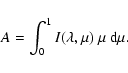
We can derive the monochromatic visibility law
![]() from the monochromatic intensity profile
from the monochromatic intensity profile
![]() using the Hankel integral:
using the Hankel integral:
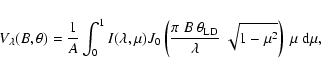 |
(1) |
 |
(2) |
![\begin{displaymath}V_K(B,\theta) = \frac{\int_K{ \left[V_\lambda(B, \theta)\
T(\...
...lambda)\ S(\lambda)\right]^2~\lambda^2 ~{\rm d}\lambda }}\cdot
\end{displaymath}](/articles/aa/full/2006/05/aa3187-05/img72.gif) |
(3) |
This formulation is very general, as it does not make any particular
assumption about the spectrum of the star or about the wavelength
dependence of its intensity profile
![]() .
.
Considering the model discussed in Sect. 4.1, we now
derive the limb-darkened angular diameter
![]() of
of
![]() Cen B. It is obtained by a standard
Cen B. It is obtained by a standard ![]() analysis of the data. We define the reduced
analysis of the data. We define the reduced ![]() of our fit by
of our fit by
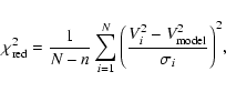 |
(4) |
The ![]() minimization was computed for three center-to-limb
models: uniform disk (UD), 1D ATLAS, and 3D RHD. In each case, the
broadband square visibility curve
minimization was computed for three center-to-limb
models: uniform disk (UD), 1D ATLAS, and 3D RHD. In each case, the
broadband square visibility curve
![]() is shown in
Figs. 4 and 5. In addition to the
purely statistical error, we must also take two systematic error
sources into account: the calibration uncertainty and the wavelength
uncertainty. The calibration uncertainty comes from the errors on
the a priori angular sizes of the five calibrators that were
used for the VINCI observations. It amounts to 0.012 mas on the
final angular diameter. The wavelength uncertainty comes from the
imperfect knowledge of the transmission of VINCI, in particular of
its fluoride glass optical fibers. This transmission was calibrated
on the sky (Paper I), and the uncertainty on this measurement is
estimated to be 0.15%. As it impacts linearly on the angular
diameter value, it corresponds to 0.009 mas. These two systematic
factors add up quadratically to the 0.013 mas statistical
uncertainty and result in a total error of 0.021 mas on the angular
diameters of
is shown in
Figs. 4 and 5. In addition to the
purely statistical error, we must also take two systematic error
sources into account: the calibration uncertainty and the wavelength
uncertainty. The calibration uncertainty comes from the errors on
the a priori angular sizes of the five calibrators that were
used for the VINCI observations. It amounts to 0.012 mas on the
final angular diameter. The wavelength uncertainty comes from the
imperfect knowledge of the transmission of VINCI, in particular of
its fluoride glass optical fibers. This transmission was calibrated
on the sky (Paper I), and the uncertainty on this measurement is
estimated to be 0.15%. As it impacts linearly on the angular
diameter value, it corresponds to 0.009 mas. These two systematic
factors add up quadratically to the 0.013 mas statistical
uncertainty and result in a total error of 0.021 mas on the angular
diameters of ![]() Cen B.
The best fit angular diameter that we derive using our 3D
limb-darkening model is
Cen B.
The best fit angular diameter that we derive using our 3D
limb-darkening model is
![]() mas. The 1D
model produces a slightly larger diameter,
mas. The 1D
model produces a slightly larger diameter,
![]() mas, and the UD disk produces naturally a much smaller
diameter,
mas, and the UD disk produces naturally a much smaller
diameter,
![]() mas.
mas.
There is no significant difference between the three models in the first lobe of visibility. However, different amplitudes of the second lobe were observed. While the UD model produces higher visibilities, the 1D limb-darkened model leads to visibilities that are slightly too low compared to our observations. Overall, the 3D model leads to a slightly better agreement with observations.
As expected, the difference 3D/1D is rather small, since we are
working in the near-infrared (K-band) and with a dwarf star. It is
nonetheless comparable to
![]() and therefore
significant.
and therefore
significant.
![\begin{figure}
\par\includegraphics[width=8cm,clip]{3187fig5.ps}\end{figure}](/articles/aa/full/2006/05/aa3187-05/img83.gif) |
Figure 4:
Overview of |
| Open with DEXTER | |
![\begin{figure}
\par\includegraphics[width=8cm,clip]{3187fig6.ps}\hspace*{7mm}
\includegraphics[width=8.2cm,clip]{3187fig7.ps}\end{figure}](/articles/aa/full/2006/05/aa3187-05/img84.gif) |
Figure 5:
Close-up views of
the squared visibilities of |
| Open with DEXTER | |
Assuming the parallax value of Söderhjelm (1999),
![]() mas
mas![]() , we found a linear radius of
, we found a linear radius of
![]() which agrees with results presented in Paper 1.
We estimated that the adopted uncertainty in
which agrees with results presented in Paper 1.
We estimated that the adopted uncertainty in
![]() (=50 K) leads to an error of about
(=50 K) leads to an error of about
![]() ,
i.e. ten times
smaller than the derived uncertainties. From the 1D analysis, we
derived a radius of
,
i.e. ten times
smaller than the derived uncertainties. From the 1D analysis, we
derived a radius of
![]() ,
larger than the
radius found by the RHD approach by about
,
larger than the
radius found by the RHD approach by about
![]() .
In
addition to the corrections it provides, the use of 3D simulations
was also motivated by the absence of adjustable parameters, which is
not the case for 1D models.
.
In
addition to the corrections it provides, the use of 3D simulations
was also motivated by the absence of adjustable parameters, which is
not the case for 1D models.
This slightly smaller linear radius obtained from 3D RHD
simulations, compared with the one derived from 1D ATLAS model,
supports the suggestion of a smaller mass (
![]() ,
Kervella et al. 2003) rather than the larger one (
,
Kervella et al. 2003) rather than the larger one (
![]() )
proposed by Pourbaix et al. (2002). However,
stellar evolution models are sensitive to many parameters, and a
smaller radius does not always lead to a smaller mass. More
investigations are thus needed before we can reach a definite
conclusion about the mass of
)
proposed by Pourbaix et al. (2002). However,
stellar evolution models are sensitive to many parameters, and a
smaller radius does not always lead to a smaller mass. More
investigations are thus needed before we can reach a definite
conclusion about the mass of ![]() Cen B. In this context, our
improved radius provides an additional constraint on asteroseismic
diagnostics.
Cen B. In this context, our
improved radius provides an additional constraint on asteroseismic
diagnostics.
In this paper we improve determination of the radius of ![]() Cen B in two respects. Firstly, we report the first interferometric
measurements in the second lobe of visibility. Secondly, in order to
derive a reliable value of the angular diameter of the star, we
performed realistic 3D RHD simulations of the surface of
Cen B in two respects. Firstly, we report the first interferometric
measurements in the second lobe of visibility. Secondly, in order to
derive a reliable value of the angular diameter of the star, we
performed realistic 3D RHD simulations of the surface of ![]() Cen B. By comparison with observations, we found a radius of
Cen B. By comparison with observations, we found a radius of
![]() .
The correction provided by the 3D approach
is small but significant (especially in the K band probed with
VINCI), since it provides a radius that is smaller by roughly
.
The correction provided by the 3D approach
is small but significant (especially in the K band probed with
VINCI), since it provides a radius that is smaller by roughly
![]() compared with what can be obtained by 1D models.
Moreover, the use
of 3D RHD is preferable since it does not introduce adjustable
parameters to describe convection. We also emphasize
that for hotter A-F stars the correction due to 3D analysis will be
larger than for
compared with what can be obtained by 1D models.
Moreover, the use
of 3D RHD is preferable since it does not introduce adjustable
parameters to describe convection. We also emphasize
that for hotter A-F stars the correction due to 3D analysis will be
larger than for ![]() Cen B. We have shown that even for a
K-dwarf like
Cen B. We have shown that even for a
K-dwarf like ![]() Cen B, though it is small, the correction
obtained by the use of RHD simulations should not be neglected for
very high precision interferometric measurements. In the next few
years, the combination of high visibility precision and long
baselines will require the use of realistic theoretical models of
the stellar limb-darkening to extract the true photospheric angular
diameter of the observed stars from the observed visibilities.
Conversely, observations beyond the first minimum of the visibility
function will directly sample the light distribution on the surface
of the stars, therefore providing constraints for the atmosphere
structure models. Future observations with the VLTI will allow to
sample tightly the second lobe of the visibility function of several
solar analogs (including
Cen B, though it is small, the correction
obtained by the use of RHD simulations should not be neglected for
very high precision interferometric measurements. In the next few
years, the combination of high visibility precision and long
baselines will require the use of realistic theoretical models of
the stellar limb-darkening to extract the true photospheric angular
diameter of the observed stars from the observed visibilities.
Conversely, observations beyond the first minimum of the visibility
function will directly sample the light distribution on the surface
of the stars, therefore providing constraints for the atmosphere
structure models. Future observations with the VLTI will allow to
sample tightly the second lobe of the visibility function of several
solar analogs (including ![]() Cen A and B), and therefore to
derive their intensity profiles with high accuracy. Comparisons
between our theoretical predictions of limb-darkening and the future
observations made by AMBER will be an excellent test of our
modelling of the surface of
Cen A and B), and therefore to
derive their intensity profiles with high accuracy. Comparisons
between our theoretical predictions of limb-darkening and the future
observations made by AMBER will be an excellent test of our
modelling of the surface of ![]() Cen B. Indeed, AMBER will
provide new interferometric data that will contain much more
information compared with VINCI. There will be two major advantages
with AMBER:
Cen B. Indeed, AMBER will
provide new interferometric data that will contain much more
information compared with VINCI. There will be two major advantages
with AMBER:
Acknowledgements
We thank Vincent Coudé du Foresto for important remarks that led to improvements at an early stage of this paper. We thank the anonymous referee for constructive remarks. These interferometric measurements were obtained using the VLTI (ESO Paranal, Chile), and were retrieved from the ESO/ST-ECF Archive (Garching, Germany). LB thanks the CNES for financial support and Å. Nordlund for providing his RHD code. We also thank Claude Van't Veer for providing the ATLAS model.