A&A 446, 403-415 (2006)
DOI: 10.1051/0004-6361:20042540

The Hanle effect in a random medium

H. Frisch

Laboratoire Cassiopée (CNRS, UMR 6202), Observatoire de la Côte d'Azur, BP 4229, 06304 Nice Cedex 4, France

Received 15 December 2004 / Accepted 21 September 2005

Abstract
This paper considers the Hanle effect produced by a turbulent magnetic field. To overcome the simplified microturbulent treatment whereby the Hanle phase matrix is locally averaged over some magnetic field distribution, we consider a turbulent magnetic field with a finite correlation length. We assume that the magnetic field along each individual photon path can be represented by a Kubo-Anderson process (KAP) and study the stationary solution as time goes to infinity. A KAP is a discontinuous Markov process. The random magnetic field is characterized by a correlation length and a distribution function of the magnetic field vector; both can be chosen arbitrarily. The microturbulent limit is recovered when the correlation length goes to zero. A non-stochastic integral equation of the Wiener-Hopf type is obtained for a mean conditional source vector. This integral equation yields explicit expressions for the mean Stokes parameters, provided one makes physically realistic approximations, namely neglect the effect of the magnetic field on Stokes I, keep only the contributions from I and Q in the source terms for Stokes Q and Stokes U and solve the integral equation for Q with a two-scattering approximation. The final expressions involve mean values and correlation functions of some of the elements of the Hanle phase matrix and show the dependence on the correlation length of the random magnetic field.
The combined effects of a turbulent velocity field and a turbulent magnetic field with finite correlation lengths is also studied. The velocity field is represented by a KAP with the same correlation length as the magnetic field. Some of the velocity field effects are treated with an effective medium approximation as in Frisch & Frisch (1976, MNRAS, 175, 157). Explicit expressions are obtained for the mean Stokes parameters. They can account for correlations between velocity field and magnetic field fluctuations.

Key words: line: formation - polarization - magnetic fields - turbulence - radiative transfer

   
1 Introduction

The Hanle effect is a powerful diagnostic tool for the measurement of weak magnetic fields, deterministic or turbulent (Stenflo 1978; Sahal-Bréchot #Sahal-Br&; Stenflo 1982). Contrary to the Zeeman effect, the Hanle effect leaves a signature on the polarization even for an isotropically distributed random field with zero mean. The work of Stenflo and followers is based on the assumption that the magnetic field is microturbulent, namely that it has a correlation scale much smaller than a photon mean-free path around line center. One can then average the Hanle phase matrix over the distribution of the random magnetic field. If the latter is isotropically distributed, the Hanle problem reduces to a resonance polarization problem with a modified (smaller) polarization parameter (Stenflo 1982, 1994). All the determinations of solar turbulent magnetic fields have been carried out so far with this particular microturbulent magnetic field model (Faurobert-Scholl 1993, 1996; Faurobert et al. 2001; Trujillo Bueno at al. 2004; Bommier et al. 2005).

The diagnostic method is based on a comparison between the observed Stokes parameters and the Stokes parameters given by an atmospheric model with zero magnetic field. The magnetic field determination is therefore fairly sensitive to the atmospheric parameters and in particular to the assumed turbulent velocity field which influences the width and depth of the Stokes parameters profiles (Stenflo 1994). Nearly all determinations of the turbulent magnetic field in the quiet regions of the solar photosphere have been carried out with a turbulent velocity represented by a mixture of microturbulence and macroturbulence, each one being modeled by a Gaussian distribution. The micro and macroturbulent root mean square (rms) velocities are deduced from the frequency profiles of Stokes I, the microturbulent rms from the line width and the macroturbulent rms from the line center intensity. The sensitivity of the magnetic field determination to the choices of the micro and macro rms is discussed in Bommier et al. (2005). Recently Trujillo Bueno et al. (2004) have determined the mean magnetic field strength in the quiet sun, using a 3D hydrodynamical numerical simulation of the solar surface convection. The turbulent magnetic field is treated as usual with a microturbulent approximation.

To overcome the micro/macro turbulent approximation, we consider here the effects of random magnetic and velocity fields in which turbulent fluctuations have a wide range of wave numbers. This is actually the standard situation in stellar atmospheres because of the very large kinetic and magnetic Reynolds numbers. Our goal is to obtain mean values for the observable Stokes parameters. Our approach is largely inspired by the work carried out in the seventies on the broadening of spectral lines by a turbulent velocity with a finite correlation length. Several velocity field models with a finite correlation length were introduced to address this question. A detailed review can be found in Mihalas (1978). For the present investigation, we have chosen Kubo-Anderson processes (KAP) to model the random magnetic and velocity fields. We note here that Landi Degl'Innocenti (1994) (see also Landi Degl'Innocenti & Landolfi 2004, henceforth LL04) has used a KAP to study the Zeeman effect by a turbulent magnetic field.

A KAP is a step-wise stationary Markov process. It takes constant but random values on intervals of random length. It is characterized by a distribution function and a correlation length. The former gives the random values of the Markov process and the latter the mean distance between the jumps from one value to another. The Markov property is essential to obtain explicit expressions for mean quantities. A KAP has an exponential covariance. The microturbulent limit is recovered when the correlation length goes to zero and the macroturbulent limit when the correlation length goes to infinity.

The distribution of the magnetic field vector in the upper layers of the quiet photosphere is not well known nor are the correlations between magnetic field and velocity fields fluctuations. For isotropic turbulence, symmetry arguments give that these correlations are zero when the magnetic field is treated as a pseudo-vector (Domke & Pavlov 1979). In the usual magnetic field determinations based on a microturbulent description of the magnetic field associated with a micro/macro description of the velocity field, the magnetic field and velocity field fluctuations are fully decoupled. The method that we describe here shows how treat magnetic fields and velocity fields with a finite correlation length and can handle correlations between the magnetic field and velocity field fluctuations.

For spectral lines formed by multiple scatterings of photons, i.e. under non-LTE conditions, it is not possible, even with a Markov model, to obtain closed equations for mean quantities because the photons can return several time to the same turbulent element (Gail et al. 1975; Magnan 1975; Frisch & Frisch 1976, henceforth FF76). A way out of this difficulty is to assume a random process in time instead of a random process in space and then consider the stationary solution as time goes to infinity. This method was introduced in FF76 and worked out in Froeschlé & Frisch (#Froeschl&, henceforth FF80). The results of these papers are generalized here to treat the Hanle effect with random magnetic fields and velocity fields.

The outline of the paper is the following. In Sect. 2, we recall the transfer equation for the Hanle effect. In Sects. 3 to 5, we assume that the magnetic field only is random. In Sect. 3, we show how to set up the time-dependent transfer problem, introduce the random magnetic field model, construct a time-independent stochastic transfer equation and establish an integral equation for a mean conditional time-independent source vector. In Sect. 4 we explain how the problem can be simplified by taking into account some of the properties of the Hanle effect. In Sect. 5 we establish explicit expressions for the mean observable Stokes parameters. They involve the correlation length of the magnetic field and are constructed with a two-scattering approximation. Section 6 is devoted to the joint effects of turbulent magnetic and velocity fields.

	Figure 1: Reference system. Definition of $\theta$ and $\chi$, the inclination and longitude of the direction ${\mbox{\boldmath$\vec{\Omega}$ }}$.
Open with DEXTER

   
2 The transfer equation for the Hanle effect

We consider a plane parallel semi-infinite atmosphere and choose the reference system shown in Fig. 1 where z is the normal to the atmosphere. The Hanle effect, i.e., resonance scattering in the presence of a magnetic field, can be described by the three Stokes parameters I, Q, U. At any point in the medium the three-component Stokes vector ${\mbox{\boldmath$\vec{S}$ }}$ with components I, Q, U depends on z and on a direction ${\mbox{\boldmath$\vec{\Omega}$ }}$ defined by its two polar angles $\theta$ and $\chi$. It also depends on a frequency variable x. Here x is measured in Doppler width units with the zero at line center. We also assume a two-level atom with unpolarized ground level.

The full theory of the Hanle effect is still in a somewhat preliminary phase, in particular when it comes to describe the frequency redistribution at each scattering although some theoretical progress have been made by Bommier (1997a,b; see also Landi Degl'Innocenti et al. 1997). Observations are usually analyzed with some simplifying assumptions namely that the full redistribution matrix can be written as a sum of terms, each of which is the product of a frequency redistribution function r(x,x') by a scattering phase matrix $\hat R({\mbox{\boldmath$\vec{\Omega}$ }},{\mbox{\boldmath$\vec{\Omega}$ }'};{\mbox{\boldmath$\vec{H}$ }})$. Here ${\mbox{\boldmath$\vec{\Omega}$ }}$ and xare the direction and frequency of the incident beam, ${\mbox{\boldmath$\vec{\Omega}$ }'}$ and x' the direction and frequency of the scattered beam and ${\mbox{\boldmath$\vec{H}$ }}$ the magnetic field vector (see e.g. Domke & Hubeny 1998; Stenflo 1994, and references therein; Faurobert et al. 2001; Bommier et al. 2005; Holzreuter et al. 2005). For a two-level atom model, with unpolarized ground level and a redistribution function of the above type, each Stokes parameter can be written in the form

$$s_i(z,x,{\mbox{\boldmath$\vec{\Omega}$ }})=\sum_{KQ}{\mathcal T}^K_Q(i,{\mbox{\boldmath$\vec{\Omega}$ }})s^K_Q(z,x,\theta).$$ (1)

Here i=0,1,2 is the index of the Stokes component, with s₀=I, s₁=Q and s₂=U. The indices Kand Q take the values K=0,Q=0, $K=2,Q=\pm2,\pm1,0$. The ${\mathcal T}^K_Q$ are irreducible spherical tensors for polarimetry introduced by Landi Degl'Innocenti (1984) (see also LL04). The six functions s^K_Q depend on the inclination angle $\theta$ but not on the longitude $\chi$. They are complex quantities and, since the s_i are real, they satisfy the same conjugation property as the ${\mathcal T}^K_Q$, namely $(s^K_Q)^\ast=(-1)^Q s^K_{-Q}$, where $\ast$ stand for complex conjugate. Using the conjugation property, it is possible to construct six real functions : I₁=s⁰₀, I₂=s²₀, $I_3=2\Re(s^2_1)$, $I_4=2\Im(s^2_1)$; $I_5=2\Re(s^2_2)$, $I_6=2\Im(s^2_2)$. The Stokes parameters can then be written as

 

$${I={I}_1 + {1\over 2\sqrt2}(3\mu ^2 -1){ I}_2 }$$

$$~~~ -{\sqrt 3\over 2}\mu\sqrt{1-\mu ^2} ({I}_3 \cos \chi - {I}_4 \sin \chi)$$

$$~~~ + {\sqrt 3\over 4}(1-\mu ^2)({I}_5\cos2\chi - {I}_6\sin 2\chi),$$ (2)

 

$${Q=-{3\over 2\sqrt2}(1-\mu ^2){I}_2 }$$

$$~~~ -{\sqrt 3\over 2}\mu\sqrt{1-\mu ^2} ({I}_3 \cos \chi - {I}_4 \sin \chi)$$

$$~~~ - {\sqrt 3\over 4}(1+\mu ^2)({I}_5\cos 2\chi -{I}_6\sin 2\chi),$$ (3)

 

$$U={\sqrt 3\over 2}\sqrt{1-\mu ^2}({I}_3\sin \chi +{I}_4\cos \chi) + {\sqrt 3\over 2}\mu({I}_5\sin 2\chi + {I}_6\cos 2\chi).$$ (4)

A decomposition very similar to Eq. (1) was first given for the six real functions I_i by Faurobert-Scholl (1991) with a Fourier decomposition with respect to $\chi$ of the Stokes vector and of the Hanle phase matrix (see also Nagendra et al. 1998, henceforth NFF98; Frisch 1998, 1999, henceforth F99). Recently Loskutov (2004) and Ivanov (2004) have proposed a factorization of the phase matrix $\hat {R}$ which provides a simple method for achieving the same decomposition. Actually the simplest method to establish Eq. (1) is to write the phase matrices $\hat R({\mbox{\boldmath$\vec{\Omega}$ }},{\mbox{\boldmath$\vec{\Omega}$ }'};{\mbox{\boldmath$\vec{H}$ }})$ in terms of the irreducible tensors ${\mathcal T}^K_Q$, using expressions given in, e.g., LL04.

Here we make the assumption that the redistribution matrix contains a single term of the form $r(x,x')\hat R({\mbox{\boldmath$\vec{\Omega}$ }},{\mbox{\boldmath$\vec{\Omega}$ }'};{\mbox{\boldmath$\vec{H}$ }})$. For simplicity we also assume that there is no correlation between x and x', i.e. we assume complete frequency redistribution as in Landi Degl'Innocenti et al. (1990), for example. We then have $r(x,x')=\varphi(x)\varphi(x')$, where $\varphi(x)$ is the line absorption profile, normalized to unity. The I_i, can be used to form a six-component vector ${\mbox{\boldmath$\vec{I}$ }}(z,x,\theta)$. In the following we use this vector to represent the polarized field and refer to it as the irreducible Stokes vector.

The transfer equation for ${\mbox{\boldmath$\vec{I}$ }}$ can be written as

 

$$\mu {\partial {\mbox{\boldmath$\vec{I}$ }}\over \partial z}= -k(z... ...'){\mbox{\boldmath$\vec{I}$ }}(z,x',\mu')~{{\rm d}\mu'\over 2}~{\rm d}x'\Bigr].$$ (5)

Here $\mu=\cos\theta$. We have denoted k(z) the line frequency integrated absorption coefficient per unit length. The variables z and x have been introduced above. The vector ${\mbox{\boldmath$\vec{G}$ }}$ is a given source term. It is a six-component vector corresponding to a decomposition similar to Eq. (1) of a primary source term, often of thermal origin. If the latter is unpolarized, as assumed here, only the first component G₁ is non zero. $\hat M({\mbox{\boldmath$\vec{H}$ }})$ is a $6\times 6$ matrix which depends on the magnetic field and $\hat\Psi$ also a $6\times 6$matrix. The matrix $\hat{\cal E}$ accounts for inelastic collisions and elastic depolarizing collisions. It is a diagonal matrix. The $6\times 6$ unit matrix is simply denoted by 1. More details on these matrices are given in Sect. 4.

The Hanle effect acts only around the line center (Omont et al. 1973; LL04). In the line wings, the life-time of the upper level is too short for the magnetic field to destroy the phase coherences of the Zeeman sub-levels. A simple way to take this property into account is to consider that $\hat M$ becomes equal to the identity matrix for frequencies $\vert x\vert>x_{\rm c}$. Typically $x_{\rm c}\simeq 3$. The results are not very sensitive to the choice of $x_{\rm c}$. We explain on the final results how this cutoff can be implemented.

   
3 Time-dependent transfer problem

In the transfer equation, randomness comes through the matrix $\hat M$. Proceeding as in FF76, we assume that the magnetic field ${\mbox{\boldmath$\vec{H}$ }}$ is a function of time t, ${\mbox{\boldmath$\vec{H}$ }(t)}= {\mbox{\boldmath$\vec{H}$ }(z(t))}$, where z(t) is the random position of the photon at time t. Together with the time-dependent random magnetic field, we must use the time-dependent transfer equation,

 

$${1\over c}{\partial {\mbox{\boldmath$\vec{I}$ }}(t,z,x,\mu)\over ... ...si(\mu') {\mbox{\boldmath$\vec{I}$ }}(t,z,x',\mu')~{\rm d}\mu'~{\rm d}x'\Bigg],$$ (6)

where c is the velocity of light. We have used the compact notation

$$\int_{x\mu}{\rm d}\mu~{\rm d}x =\int_{-\infty}^{+\infty}\int_{-1}^{+1}{{\rm d}\mu\over 2}~{\rm d}x.$$ (7)

In addition, we must prescribe an initial condition ${\mbox{\boldmath$\vec{I}$ }}^{(0)}= {\mbox{\boldmath$\vec{I}$ }}(0,z,x,\mu)$. We assume that the primary source ${\mbox{\boldmath$\vec{G}$ }}$ is time-independent. Hence, Eq. (6) has a stationary solution. We are interested in the mean value of this solution.

   
3.1 The magnetic field model

As mentioned in Sect. 1, we assume that the random magnetic field can be represented by a KAP. A KAP is a step-wise constant Markov process which jumps at randomly chosen points between random step-values. The jumping points t_i are uniformly and independently distributed in $[-\infty,+\infty]$ with a Poisson distribution of density $1/t_{\rm corr}$. In each interval t_i-1< t < t_i, the magnetic field takes a constant value ${\mbox{\boldmath$\vec{H}$ }}(t)= {\mbox{\boldmath$\vec{H}$ }}_i$. The ${\mbox{\boldmath$\vec{H}$ }}_i$ are random variables with a probability density $P({\mbox{\boldmath$\vec{H}$ }})$. A KAP is therefore characterized by a correlation time $t_{\rm corr}$ and a probability density $P({\mbox{\boldmath$\vec{H}$ }})$.

This type of process was introduced in connection with nuclear magnetic resonance (Anderson 1954; Kubo 1954). It was used to model the stochastic Stark effect (Frisch & Brissaud 1971; Brissaud & Frisch 1971). For radiative transfer, it was employed to study the broadening of spectral lines by a turbulent velocity field (Auvergne et al. 1973). The denomination KAP was introduced in this context. The KAP, and some generalized versions, are discussed in detail in Brissaud & Frisch (1974), a review article on the solution of linear stochastic differential equations.

As ${\mbox{\boldmath$\vec{H}$ }}$ is a stationary Markov random process (Wang & Uhlenbeck 1945; Barucha-Reid 1960; Papoulis 1965; Feller 1971), the transition probability density $P_{\rm tr}({\mbox{\boldmath$\vec{H}$ }},t\vert{\mbox{\boldmath$\vec{H}$ }'})$, such that $P_{\rm tr}~{\rm d}^3{\mbox{\boldmath$\vec{H}$ }}$ is the probability to find a field ${\mbox{\boldmath$\vec{H}$ }}$ (within ${\rm d}^3{\mbox{\boldmath$\vec{H}$ }}$) at time s+t, given a field ${\mbox{\boldmath$\vec{H}$ }'}$ at time s, satisfies the Kolmogorov equation

$${\partial P_{\rm tr}({\mbox{\boldmath$\vec{H}$ }},t\vert{\mbo... ...oldmath$\vec{H}$ }'})~{\rm d}^3{\mbox{\boldmath$\vec{H}$ }''}.$$ (8)

Here $\Pi$ is an integral operator which defines the Markov process. For diffusion processes, like the Brownian motion or the Ornstein-Uhlenbeck process (Uhlenbeck & Ornstein 1930; Feller 1971), the Kolmogorov equation is actually a second-order differential equation. In the modern terminology, it is called a Fokker-Planck equation. The stationary solution of the Kolmogorov equation is the distribution $P({\mbox{\boldmath$\vec{H}$ }})$. The transition probability satisfies

$$\int P_{\rm tr}({\mbox{\boldmath$\vec{H}$ }''},t\vert{\mbox{\boldmath$\vec{H}$ }'})~{\rm d}^3{\mbox{\boldmath$\vec{H}$ }''}=1,$$ (9)

with the initial condition

$$P_{\rm tr}({\mbox{\boldmath$\vec{H}$ }},0\vert{\mbox{\boldmat... ...a({\mbox{\boldmath$\vec{H}$ }}-{\mbox{\boldmath$\vec{H}$ }'}),$$ (10)

where $\delta$ is the Dirac distribution. For a KAP,

$$\Pi({\mbox{\boldmath$\vec{H}$ }},{\mbox{\boldmath$\vec{H}$ }'... ...ldmath$\vec{H}$ }'}) - P({\mbox{\boldmath$\vec{H}$ }})\right].$$ (11)

The solution of the Kolmogorov equation is

$$P_{\rm tr}({\mbox{\boldmath$\vec{H}$ }},t\vert{\mbox{\boldmat... ... (1-{\rm e}^{-t/t_{\rm corr}})P({\mbox{\boldmath$\vec{H}$ }}).$$ (12)

The first term gives the probability that the magnetic field keeps its initial value ${\mbox{\boldmath$\vec{H}$ }'}$ after an interval of time t and the second term the probability that it takes a value ${\mbox{\boldmath$\vec{H}$ }}$, with probability $P({\mbox{\boldmath$\vec{H}$ }})$.

   
3.2 The mean conditional irreducible Stokes vector

Equation (6) is a stochastic differential equation with Markov coefficients to which we can apply the standard technique of solution (Frisch 1968). Symbolically, Eq. (6) can be written as

$${1\over c}{\partial {\mbox{\boldmath$\vec{I}$ }}\over\partial... ...oldmath$\vec{I}$ }}(t) + {\cal A}{\mbox{\boldmath$\vec{G}$ }},$$ (13)

where ${\cal L}$ is a linear operator which depends deterministically on the Markov process ${\mbox{\boldmath$\vec{H}$ }}(t)$ and ${\cal A}=k(z)\varphi(x)$. The crucial remark is that the joint process $\{{\mbox{\boldmath$\vec{H}$ }}(t),{\mbox{\boldmath$\vec{I}$ }}(t)\}$ is also a Markov process. Its probability density ${\cal P}({\mbox{\boldmath$\vec{H}$ }},{\mbox{\boldmath$\vec{I}$ }};t)$ satisfies

$${\partial {\cal P}\over\partial t}= \Pi{\cal P} -c \sum_{l=1}... ...}}){\mbox{\boldmath$\vec{I}$ }} + {\cal A}G_l] {\cal P}\Bigr].$$ (14)

The index l refers to the 6 components of ${\mbox{\boldmath$\vec{I}$ }}$. The first term expresses the change between t and $t + {\rm d}t$ of the probability density of the magnetic field and the following terms the change in the probability of the components of ${\mbox{\boldmath$\vec{I}$ }}$ which evolve according to Eq. (13). The initial condition is

$${\cal P}({\mbox{\boldmath$\vec{H}$ }},{\mbox{\boldmath$\vec{I... ...ath$\vec{H}$ }})\prod_{l=1}^6\delta\left(I_l-I_l^{(0)}\right).$$ (15)

We now introduce a mean conditional irreducible Stokes vector ${\mbox{\boldmath$\vec{\cal I}$ }}(t,z,x,\mu\vert{\mbox{\boldmath$\vec{H}$ }})$. Each component ${\cal I}_k$ is defined for k=1 to 6 by

$${\cal I}_k(t,z,x,\mu\vert{\mbox{\boldmath$\vec{H}$ }})= {1\ov... ...\mbox{\boldmath$\vec{I}$ }};t)I_k~{\rm d}I_1\ldots~{\rm d}I_6.$$ (16)

We stress that ${\mbox{\boldmath$\vec{\cal I}$ }}$ is a conditional mean. Indeed, ${\cal P}({\mbox{\boldmath$\vec{H}$ }},{\mbox{\boldmath$\vec{I}$ }};t)/P({\mbox{\boldmath$\vec{H}$ }})$ is the conditional probability density of ${\mbox{\boldmath$\vec{I}$ }}$ at time t, knowing ${\mbox{\boldmath$\vec{H}$ }}(t)= {\mbox{\boldmath$\vec{H}$ }}$. To obtain the mean irreducible Stokes vector itself, it suffices to average ${\mbox{\boldmath$\vec{\cal I}$ }}$ over ${\mbox{\boldmath$\vec{H}$ }}$ with the density $P({\mbox{\boldmath$\vec{H}$ }})$. Here conditional means are denoted with calligraphic uppercase letters and means over the magnetic distribution with Roman letters.

Equation (14), is the starting point to construct a closed transfer equation for each ${\cal I}_k$ : it suffices to multiply it by I_k and then to integrate as in Eq. (16). The terms involving the partial derivatives in the r.h.s. of Eq. (14) can be integrated by parts. The integrated term is zero because of the factor ${\cal P}$. The remaining integral contains only the term corresponding to l=k. One thus obtains

$${1\over c}{\partial {\cal I}_k\over\partial t} = {1\over c}\P... ...h$\vec{H}$ }}){\mbox{\boldmath$\vec{\cal I}$ }} + {\cal A}G_k,$$ (17)

where

$$\Pi_1 ={1\over P({\mbox{\boldmath$\vec{H}$ }})}\Pi({\mbox{\bo... ...\mbox{\boldmath$\vec{H}$ }'})P({\mbox{\boldmath$\vec{H}$ }'}).$$ (18)

${\cal L}_k$ is the k-component of the operator ${\cal L}$. We can write this result in the vectorial form

$${1\over c}{\partial {\mbox{\boldmath$\vec{\cal I}$ }}\over\pa... ...c{G}$ }} + {1\over c}\Pi_1 {\mbox{\boldmath$\vec{\cal I}$ }},$$ (19)

where ${\cal L}$ is the transfer operator. In explicit notation, Eq. (19) can be written as

 

$${{1\over c}{\partial {\mbox{\boldmath$\vec{\cal I}$ }}(t,z,x,\mu\... ...vec{\cal I}$ }}(t,z,x,\mu\vert{\mbox{\boldmath$\vec{H}$ }})\over \partial z} =}$$

$$\qquad -k(z)\varphi(x){\mbox{\boldmath$\vec{\cal I}$ }}(t,z,x,\mu... ...ox{\boldmath$\vec{H}$ }}) + k(z)\varphi(x)\Bigl[{\mbox{\boldmath$\vec{G}$ }}(z)$$

$$\qquad +(1-\hat{\cal E})\hat M({\mbox{\boldmath$\vec{H}$ }})\int_... ...}$ }}(t,z,x',\mu'\vert{\mbox{\boldmath$\vec{H}$ }})~{\rm d}\mu'~{\rm d}x'\Bigr]$$

$$\qquad + {1\over c}\int \Pi_1({\mbox{\boldmath$\vec{H}$ }},{\mbox... ...\mu\vert{\mbox{\boldmath$\vec{H}$ }'}) ~{\rm d}^3{\mbox{\boldmath$\vec{H}$ }'}.$$ (20)

There is an initial condition

$${\mbox{\boldmath$\vec{\cal I}$ }}(0,z,x,\mu\vert{\mbox{\boldm... ...dmath$\vec{I}$ }}^{(0)}(z,x,\mu,{\mbox{\boldmath$\vec{H}$ }}).$$ (21)

   
3.3 Stationary transfer equation for the mean conditional irreducible Stokes vector ${\mbox{\boldmath$\vec{\cal I}$ }}$

We are interested in the stationary solution only, so we set $\partial/\partial t=0$. This solution is independent of the initial condition ${\mbox{\boldmath$\vec{I}$ }}^{(0)}$. We introduce the line optical depth defined as ${\rm d}\tau = - k(z)~{\rm d}z$. We thus obtain for ${\mbox{\boldmath$\vec{\cal I}$ }}$ the transfer equation

 

$$\mu {\partial {\mbox{\boldmath$\vec{\cal I}$ }}(\tau,x,\mu\vert{\... ...\mu \vert{\mbox{\boldmath$\vec{H}$ }'})~{\rm d}^3{\mbox{\boldmath$\vec{H}$ }'},$$ (22)

where

 

$${\mbox{\boldmath$\vec{\cal S}$ }}(\tau\vert{\mbox{\boldmath$\vec{... ...c{\cal I}$ }}(\tau,x,\mu\vert{\mbox{\boldmath$\vec{H}$ }})~{\rm d}\mu~{\rm d}x.$$ (23)

In the following we refer to ${\mbox{\boldmath$\vec{\cal S}$ }}(\tau\vert{\mbox{\boldmath$\vec{H}$ }})$as the mean conditional source vector. The boundary conditions are given at the surface $\tau=0$ and at infinity. We assume as usual that the radiation incident on the surface is zero and that it tends to ${\mbox{\boldmath$\vec{G}$ }}(\tau)$ at infinity. In addition, boundedness for $\vert{\mbox{\boldmath$\vec{H}$ }}\vert\to \infty$ must be assumed to ensure uniqueness of the solution of Eq. (22).

The operator $\Pi$ introduced in Eq. (11) contains a correlation time scale $t_{\rm corr}$. The corresponding spatial correlation scale measured in optical depth units is $\tau_{\rm corr}(\tau)=c k(\tau)t_{\rm corr}$. It is convenient to introduce $\nu=1/\tau_{\rm corr}$ which can be interpreted as a mean number of turbulent eddies per unit optical depth. Here we assume that $\nu$ is independent of optical depth. To simplify the notation, we redefine the operator $\Pi_1$ such that

$${1\over c k(\tau)}\Pi_1 \longrightarrow \nu\Pi_1,$$ (24)

with the new $\Pi_1$ defined by

$$\Pi_1= - {1\over P({\mbox{\boldmath$\vec{H}$ }})}\left[\delta... ...\boldmath$\vec{H}$ }})\right]P({\mbox{\boldmath$\vec{H}$ }'}).$$ (25)

We observe here for future use that

$$-\Pi_1 f = f({\mbox{\boldmath$\vec{H}$ }}) - \langle f({\mbox{\boldmath$\vec{H}$ }})\rangle; \quad \langle\Pi_1 f\rangle=0,$$ (26)

for any function $f({\mbox{\boldmath$\vec{H}$ }})$. To obtain this result, we multiply Eq. (25) by $f({\mbox{\boldmath$\vec{H}$ }'})$ and integrate over ${\mbox{\boldmath$\vec{H}$ }'}$. We note also that

$$\Pi_1\langle f\rangle= 0; \quad \mbox{hence}\quad \Pi_1^n= \Pi_1,$$ (27)

for all powers n of $\Pi_1$.

   
3.4 Integral equation for the mean conditional source vector ${\mbox{\boldmath$\vec{\cal S}$ }}$

From the equation of transfer for ${\mbox{\boldmath$\vec{\cal I}$ }}(\tau,x,\mu\vert{\mbox{\boldmath$\vec{H}$ }})$, we can construct an integral operator equation for ${\mbox{\boldmath$\vec{\cal S}$ }}(\tau\vert{\mbox{\boldmath$\vec{H}$ }})$ by the usual method. Writing the operator $\Pi_1$ as an abstract operator, the formal solution of Eq. (22) can be written as

 

$${\mbox{\boldmath$\vec{\cal I}$ }}(\tau,x,\mu\vert{\mbox{\boldmath... ...ox{\boldmath$\vec{\cal S}$ }}(\tau'\vert~\cdot)~ {{\rm d}\tau'\over\mu};~\mu>0;$$ (28)

 

$${\mbox{\boldmath$\vec{\cal I}$ }}(\tau,x,\mu\vert{\mbox{\boldmath... ...ox{\boldmath$\vec{\cal S}$ }}(\tau'\vert~\cdot)~ {{\rm d}\tau'\over\mu};~\mu<0.$$ (29)

The source vector ${\mbox{\boldmath$\vec{\cal S}$ }}$ is a function of the magnetic field, but its dependence cannot be written explicitly because of the exponential operator. The magnetic field dependence is indicated by a dot. Here $\varphi$ stands for $\varphi(x)$ times the operator unity. Inserting this formal solution into Eq. (23), we obtain an operator integral equation of the Wiener-Hopf type,

 

$${\mbox{\boldmath$\vec{\cal S}$ }}(\tau\vert{\mbox{\boldmath$\vec{... ...h$\vec{H}$ }}){\mbox{\boldmath$\vec{\cal S}$ }}(\tau'\vert~\cdot)~{\rm d}\tau',$$ (30)

where the operator ${\cal K}$ is defined by

 

$${\cal K}(\tau;{\mbox{\boldmath$\vec{H}$ }}) = \int_{x\mu}^{\rm wh... ...ert\tau\vert\over \mu}(\varphi - \nu\Pi_1)\Bigr]\varphi(x)~{\rm d}\mu~{\rm d}x.$$ (31)

We have introduced the notation

$$\int_{x\mu}^{\rm wh}~{\rm d}\mu~{\rm d}x= \int_{-\infty}^{+\infty}\int_0^{1}{1\over 2\mu}~{\rm d}\mu~{\rm d}x.$$ (32)

Equations (22) and (30) have the structure of ordinary vectorial transfer equations, but with an additional independent 3D variable ${\mbox{\boldmath$\vec{H}$ }}$. Attempts to solve these equations numerically will encounter serious difficulties. The problem can be simplified by taking advantage of some properties of the Hanle effect.

   
4 A simplified Hanle problem

Polarization produced by resonance scattering is always weak since it is created by the anisotropy of the radiation field. In the presence of a magnetic field, the polarization becomes in general even weaker. Approximations based on this remark have been shown to give very satisfactory results with errors falling within the error bar of standard measurements (Faurobert-Scholl 1991; NFF98). They will allow us to obtain an explicit expression for the mean observable Stokes parameters. Before we describe the approximation, we must recall the meaning of the three matrices in Eq. (5) (see also Eq. (23)).

The matrices $\hat M$, $\hat\Psi$ and $\hat{\cal E}$ are $6\times 6$matrices with lines and columns numbered from 1 to 6. The elements of these matrices can be found in Faurobert-Scholl (1991) (see also NFF98; F99). Here we give only a few of them. We note also that signs may be different from those of the above mentioned articles because of sign differences in the elements of the vector ${\mbox{\boldmath$\vec{\cal I}$ }}$. The first line and first column of $\hat M$ contain only zeros, except for M_1,1=1 (we drop the symbol hat when we refer to elements of these matrices). The others 25 elements of $\hat M$ are non zero and depend on the magnetic field (strength and direction). In $\hat\Psi$, only the diagonal elements and the two off diagonal elements $\Psi_{1,2}= \Psi_{2,1}$ are non zero. The non zero elements are $\Psi_{1,1}=1$,

 

$$\Psi_{1,2}(\mu) {{\sqrt W_2}\over2\sqrt 2}(3\mu^2-1),$$ =

$$\Psi_{2,2}(\mu) {W_2\over 4}(5-12\mu^2 + 9\mu^4).$$ = (33)

The other non-zero elements, $\Psi_{3,3}=\Psi_{4,4}$ and $\Psi_{5,5}=\Psi_{6,6}$ are not used here. Henceforth we assume W₂=1, value corresponding to a normal Zeeman triplet. The matrix $\hat{\cal E}$ is diagonal with ${\cal E}_{1,1}=\epsilon_o$ and ${\cal E}_{k,k}=\epsilon_p$ for k=2 to 6. The parameter $\epsilon_o$ describes destruction by inelastic collisions and $\epsilon_p$ depolarization by elastic collisions. One roughly has $\epsilon_o\simeq \Gamma_{\rm I}/\Gamma_{\rm R}$ and $\epsilon_p\simeq D^{(2)}/\Gamma_{\rm R}$ where $\Gamma_{\rm I}$ is the inelastic collision rate, $\Gamma_{\rm R}$ the radiative de-excitation rate and D⁽²⁾ the collisional depolarization rate. If $D^{(2)}\ll \Gamma_{\rm I}$ then $\epsilon_p\simeq \epsilon_o$ (for the full definitions of $\epsilon_o$ and $\epsilon_p$, see Frisch 1998; also Faurobert et al. 2001; Bommier et al. 2005; LL04 Sect. 5.14).

In Eq. (5), the source term (inside the square bracket) can be written as ${\mbox{\boldmath$\vec{S}$ }}(z)={\mbox{\boldmath$\vec{G}$ }}(z) + (1-\hat{\cal E})\hat M({\mbox{\boldmath$\vec{H}$ }}){\mbox{\boldmath$\vec{J}$ }}(z)$, where ${\mbox{\boldmath$\vec{J}$ }}(z)$ is a 6-component vector. Numerical solutions of Eq. (5) (see NFF98) show that J₂ is roughly ten times smaller than J₁ and that the other J_k with $k=3,\ldots,6$ are roughly ten times smaller than J₂. To evaluate the source function, it is actually sufficient to keep the two first columns in the matrix $\hat M$ and set all the other elements to zero (in the first column, only the element M_1,1 is not zero). With this approximation we keep in the source terms the contributions from the Q=0 components, s⁰₀=I₁ and s²₀=I₂, only. The transfer equations for the I_k take thus much simpler forms.

The transfer equation for I₁ becomes the usual scalar one,

 

$$\mu{\partial I_1(\tau,x,\mu)\over \partial\tau} = \varphi(x) I_1(... ...o)\int_{x'\mu'} \varphi(x')I_1(\tau,x',\mu')~{\rm d}\mu'~{\rm d}x' + G_1\Bigr].$$ (34)

It contains no random elements, hence I₁ is not random.

The transfer equation for I₂ is

$$\mu{\partial I_2(\tau,x,\mu)\over \partial\tau} = \varphi(x) \bigl[I_2(\tau,x,\mu) - S_2(\tau)\bigr],$$ (35)

where

 

$$S_2(\tau)= (1-\epsilon_p)M_{2,2}({\mbox{\boldmath$\vec{H}$ }}) \l... ...int_{x\mu}\Psi_{2,2}(\mu)\varphi(x) I_2(\tau,x,\mu)~{\rm d}\mu~{\rm d}x\right],$$ (36)

with

$$C_{\rm I}(\tau) = \int_{x\mu} \varphi(x)\Psi_{1,2}(\mu)I_1(\tau,x,\mu)~{\rm d}\mu~{\rm d}x.$$ (37)

The definition of $\int_{x\mu}$ is given in Eq. (32). Since I₁ is non random, $C_{\rm I}$ is non random either. It plays the role of a primary source term for the Stokes parameter Q. Actually $C_{\rm I}$ is the dominant term in the component $\bar J^2_0$ of the frequency averaged irreducible tensor of the radiation field $\bar J^K_Q$(LL04). When the radiation field is isotropic, $C_{\rm I}$ is zero. In the equation for I₂, randomness comes thus from the matrix element M_2,2. Since this equation contains a scattering term involving I₂, it presents the same kind of difficulties as Eq. (5), but it is possible, in contrast with Eq. (5), to make physically reasonable assumptions which permit the calculation of the mean value of I₂, as shown below.

The transfer equations for I_k, $k=3,\ldots,6$, are of the form

$$\mu{\partial I_k(\tau,x,\mu)\over \partial\tau} = \varphi(x) \bigl[I_k(\tau,x,\mu) - S_k(\tau)\bigr],$$ (38)

with $S_k(\tau)$ given by Eq. (36) where M₂₂ should be replaced by M_k2, while the two terms in the square bracket are unchanged. Thus, the equations for the I_k have no scattering terms. Randomness comes from the matrix elements M_k,2 and from I₂. The solution of the transfer problem for I₂ will allow us to calculate the mean values of the I_k for k=3 to 6.

   
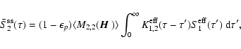
5 Mean Stokes Q and U

We show in this Section how to determine the mean values of I_k, $k=2,\ldots,6$. Equations (2) to (4) will then give us the mean values of the Stokes parameters Q and U and the magnetic field dependent terms in the expansion of Stokes I.

We introduce ${\cal I}_2$, the conditional mean of I₂ and apply the technique described in Sect. 3 to Eq. (35). In Sect. 5.1, we construct an integral equation similar to Eq. (30) for a mean conditional source function ${\cal S}_2(\tau\vert{\mbox{\boldmath$\vec{H}$ }})$. A Neumann series expansion of this integral equation, limited to the two first terms, yields an explicit expression for ${\cal S}_2(\tau\vert{\mbox{\boldmath$\vec{H}$ }})$as is shown in Sect. 5.2. In Sect. 5.3, we show how to average ${\cal S}_2(\tau\vert{\mbox{\boldmath$\vec{H}$ }})$ over the magnetic field distribution. We thus obtain a mean source function $\bar S_2(\tau)$ which is used in Sect. 5.4 to calculate the mean value of ${\cal I}_2$. In Sect. 5.5, we show how to construct the mean values of the ${\cal S}_k(\tau\vert{\mbox{\boldmath$\vec{H}$ }})$ and ${\cal I}_k$, for $k=3,\ldots,6$.

   
5.1 Stokes Q. Integral equation for the mean conditional source function ${\cal S}_{2}$

Following the procedure described in Sect. 3, we deduce from Eqs. (22) and (23) the transfer equation,

 

$$\mu {\partial {\cal I}_2(\tau,x,\mu\vert{\mbox{\boldmath$\vec{H}$... ...\mu \vert{\mbox{\boldmath$\vec{H}$ }'})~{\rm d}^3{\mbox{\boldmath$\vec{H}$ }'},$$ (39)

where

 

$${\cal S}_2(\tau\vert{\mbox{\boldmath$\vec{H}$ }})= (1-\epsilon_p)... ...al I}_2(\tau,x,\mu\vert{\mbox{\boldmath$\vec{H}$ }})~{\rm d}\mu~{\rm d}x\Bigg].$$ (40)

Inserting the formal solution of Eq. (39) into Eq. (40), we obtain for ${\cal S}_{2}$ the Wiener-Hopf integral equation

 

$${\cal S}_2(\tau\vert{\mbox{\boldmath$\vec{H}$ }})= (1-\epsilon_p)... ...\mbox{\boldmath$\vec{H}$ }}) {\cal S}_2(\tau'\vert~\cdot)~{\rm d}\tau' \right],$$ (41)

where the operator ${\cal K}_{2,2}$ is given by

 

$${\cal K}_{2,2}(\tau;{\mbox{\boldmath$\vec{H}$ }}) = \int_{x\mu}^{... ...\Bigl[-{\vert\tau\vert\over \mu}(\varphi - \nu\Pi_1)\Bigr]~{\rm d}\mu~{\rm d}x.$$ (42)

As pointed out, solving this integral equation where ${\mbox{\boldmath$\vec{H}$ }}$ is an independent variable will be a very laborious task. We now construct an approximate solution by way of a Neumann series expansion.

   
5.2 Neumann series expansion

The Neumann series expansion method of solution applies to any type of integral equations. For simplicity, we present it for the integral equation satisfied by $S_2(\tau)$ and then apply it to Eq. (41).

The formal solution of Eq. (35) yields the integral equation

 

$$S_2(\tau)= (1-\epsilon_p)M_{2,2}({\mbox{\boldmath$\vec{H}$ }}) \l... ...rm I}(\tau) + \int_0^\infty K_{2,2}(\tau-\tau') S_2(\tau')~{\rm d}\tau'\right],$$ (43)

where

$$K_{2,2}(\tau)=\int_{x\mu}^{\rm wh}\varphi ^2(x)\Psi_{2,2}(\mu... ...{\vert\tau\vert\varphi(x)\over\mu}\right]~{\rm d}\mu~{\rm d}x.$$ (44)

Here ${\mbox{\boldmath$\vec{H}$ }}$ is any magnetic field, random or not. For the component I₁, one can also introduced a source function S₁ defined as S₂ with $\epsilon_p$replaced by $\epsilon_o$, M_2,2 replaced by M_1,1, $\Psi_{2,2}$by $\Psi_{1,1}$ and the primary source term $C_{\rm I}(\tau)$ replaced by $G_1(\tau)$. The source function S₁ satisfies an integral equation similar to Eq. (43). Although the equations for S₁ and S₂ look formally the same, they have quite different behaviors because the integral of $\Psi_{1,1}$ over $\mu$ is equal to unity while the integral of $\Psi_{2,2}$ is equal to 7/10 as can be easily deduced from Eq. (33). Therefore the integral of K_2,2 over $\tau$(from $-\infty$ to $+\infty$) is also equal to 7/10 (we recall that $\varphi(x)$ is normalized to unity). To construct the solution of Eq. (43), it is convenient to introduce a renormalized kernel $K_{2,2}^\ast=(10/7)K_{2,2}$, normalized to unity, and an albedo for single scattering $\lambda_2={7\over 10}(1-\epsilon_p)M_{2,2}$. The Neumann series expansion for S₂ can thus be written

 

$${S_2(\tau)= (1-\epsilon_p)M_{2,2}({\mbox{\boldmath$\vec{H}$ }})C_{\rm I}(\tau) }$$

$$\qquad+\sum_{n=1}^{\infty} \lambda_2^n\int_0^\infty {\rm d}\tau_1... ...\ast(\tau-\tau_1)\int_0^\infty {\rm d}\tau_2~ K_{2,2}^\ast(\tau_1-\tau_2)\ldots$$

$$\qquad\int_0^\infty {\rm d}\tau_n ~K_{2,2}^\ast(\tau_{n-1}-\tau_{n})C_{\rm I}(\tau_{n}).$$ (45)

The term of order n gives the contribution of all the photons that have been scattered n times after creation by the primary source term. Its magnitude is order of $\lambda_2^n$ since $K_{2,2}^\ast$ is normalized to unity. It is easy to see that $\lambda_2$ is smaller than unity. Even if $(1-\epsilon_p)$ is close to unity, the two other factors are significantly smaller than unity (M_2,2 is equal to one only if the magnetic field is zero). Hence a few terms should suffice to properly represent the solution of the integral Eq. (43). We remark also that the accuracy of a truncated Neumann series expansion is not directly related to the optical depth of the line. The latter affects mainly the optical depth dependence of $C_{\rm I}$. It is clear that a Neumann series expansion would not be a good method to calculate I₁, i.e. Stokes I, since $\lambda_1=1-\epsilon_o$ is extremely close to unity. Spectral lines that are used to evaluate the solar turbulent magnetic field with the Hanle effect typically have $\epsilon_o\simeq 10^{-2}{-}10^{-3}$. The Neumann series expansion could be used to calculate Stokes I only for a line with optical depth much smaller than unity.

A fairly common approximation to evaluate Stokes Q is the single scattering approximation, also called the last-scattering approximation (Stenflo 1982, 1994). It amounts to keep only the zeroth order term corresponding to n=0 in the expansion (45) in powers of $\lambda_2$, i.e. to consider that the polarization is created by photons which have been scattered only once. It has the advantage of by-passing transfer calculations for the polarized field. It is not restricted to optically thin lines. For example, it works quite well for a line like Sr I 460.7 nm which has an optical depth around 10 (Faurobert et al. 2001). This can be explained by the fact that $C_{\rm I}$ decreases fairly rapidly with increasing values of $\tau$ and by the fact that the single scattering albedo is significantly smaller than unity.

Here we make an approximation slightly more sophisticated than the single scattering approximation and refer to it as a two-scattering approximation. Namely, we keep in Eq. (45) the zeroth order term but also the first order term corresponding to n=1. With this approximation,

 

$$S_2(\tau)= (1-\epsilon_p)M_{2,2}({\mbox{\boldmath$\vec{H}$ }})C_{... ...au-\tau') M_{2,2}({\mbox{\boldmath$\vec{H}$ }}') C_{\rm I}(\tau')~{\rm d}\tau',$$ (46)

where ${\mbox{\boldmath$\vec{H}$ }}$ stands for ${\mbox{\boldmath$\vec{H}$ }}(\tau)$ and ${\mbox{\boldmath$\vec{H}$ }'}$ for ${\mbox{\boldmath$\vec{H}$ }}(\tau')$. Here, two terms contribute to the source function at a point of optical depth $\tau$, a local term and a non local one given by the integral over the whole atmosphere of the primary source term weighted by the transport operator. Because the single scattering albedo is smaller than unity, the non local term will be smaller than the local one. Whereas the single scattering approximation is a local approximation for the calculation of the polarization, our two-scattering approximation is clearly not.

   
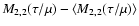
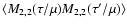
5.3 Stokes Q. The mean source function $\bar {S}_{2}$

We show in this section how to calculate the mean source function $\bar S_2(\tau)=\langle{\cal S}_{\rm Q}(\tau\vert{\mbox{\boldmath$\vec{H}$ }}\rangle$, where $\langle\ \rangle$ stand for the average over $P({\mbox{\boldmath$\vec{H}$ }})$. The two-scattering approximation applied to Eq. (41) yields

 

$${\cal S}_2(\tau\vert{\mbox{\boldmath$\vec{H}$ }})= (1-\epsilon_p)... ...mbox{\boldmath$\vec{H}$ }}) M_{2,2}(\cdot) C_{\rm I}(\tau')~{\rm d}\tau'\Bigr].$$ (47)

Averaging the primary source term in Eq. (47) is straightforward. To average the integral term, we must calculate the quantity $D_{2,2}(\varpi)$ defined by

$$D_{2,2}(\varpi) = \langle M_{2,2} {\rm e}^{\varpi~\nu\Pi_1}M_{2,2}\rangle,$$ (48)

where $\varpi=\vert\tau'-\tau\vert/\mu$ (see Eq. (42)). In the macroturbulent ($\nu=0$) and microturbulent ( $\nu\to \infty$) limits, $D_{2,2}(\varpi)$ becomes equal to $\langle M_{2,2}^2\rangle$and $\langle M_{2,2}\rangle^2$, respectively. We recall that in the microturbulent limit all the random coefficients can be replaced by their local averages over the magnetic field distribution. We now show that for a finite non zero value of $\nu$,

$$D_{2,2}(\varpi)= {\rm e}^{-\varpi~\nu}\langle M_{2,2}^2\rangle+ (1- {\rm e}^{-\varpi~\nu}) \langle M_{2,2}\rangle^2.$$ (49)

Observe that this result is simply a linear combination of the macro and microturbulent limits and is consistent with both limits.

We consider the Laplace transform of $D_{2,2}(\varpi)$ :

 

$$\tilde D_{2,2}(p) \int_0^\infty {\rm e}^{-p \varpi}D_{2,2}(\varpi)~{\rm d}\varpi,$$ =

$$\Bigl\langle M_{2,2}(p-\nu\Pi_1)^{-1}M_{2,2}\Bigr\rangle.$$ = (50)

The calculation of the inverse of the operator $(p-\nu\Pi_1)$ is equivalent to the solution of the integral equation

$$(p-\nu\Pi_1)f({\mbox{\boldmath$\vec{H}$ }})= g({\mbox{\boldmath$\vec{H}$ }}),$$ (51)

with f the unknown and g given. Here p is implicitly multiplied by the operator unity. Using Eq. (25), this integral equation can be written as

$$pf({\mbox{\boldmath$\vec{H}$ }}) + \nu f({\mbox{\boldmath$\ve... ...\mbox{\boldmath$\vec{H}$ }}'= g({\mbox{\boldmath$\vec{H}$ }}).$$ (52)

We first calculate the mean value of $f({\mbox{\boldmath$\vec{H}$ }})$ by averaging over ${\mbox{\boldmath$\vec{H}$ }}$. Inserting the result into Eq. (52), we obtain

$$f({\mbox{\boldmath$\vec{H}$ }})= {g({\mbox{\boldmath$\vec{H}$... ...boldmath$\vec{H}$ }}')~{\rm d}^3{\mbox{\boldmath$\vec{H}$ }'}.$$ (53)

Now we set g= M_2,2, multiply by M_2,2 and average over the magnetic field distribution (see Eq. (50)). A decomposition of $\nu/[p (\nu+p)]$ in simple fractions yields

$$\tilde D_{2,2}(p)= {1\over p+\nu}[\langle M_{2,2}^2\rangle- \langle M_{2,2}\rangle^2] + {1\over p}\langle M_{2,2}\rangle^2.$$ (54)

One sees immediately that $\tilde D_{2,2}(p)$ is the Laplace transform of the result given in Eq. (49).

A less general but more direct method for obtaining Eq. (49) is to expand the exponential operator in Eq. (48). This leads to

$$D_{2,2}(\varpi)= \left\langle M_{2,2}\left(1 - \varpi \nu \Pi... ...2}\varpi^2 \nu ^2 \Pi_1^2 + \ldots\right)M_{2,2}\right\rangle.$$ (55)

Using the properties of $\Pi_1$ given in Eqs. (26) and (27), we obtain

 

$$D_{2,2}(\varpi) = \langle M_{2,2}^2\rangle- \varpi \nu ~\left[\la... ...i^2 \nu ^2 \left[\langle M_{2,2}^2\rangle- \langle M_{2,2}\rangle^2\right] +...$$ (56)

Summing all the terms, we recover the result in Eq. (49).

So our final result for the mean source function is

 

$${\bar S_2(\tau)= (1-\epsilon_p)\langle M_{2,2}\rangle~C_{\rm I}(\tau)}$$

$$\qquad~+ ~(1-\epsilon_p)^2 \int_0^\infty\int_{x\mu}^{\rm wh} \varphi(x) \Psi_{2,2}(\mu)$$

$$\qquad~\times~\Bigl[{\rm e} ^{-\nu\vert\tau'-\tau\vert/\mu}[\langle M_{2,2}^2\rangle- \langle M_{2,2}\rangle^2 ] + \langle M_{2,2}\rangle^2\Bigr]$$

$$~\qquad\times~ {\rm e}^{-\vert\tau'-\tau\vert\varphi(x)/\mu}\varphi(x)C_{\rm I}(\tau')~{\rm d}\mu~{\rm d}x~{\rm d}\tau'.$$ (57)

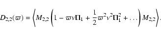
This expression involves only the primary source term $C_{\rm I}$defined in Eq. (37) and the mean values of M_2,2 and M_2,2².

As already pointed out, in the microturbulent and macroturbulent limits, the large square bracket reduces to $\langle M_{2,2}\rangle^2$ and $\langle M_{2,2}^2\rangle$, respectively. For a stationary Kubo-Anderson process m(t) of zero mean and density $\nu$, the covariance is given by (Brissaud & Frisch 1974)

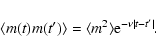$$\langle m(t)m(t')\rangle=\langle m^2\rangle{\rm e}^{-\nu\vert t-t'\vert}.$$ (58)

Replacing m(t) by the difference $M_{2,2}(\tau/\mu) -\langle M_{2,2}(\tau/\mu)\rangle$, we see that the square bracket, is simply the autocorrelation function $\langle M_{2,2}(\tau/\mu)M_{2,2}(\tau'/\mu)\rangle$. If we had considered ${\mbox{\boldmath$\vec{H}$ }}$ as a random process in space and not in time, i.e. if we had averaged Eq. (46) over the magnetic field distribution, there would be no factor $1/\mu$. This factor $1/\mu$ properly takes into account the number of turbulent eddies that are crossed along the line of sight.

We note also that for large values of $\vert\tau -\tau'\vert$ such that $\nu\vert\tau -\tau'\vert/\mu\gg 1$, the dominant factor inside the large square bracket in Eq. (57) is $\langle M_{2,2}\rangle^2$. So, as expected, we recover the microturbulent limit when many turbulent eddies lie between $\tau$ and $\tau'$.

Equation (57) shows also that $\bar {S}_{2}$ is independent of the correlation length of the magnetic field in the standard single scattering approximation since $\bar {S}_{2}$ is approximated by the first term in the r.h.s.

   
5.4 Mean Stokes Q

We are now ready to determine $\bar I_2(\tau,x,\mu)$, the average of the mean conditional polarization ${\cal I}_2(\tau,x,\mu\vert{\mbox{\boldmath$\vec{H}$ }})$ over the distribution of the magnetic field. Averaging Eq. (39), we obtain for $\bar I_2$ a standard transfer equation

$$\mu {\partial \bar I_2(\tau,x,\mu)\over \partial \tau}=\varphi(x)\Bigl[\bar I_2(\tau,x,\mu) - \bar S_2(\tau)\Bigr],$$ (59)

where $\bar S_2(\tau)$is given in Eq. (57). There is no contribution from the term involving the operator $\Pi_1$ since it becomes zero upon averaging (see Eq. (26)). The solution of Eq. (59) is of the form shown in Eqs. (28) and (29). For the surface value we simply have

$$\bar I_2(0,x,\mu)=\int_0^\infty {\rm e} ^{-\tau \varphi(x)/\mu} \bar S_2(\tau) \varphi(x)~{{\rm d}\tau\over\mu}\cdot$$ (60)

This expression is consistent with the fact that there is no randomness in the profile $\varphi$. The mean value of the azimuthal average of Stokes Q follows then from Eq. (3).

To summarize, the calculation of the mean value of ${\cal I}_2$ involves only a few fairly simple steps. First one has to solve a scalar transfer problem for I₁ with, say, an accelerated Lambda iteration method. Equation (57) gives an explicit expression for the mean source function $\bar {S}_{2}$ in which $C_{\rm I}$, the primary source, is given by Eq. (37). It suffices then to integrate the source function as shown in Eq. (60). Of course a choice has to be made for the distribution of the magnetic field.

The element M_2,2 can be written as (Stenflo 1994)

$$M_{2,2}= 1- 3 \sin^2\theta_{\rm B}\gamma_{\rm B}^2 \left[{\s... ... + {\cos^2\theta_{\rm B}\over 1+ \gamma_{\rm B}^2}\right]\cdot$$ (61)

Here, $\theta_{\rm B}$ is the inclination angle of the magnetic field and $\gamma_{\rm B}$ is a dimensionless parameter which depends on the intensity of the magnetic field. Namely, $\gamma_{\rm B}=2\pi\nu_{\rm L}g/\Gamma_{\rm T}$, with $\nu_{\rm L}=e \vert{\mbox{\boldmath$\vec{H}$ }}\vert/(4\pi mc)$ the Larmor frequency of the electron in the magnetic field, g the Landé factor of the upper level, $\Gamma_{\rm T}$ the destruction rate of the upper level alignment (sum of the radiative, inelastic and depolarizing destruction rates) (Bommier 1997a,b; Faurobert et al. 2001; Bommier et al. 2005). The element M_2,2does not depend on the longitude $\chi_{\rm B}$ of the magnetic field.

For a magnetic field with a constant intensity, isotropically distributed over the solid angle (Stenflo 1982; Landi Degl'Innocenti & Landi Degl'Innocenti 1988; LL04),

$$\langle M_{2,2} \rangle= {1\over 4\pi}\int_0^{2\pi}\int_0^\pi... ...\sin\theta_{\rm B}~ {\rm d}\theta_{\rm B}~{\rm d}\chi_{\rm B}.$$ (62)

A simple calculation yields

$$\langle M_{2,2} \rangle= 1-{2\over 5}\left[{\gamma_{\rm B}^2\... ... B}^2} + {4\gamma_{\rm B}^2\over 1+4\gamma_{\rm B}^2}\right],$$ (63)

and

$$\langle M_{2,2}^2 \rangle= 1- {4\over 35}{\gamma_{\rm B}^2\ov... ...^2)\over (1+4\gamma_{\rm B}^2)^2 (1+\gamma_{\rm B}^2)}\right].$$ (64)

One can verify that $\langle M_{2,2}^2\rangle$ is always positive.

   
5.5 Mean Stokes U

As shown by Eq. (4), Stokes U depends on I_k, $k=3,\ldots,6$, only. Proceeding as above, we introduce the mean conditional components ${\cal I}_k$ which satisfy the transfer Eq. (39) with the mean conditional source functions given by

 

$${\cal S}_k(\tau\vert{\mbox{\boldmath$\vec{H}$ }})=(1-\epsilon_p)M... ...{\rm 2}(\tau,x,\mu\vert{\mbox{\boldmath$\vec{H}$ }})~{\rm d}\mu~{\rm d}x\Bigg].$$ (65)

Now we remark that the square bracket can be expressed in terms of ${\cal S}_2(\tau\vert{\mbox{\boldmath$\vec{H}$ }})$ (see Eq. (40)). We thus obtain

$${\cal S}_k(\tau\vert{\mbox{\boldmath$\vec{H}$ }})= {M_{k,2}({... ...vec{H}$ }})}{\cal S}_2(\tau\vert{\mbox{\boldmath$\vec{H}$ }}).$$ (66)

Hence ${\cal S}_k$ is also given by Eq. (47) where M_2,2 is replaced by M_k,2 outside the square bracket. Averaging over the magnetic field as in Sect. 5.3, we obtain for $\bar S_k(\tau)= \langle{\cal S}_k(\tau\vert{\mbox{\boldmath$\vec{H}$ }})\rangle$ a result quite similar to Eq. (57), namely

 

$${\bar S_k(\tau)= (1-\epsilon_p)\langle M_{k,2}\rangle~C_{\rm I}(\tau)}$$

$$\qquad~+ \ (1-\epsilon_p)^2 \int_0^\infty\int_{x\mu}^{\rm wh}\varphi(x) \Psi_{2,2}(\mu) \Bigl[{\rm e} ^{-\nu\vert\tau'-\tau\vert/\mu}$$

$$\qquad~\times~[\langle M_{k,2}M_{2,2}\rangle- \langle M_{k,2}\rangle \langle M_{2,2}\rangle] + \langle M_{k,2}\rangle\langle M_{2,2}\rangle\Bigr]$$

$$\qquad~ \times~{\rm e}^{-\vert\tau'-\tau\vert\varphi(x)/\mu}\varphi(x)C_{\rm I}(\tau')~{\rm d}\mu~{\rm d}x~{\rm d}\tau'.$$ (67)

In the first term $\langle M_{k,2}\rangle$ replaces $\langle M_{2,2}\rangle$ and in the square bracket we have combinations of the macroturbulent and microturbulent limits of the product M_k,2M_2,2.

At the surface, the mean values $\bar I_k(0,x,\mu)$ are simply given by Eq. (60) with $\bar {S}_{2}$ replaced by $\bar S_k$. The M_k,2 depend linearly on $\sin \chi_{\rm B}$ and $\cos \chi_{\rm B}$. Hence the mean values of $\langle M_{k,2}\rangle$ and $\langle M_{k,2}M_{2,2}\rangle$ over an isotropically distributed field are zero (see Eq. (62)) and Stokes U is zero as it should be. The same situation holds for any axisymmetric magnetic field distribution.

   
5.6 Line core and line wings

Since the Hanle effect acts only in the line core, the conditional source functions ${\cal S}_{2}$ and ${\cal S}_k$ are actually function of the frequency x. The expressions given in Eqs. (57) and (67) must then be somewhat modified. In the first term which serves as primary source, M₂₂ must be set to unity and M_k2to zero when $\vert x\vert>x_{\rm c}$. In the integral term, the coefficient M₂₂must be set to unity and the coefficient M_k2 to zero when $\vert x'\vert>x_{\rm c}$.

   
6 The Hanle effect with turbulent velocity and magnetic fields

We now consider the joint effects of a turbulent velocity field ${\mbox{\boldmath$\vec{v}$ }}$ and of a turbulent magnetic field ${\mbox{\boldmath$\vec{H}$ }}$. We assume that the velocity field has the same statistical properties as the magnetic field, namely that it is also a KAP with density $\nu$ and that it has the same jumping points as the magnetic field. We denote by $P_{\rm H,v}({\mbox{\boldmath$\vec{H}$ }},{\mbox{\boldmath$\vec{v}$ }})$ the joint probability density of ${\mbox{\boldmath$\vec{H}$ }}$and ${\mbox{\boldmath$\vec{v}$ }}$ and by $P_{\rm H}({\mbox{\boldmath$\vec{H}$ }})$ and $P_{\rm v}({\mbox{\boldmath$\vec{v}$ }})$the marginal density probability of ${\mbox{\boldmath$\vec{H}$ }}$ and ${\mbox{\boldmath$\vec{v}$ }}$, respectively. An effective medium approximation will be introduced to handle the complexity introduced by the turbulent field, otherwise the method follows the same lines as above.

The operator of the full random Markov process is

 

$$\Pi({\mbox{\boldmath$\vec{H}$ }},{\mbox{\boldmath$\vec{v}$ }};{\m... ... P_{\rm H,v}({\mbox{\boldmath$\vec{H}$ }},{\mbox{\boldmath$\vec{v}$ }})\right].$$ (68)

Because of the Doppler effect, the random field ${\mbox{\boldmath$\vec{v}$ }}$ enters in the absorption profile which becomes $\varphi(x-{\mbox{\boldmath$\vec{v}$ }}\cdot{\mbox{\boldmath$\vec{\Omega}$ }}/c)$, with ${\mbox{\boldmath$\vec{\Omega}$ }}$ the direction of propagation of the radiation. Proceeding as above, we consider the magnetic field and velocity field to be random processes in time. We introduce the joint process $\{{\mbox{\boldmath$\vec{H}$ }}(t),{\mbox{\boldmath$\vec{v}$ }}(t),{\mbox{\boldmath$\vec{I}$ }}(t)\}$ and its probability density ${\cal P}({\mbox{\boldmath$\vec{H}$ }},{\mbox{\boldmath$\vec{v}$ }},{\mbox{\boldmath$\vec{I}$ }};t)$ which satisfies

$${\partial {\cal P}\over\partial t}= \Pi{\cal P} -c \sum_{l=1}... ...} + {\cal A({\mbox{\boldmath$\vec{v}$ }})}G_l] {\cal P}\Bigr],$$ (69)

with the initial condition

$${\cal P}({\mbox{\boldmath$\vec{H}$ }},{\mbox{\boldmath$\vec{v... ...box{\boldmath$\vec{v}$ }}) \prod_{l=1}^6\delta(I_l-I_l^{(0)}).$$ (70)

We introduce the mean conditional irreducible Stokes vector ${\mbox{\boldmath$\vec{\cal I}$ }}(t,z,x,\mu\vert{\mbox{\boldmath$\vec{H}$ }},{\mbox{\boldmath$\vec{v}$ }})$. Each component is defined as in Eq. (16) with $P({\mbox{\boldmath$\vec{H}$ }})$ replaced by $P_{\rm H,v}({\mbox{\boldmath$\vec{H}$ }},{\mbox{\boldmath$\vec{v}$ }})$. The stationary solution of the time-dependent transfer equation for ${\mbox{\boldmath$\vec{\cal I}$ }}$satisfies a set of equations similar to Eqs. (22) and (23) where $\varphi(x)$ is replaced by $\varphi(x-{\mbox{\boldmath$\vec{v}$ }}\cdot{\mbox{\boldmath$\vec{\Omega}$ }}/c)$. The integral equation corresponding to Eq. (30) is

 

$${\mbox{\boldmath$\vec{\cal S}$ }}(\tau\vert{\mbox{\boldmath$\vec{... ...{v}$ }}){\mbox{\boldmath$\vec{\cal S}$ }}(\tau'\vert~\cdot,\cdot)~{\rm d}\tau',$$ (71)

where the operator ${\cal K}^{\rm H,v}$ is defined by

 

$${\cal K}^{\rm H,v}(\tau;{\mbox{\boldmath$\vec{H}$ }},{\mbox{\bold... ...au\vert\over \mu}(\varphi - \nu\Pi_1)\right]\varphi(\cdot)~{\rm d}\mu~{\rm d}x.$$ (72)

As above, conditional means are denoted with calligraphic upper case letters. The notation $\int_{x\mu}^{\rm wh}$ is defined in Eq. (32). The dots indicates that $\varphi$ and ${\mbox{\boldmath$\vec{\cal S}$ }}$ are functions of the velocity and magnetic fields variables. In the exponential, $\varphi$ stands for $\varphi(x-{\mbox{\boldmath$\vec{v}$ }}\cdot{\mbox{\boldmath$\vec{\Omega}$ }}/c)$ times the operator unity. The operator $\Pi_1$ is defined by

 

$$\Pi_1({\mbox{\boldmath$\vec{H}$ }},{\mbox{\boldmath$\vec{v}$ }}\v... ...\Bigr]P_{\rm H,v}({\mbox{\boldmath$\vec{H}$ }'},{\mbox{\boldmath$\vec{v}$ }'}).$$ (73)

To simplify the notation, we now introduce the symbol

$$\Big\langle\ldots\Big\rangle_{\rm v}= \int P_{\rm v}({\mbox{\... ...math$\vec{v}$ }})\ldots {\rm d}^3{\mbox{\boldmath$\vec{v}$ }},$$ (74)

the variable

$$x_{\rm d}= x- {1\over c}{\mbox{\boldmath$\vec{v}$ }}\cdot{\mbox{\boldmath$\vec{\Omega}$ }},$$ (75)

and the operator

$${\cal O}(\tau,\mu;\varphi,\Pi_1) =\exp\left[-{\vert\tau\vert\over \mu}(\varphi(x_{\rm d}) - \nu\Pi_1)\right].$$ (76)

We also introduce $\Pi_1^{\rm v}$, the projection of $\Pi_1$ on functions independent of the magnetic field. It can be written as

$$\Pi_1^{\rm v}= - {1\over P_{\rm v}({\mbox{\boldmath$\vec{v}$ ... ...ldmath$\vec{v}$ }})] P_{\rm v}({\mbox{\boldmath$\vec{v}$ }'}).$$ (77)

We now show how to establish explicit expressions for the mean values of the six components of the source vector ${\mbox{\boldmath$\vec{\cal S}$ }}$. In addition to approximations described in Sect. 4, an effective medium is introduced to handle some of the random velocity field effects.

   
6.1 Stokes I; effective medium approximation

With the above assumptions, the component ${\cal S}_1$ is independent of the magnetic field and we recover the problem treated in FF76. The integral equation for ${\cal S}_1(\tau\vert{\mbox{\boldmath$\vec{v}$ }})$ is

 

$${\cal S}_1(\tau\vert{\mbox{\boldmath$\vec{v}$ }})= G_1(\tau) + ~ ... ...u-\tau';{\mbox{\boldmath$\vec{v}$ }}){\cal S}_1(\tau'\vert~\cdot)~{\rm d}\tau'.$$ (78)

Here the operator ${\cal K}^{\rm v}_{1,1}$ is defined as in Eq. (72) with $\Pi_1$ replaced by $\Pi_1^{\rm v}$ and $\hat\Psi$ replaced by $\Psi_{11}=1$.

An effective source function, independent of the velocity field was introduced in FF76 on the ground that the source function is rather insensitive to turbulent fields (Athay 1972). This point is discussed again below. So we make the approximation,

$${\cal S}_1(\tau\vert{\mbox{\boldmath$\vec{v}$ }})= {\cal S}^{\rm eff}_1(\tau),$$ (79)

and use it as an Ansatz in Eq. (78). Since the integral term still depends on ${\mbox{\boldmath$\vec{v}$ }}$, we average it over the velocity distribution (see Sect. 8 in FF76). This procedure leads to the integral equation

$${\cal S}^{\rm eff}_1(\tau) = G_1(\tau) + (1-\epsilon_o)\int_0... ...\rm eff}(\tau-\tau'){\cal S}^{\rm eff}_1(\tau')~{\rm d}\tau',$$ (80)

with

$${\cal K}_{1,1}^{\rm eff}(\tau)=\int_{x\mu}^{\rm wh}\Big\lang... ...v}) \varphi(~\cdot~)\Big\rangle_{\rm v}~{\rm d}\mu~{\rm d}x.$$ (81)

A numerical method for the calculation of the effective source function is described in FF80.

   
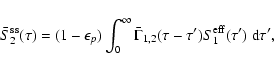
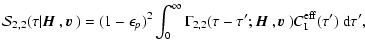
6.2 Stokes Q; mean source function

We deduce from Eq. (71) that ${\cal S}_2(\tau\vert{\mbox{\boldmath$\vec{H}$ }}, {\mbox{\boldmath$\vec{v}$ }})$ satisfies an integral equation which can be written

$${\cal S}_2(\tau\vert{\mbox{\boldmath$\vec{H}$ }},{\mbox{\bold... ...ert{\mbox{\boldmath$\vec{H}$ }},{\mbox{\boldmath$\vec{v}$ }}),$$ (82)

where

 

$${\cal S}_{1,2}(\tau\vert{\mbox{\boldmath$\vec{H}$ }},{\mbox{\bold... ...c{H}$ }},{\mbox{\boldmath$\vec{v}$ }}){\cal S}_1(\tau'\vert\cdot)~{\rm d}\tau',$$ (83)

plays the role of a primary source term and where

 

$${\cal S}_{2,2}(\tau\vert{\mbox{\boldmath$\vec{H}$ }},{\mbox{\bold... ...}},{\mbox{\boldmath$\vec{v}$ }}){\cal S}_2(\tau'\vert\cdot,\cdot)~{\rm d}\tau',$$ (84)

is the integral term. In the single scattering approximation, ${\cal S}_{2}$ reduces to ${\cal S}_{1,2}$. Here ${\cal K}_{1,2}^{\rm v,H}$ and ${\cal K}_{2,2}^{\rm v,H}$ are defined as in Eq. (72), with $\hat\Psi$ replaced by $\Psi_{1,2}$ and $\Psi_{2,2}$, respectively. The integral equation for ${\cal S}_{2}$ is now solved with a first order Neumann series expansion (see Sect. 5.2) and the solution is averaged over the magnetic and velocity field distribution to obtain the mean value $\bar S_2(\tau)=\langle{\cal S}_2({\mbox{\boldmath$\vec{H}$ }},{\mbox{\boldmath$\vec{v}$ }})\rangle$. We first deal with ${\cal S}_{1,2}$ and then with  ${\cal S}_{2,2}$.

   
6.2.1 Evaluation and mean value of ${\cal S}_{1,2}$

For consistency with the effective medium approximation used to evaluate Stokes I, we replace in Eq. (83) ${\cal S}_1(\tau\vert\cdot)$ by $S_1^{\rm eff}(\tau)$ and thus obtain

 

$${\cal S}_{1,2}(\tau\vert{\mbox{\boldmath$\vec{H}$ }},{\mbox{\bold... ...c{H}$ }},{\mbox{\boldmath$\vec{v}$ }}){\cal S}_1^{\rm eff}(\tau')~{\rm d}\tau',$$ (85)

with

 

$$\Gamma_{1,2}(\tau;{\mbox{\boldmath$\vec{H}$ }},{\mbox{\boldmath$\... ... d}){\cal O}(\tau,\mu;\varphi,\Pi_1^{\rm v})\varphi(\cdot)~{\rm d}\mu~{\rm d}x.$$ (86)

Proceeding as in Sect. 5.3, we calculate the Laplace transform of $\Gamma_{1,2}$. It may be written as

 

$$\tilde\Gamma_{1,2}(p;{\mbox{\boldmath$\vec{H}$ }},{\mbox{\boldmath$\vec{v}$ }}) M_{2,2}({\mbox{\boldmath$\vec{H}$ }}) \int_{\rm x\mu}^{\rm wh}\Psi_{1,2}(\mu) \Bigg\{{\varphi ^2\over p + (\varphi + \nu)/\mu}$$ =

$$+ {\nu\over\mu}{\varphi\over p + (\varphi + \nu)/\mu} \Bigl\langle{\varphi \over p + (\varphi + \nu)/\mu}\Bigr\rangle_{\rm v}$$

$$\times\left[\Bigl\langle1-{\nu\over\mu}{1\over p + (\varphi + \nu)/\mu}\Bigr\rangle_{\rm v}\right]^{-1} \Bigg\}~{\rm d}\mu~{\rm d}x,$$ (87)

where $\varphi$ stands for $\varphi(x-{\mbox{\boldmath$\vec{v}$ }}\cdot{\mbox{\boldmath$\vec{\Omega}$ }}/c)$.

Now we remark that the integration over x plays a role somewhat similar to an averaging over the velocity field. When $\nu=0$ ( macroturbulent limit), an integration over x is exactly equivalent to an integration over ${\mbox{\boldmath$\vec{v}$ }}$. It is not true when $\nu$ is finite. This remark, which explains why the source function, in the scalar case, is not very sensitive to turbulent velocities, suggests to introduce for ${\cal S}_{1,2}$ an effective medium approximation, namely

$${\cal S}_{1,2}(\tau;{\mbox{\boldmath$\vec{H}$ }},{\mbox{\bold... ...{2,2}({\mbox{\boldmath$\vec{H}$ }})C_{\rm I}^{\rm eff}(\tau),$$ (88)

with

$$C_{\rm I}^{\rm eff}(\tau)=\int_0^\infty{\cal K}_{1,2}^{\rm eff}(\tau-\tau'){\cal S}^{\rm eff}_1(\tau')~{\rm d}\tau',$$ (89)

and

 

$${\cal K}_{1,2}^{\rm eff}(\tau)=\int_{x\mu}^{\rm wh} \Psi_{1,2}(\m... ...\varphi,\Pi_1^{\rm v}) \varphi(~\cdot~)\Big\rangle_{\rm v}~{\rm d}\mu~{\rm d}x.$$ (90)

In the macro and micro turbulent limits, ${\cal K}_{1,2}^{\rm eff}$reduces to the usual deterministic K_1,2 with either the frequency profile $\varphi$ or its mean value $\langle\varphi\rangle$ over the velocity distribution. In these limits the integral of K_1,2 over $\tau$ (from $-\infty$ to $+\infty$) is zero. This property holds also for ${\cal K}_{1,2}^{\rm eff}$. It is a consequence of the fact that the integral of $\Psi_{1,2}$ over $\mu$ is zero.

The effective medium approximation cannot take into account any sort of coupling between magnetic field and velocity field fluctuations. We show now that one can construct an approximation of ${\cal S}_{1,2}$based on the macro and microturbulent limits of $\Gamma_{1,2}$ which does not have this drawback.

The inverse Laplace transform in Eq. (87) cannot be calculated explicitely, however one can easily obtain the macro ($\nu=0$) and microturbulent ( $\nu=\infty$) limits,

 

$$\Gamma_{1,2}(\tau; {\mbox{\boldmath$\vec{H}$ }},{\mbox{\boldmath$... ...(x_{\rm d}){\rm e}^{-\vert\tau\vert\varphi(x_{\rm d})/\mu}~{\rm d}\mu~{\rm d}x,$$ (91)

 

$$\Gamma_{1,2}(\tau; {\mbox{\boldmath$\vec{H}$ }},{\mbox{\boldmath$... ...i\rangle{\rm e}^{-\vert\tau\vert\langle\varphi\rangle/\mu}~{\rm d}\mu~{\rm d}x.$$ (92)

Note that these limits still depend on the random values of ${\mbox{\boldmath$\vec{H}$ }}$and ${\mbox{\boldmath$\vec{v}$ }}$. A numerical investigation of the effective kernel $K_{1,1}^{\rm eff}$ (FF80) shows that it behaves as the microturbulent limit for optical depths larger than $1/\nu$ and like that the macroturbulent limit for optical depths smaller than $10^{-2}/\nu$ with a smooth transition between the two limits. Also the exact expression for obtained $D_{2,2}(\varpi)$ in Eq. (49) is a combination of the macro and microturbulent limits. We propose the approximation

 

$$\Gamma_{1,2}(\tau;{\mbox{\boldmath$\vec{H}$ }},{\mbox{\boldmath$\... ...\boldmath$\vec{v}$ }})_{\rm mi}\left(1-{\rm e}^{-\nu\vert\tau\vert/\mu}\right).$$ (93)

It is consistent with the exact result in Eq. (49) obtained for the pure magnetic field case. It should be possible to improve this approximation by expanding $\tilde \Gamma_{1,2}(p;{\mbox{\boldmath$\vec{H}$ }},{\mbox{\boldmath$\vec{v}$ }})$ in powers of $\nu$ for $\nu\to 0$ and in powers of $1/\nu$ for $\nu\to \infty$.

We now average ${\cal S}_{1,2}(\tau\vert{\mbox{\boldmath$\vec{H}$ }},{\mbox{\boldmath$\vec{v}$ }})$ over the joint magnetic and velocity field distribution to obtain the mean source function in the single scattering approximation denoted here by $\bar S_2^{\rm ss}(\tau)$. We consider separately each of the two approximations constructed for ${\cal S}_{1,2}$. The effective medium approximation leads to

$$\bar S_2^{\rm ss}(\tau)= (1-\epsilon_p)\langle M_{2,2}({\mbox... ...{1,2}^{\rm eff}(\tau -\tau')S_1^{\rm eff}(\tau')~{\rm d}\tau',$$ (94)

where $K_{1,2}^{\rm eff}$ is defined in Eq. (90). The second approximation, which can account for correlations between the velocity and magnetic field distributions, yields

$$\bar S_2^{\rm ss}(\tau)= (1-\epsilon_p)\int_0^\infty \bar\Gamma_{1,2}(\tau -\tau')S_1^{\rm eff}(\tau')~{\rm d}\tau',$$ (95)

where

 

$$\bar\Gamma_{1,2}(\tau) \int_{\rm x\mu}^{\rm wh}\Psi_{1,2}(\mu)\Bigl\{ \langle M_{2,2}\va... ...2 {\rm e}^{-\vert\tau\vert\varphi/\mu}\rangle ~{\rm e}^{-\nu\vert\tau\vert/\mu}$$ =

$$+~\langle M_{2,2}\varphi\rangle\langle\varphi\rangle {\rm e}^{-\v... ...mu}~\left(1-{\rm e}^{-\nu\vert\tau\vert/\mu}\right)\Bigr\}~{\rm d}\mu~{\rm d}x.$$ (96)

In Eqs. (94) and (96), the average of M_2,2 is over the magnetic field distribution function $P_{\rm H}({\mbox{\boldmath$\vec{H}$ }})$, the average of $\varphi$ is over the velocity distribution function $P_{\rm v}({\mbox{\boldmath$\vec{v}$ }})$ and for the quantities which depend on ${\mbox{\boldmath$\vec{H}$ }}$ and ${\mbox{\boldmath$\vec{v}$ }}$, the averages are over the joint magnetic and velocity distribution function $P({\mbox{\boldmath$\vec{H}$ }}, {\mbox{\boldmath$\vec{v}$ }})$. It should be noted that the second approximation reduces to an approximate version of the first one if $P({\mbox{\boldmath$\vec{H}$ }}, {\mbox{\boldmath$\vec{v}$ }})$ can be factorized as a product $P({\mbox{\boldmath$\vec{H}$ }}, {\mbox{\boldmath$\vec{v}$ }})=P_{\rm v}({\mbox{\boldmath$\vec{v}$ }})P_{\rm H}({\mbox{\boldmath$\vec{H}$ }})$. We note also that the integral over $\tau$ of $\bar\Gamma_{1,2}$ is zero, as is the integral of $K_{1,2}^{\rm eff}$.

   
6.2.2 Evaluation and mean value of ${\cal S}_{2,2}$

To calculate ${\cal S}_{2,2}$ we should in principle replace in Eq. (84) ${\cal S}_2(\tau\vert{\mbox{\boldmath$\vec{H}$ }}, {\mbox{\boldmath$\vec{v}$ }})$ by ${\cal S}_{1,2}(\tau\vert{\mbox{\boldmath$\vec{H}$ }},{\mbox{\boldmath$\vec{v}$ }})$. Here we use the approximate value ${\cal S}_{1,2}^{\rm eff}(\tau\vert{\mbox{\boldmath$\vec{H}$ }})$ given in Eq. (88). With the full expression the algebra would become unnecessary complicated for a term which can be considered as a correction to ${\cal S}_{1,2}$ since the single scattering albedo $\lambda_2$ is smaller than unity (see Sect. 5.2). We thus obtain

 

$${\cal S}_{2,2}(\tau\vert{\mbox{\boldmath$\vec{H}$ }}, {\mbox{\bol... ...{H}$ }}, {\mbox{\boldmath$\vec{v}$ }}) C_{\rm I}^{\rm eff}(\tau')~{\rm d}\tau',$$ (97)

with

 

$$\Gamma_{2,2}(\tau;{\mbox{\boldmath$\vec{H}$ }},{\mbox{\boldmath$\... ...cal O}(\tau,\mu;\varphi,\Pi_1)M_{2,2}(\cdot)\varphi(\cdot)~{\rm d}\mu~{\rm d}x.$$ (98)

We now consider the Laplace transform of $\Gamma_{2,2}$. To calculate the action of the operator $\Bigl[p + (\varphi - \nu\Pi_1)/\mu\Bigr]^{-1}$ we proceed as in Sect. 5.3, i.e. we look for the solution of the integral equation

$$\left[p + (\varphi - \nu\Pi_1)/\mu\right]f({\mbox{\boldmath... ...\mbox{\boldmath$\vec{H}$ }})g_2({\mbox{\boldmath$\vec{v}$ }}),$$ (99)

where $g_1({\mbox{\boldmath$\vec{H}$ }})$ and $g_2({\mbox{\boldmath$\vec{v}$ }})$ are given functions and $f({\mbox{\boldmath$\vec{H}$ }},{\mbox{\boldmath$\vec{v}$ }})$ the unknown. After some simple algebra, we find

 

$$\tilde\Gamma_{2,2}(p;{\mbox{\boldmath$\vec{H}$ }},{\mbox{\boldmath$\vec{v}$ }}) M_{2,2}({\mbox{\boldmath$\vec{H}$ }})\int_{\rm x\mu}^{\rm wh}\Psi_{2,2}(\mu) \Bigg\{{M_{2,2}\varphi ^2\over p + (\varphi + \nu)/\mu}$$ =

$$+ {\nu\over\mu}{\varphi\over p + (\varphi + \nu)/\mu} \Bigl\langle{M_{2,2}\varphi \over p + (\varphi + \nu)/\mu}\Bigr\rangle_{\rm H,v}$$

$$\times \left[\Bigl\langle1-{\nu\over\mu}{1\over p + (\varphi + \nu)/\mu}\Bigr\rangle_{\rm v}\right]^{-1} \Bigg\}~{\rm d}\mu~{\rm d}x.$$ (100)

This expression is similar to Eq. (87) but is quadratic in M_2,2. Its limits for $\nu=0$ and $\nu=\infty$ are

 

$$\Gamma_{2,2}(\tau; {\mbox{\boldmath$\vec{H}$ }},{\mbox{\boldmath$... ...x_{\rm d}){\rm e} ^{-\vert\tau\vert\varphi(x_{\rm d})/\mu}~{\rm d}\mu~{\rm d}x,$$ (101)

 

$$\Gamma_{2,2}(\tau; {\mbox{\boldmath$\vec{H}$ }},{\mbox{\boldmath$... ...{\rm v} {\rm e}^{-\vert\tau\vert\langle\varphi\rangle/\mu}~{\rm d}\mu~{\rm d}x.$$ (102)

With these two limits, one can construct an approximate expression for the mean value $\bar \Gamma_{2,2}(\tau)$ with the procedure applied in Eq. (93) to $\bar \Gamma_{1,2}(\tau)$.

Collecting all the results, we obtain

$$\bar S_{2}(\tau)= \bar S_{2}^{\rm ss}(\tau) + (1-\epsilon_p)^... ...mma_{2,2}(\tau-\tau') C_{\rm I}^{\rm eff}(\tau')~{\rm d}\tau',$$ (103)

where $\bar S_{2}^{\rm ss}$ is given by Eqs. (94) or (95) and

 

$$\bar\Gamma_{2,2}(\tau) \int_{\rm x\mu}^{\rm wh}\Psi_{2,2}(\mu)\Bigl\{ \langle M_{2,2}^2\... ...2 {\rm e}^{-\vert\tau\vert\varphi/\mu}\rangle ~{\rm e}^{-\nu\vert\tau\vert/\mu}$$ =

$$+\langle M_{2,2}\varphi\rangle^2 {\rm e}^{-\vert\tau\vert\langle\... ...hi\rangle/\mu}~(1-{\rm e}^{-\nu\vert\tau\vert/\mu})\Bigr\}~{\rm d}\mu~{\rm d}x.$$ (104)

This expression takes a simpler form if the distribution function $P({\mbox{\boldmath$\vec{H}$ }}, {\mbox{\boldmath$\vec{v}$ }})$ can be factorized since one can average M_2,2 and $\varphi$ independently. If $\varphi$ is not random, one recovers the expression given for $\bar {S}_{2}$ in Eq. (57).

   
6.3 Stokes U. Mean source function

The expressions given in Sect. 5.5 are easily generalized to the random velocity case. The ${\cal I}_k(\tau,x,\mu\vert{\mbox{\boldmath$\vec{H}$ }},{\mbox{\boldmath$\vec{v}$ }})$ (k=3 to 6) satisfy the transfer Eq. (39) with ${\cal I}_2$ replaced by ${\cal I}_k$ and ${\cal S}_{2}$ replaced by

$${\cal S}_k(\tau\vert{\mbox{\boldmath$\vec{H}$ }},{\mbox{\bold... ...box{\boldmath$\vec{H}$ }},{\mbox{\boldmath$\vec{v}$ }})\bigr],$$ (105)

where ${\cal S}_{1,2}$ and ${\cal S}_{2,2}$ are defined in Eqs. (83) and (84). The expression of ${\cal S}_k$ is a straightforward generalization of Eqs. (65) and (66).

To calculate the mean value of ${\cal S}_k$, we follow the procedure described in Sect. 6.2. Replacing ${\cal S}_{1,2}$ by ${\cal S}_{1,2}^{\rm eff}$, we obtain

 

$$\bar S_k(\tau)=(1-\epsilon_p)\langle M_{2,2}\rangle C_{\rm I}^{\r... ...^\infty \bar \Gamma_{k,2}(\tau -\tau') C_{\rm I}^{\rm eff}(\tau')~{\rm d}\tau',$$ (106)

where

 

$$\bar\Gamma_{k,2}(\tau) \int_{\rm x\mu}^{\rm wh}\Psi_{2,2}(\mu) \Bigl\{\langle M_{k,2}M_{... ...2 {\rm e}^{-\vert\tau\vert\varphi/\mu}\rangle ~{\rm e}^{-\nu\vert\tau\vert/\mu}$$ =

$$+\langle M_{k,2}\varphi\rangle\langle M_{2,2}\varphi\rangle {\rm ... ...hi\rangle/\mu}~(1-{\rm e}^{-\nu\vert\tau\vert/\mu})\Bigr\}~{\rm d}\mu~{\rm d}x.$$ (107)

If $\varphi$ is not random, we recover the expression given in Eq. (67).

   
6.4 Mean Stokes parameters

The mean conditional six-component vector ${\mbox{\boldmath$\vec{\cal I}$ }}(\tau,x,\mu\vert{\mbox{\boldmath$\vec{H}$ }},{\mbox{\boldmath$\vec{v}$ }})$ is given by Eqs. (28) and (29) with $\varphi(x)$ replaced by $\varphi(x-{\mbox{\boldmath$\vec{v}$ }}\cdot{\mbox{\boldmath$\vec{\Omega}$ }}/c)$ and ${\mbox{\boldmath$\vec{\cal S}$ }}(\tau\vert{\mbox{\boldmath$\vec{H}$ }})$ by ${\mbox{\boldmath$\vec{\cal S}$ }}(\tau\vert{\mbox{\boldmath$\vec{H}$ }},{\mbox{\boldmath$\vec{v}$ }})$. The averaging over the magnetic field and velocity field distributions cannot be performed explicitly unless we replace each component of ${\mbox{\boldmath$\vec{\cal S}$ }}(\tau\vert{\mbox{\boldmath$\vec{H}$ }},{\mbox{\boldmath$\vec{v}$ }})$ by the mean source functions ${\bar S}_k(\tau)$, $k=1\ldots6$, constructed above (for k=1, the mean source function is $S_1^{\rm eff}(\tau)$). With this approximation, the six components of the mean irreducible Stokes vector at $\tau=0$ can be written as

$$\bar I_{k}^{\rm eff}(0,x,\mu) =\int_0^\infty K_2^{\rm eff}(\tau,x,\mu) \bar S_{k}(\tau)~{{\rm d}\tau\over\mu},$$ (108)

with

$$K_2^{\rm eff}(\tau,x,\mu)= \Big\langle \exp\Bigl[-{\vert\tau... ... \nu\Pi_1^{\rm v})\Bigr] \varphi(~\cdot~)\Big\rangle_{\rm v}.$$ (109)

The operator $\Pi_1^{\rm v}$ is defined in Eq. (77). The mean source functions are given in Eq. (80) for k=1, in Eq. (103) for k=2 and in Eq. (106) for the other values of k. The function $K_2^{\rm eff}(\tau,x,\mu)$ is the effective escape probability introduced in FF76. A numerical method for the calculation of $K_2^{\rm eff}$ based on an exponential representation is described in FF80. The mean values of Q and Ucan then be deduced from Eqs. (3) and (4).

In this section we have treated simultaneously the effects of a turbulent velocity field and of a turbulent magnetic field, both represented by KAPs. The magnetic field effects were treated with the same approximations as in the absence of velocity field. Namely, we have neglected the effect of the magnetic field on Stokes I, the coupling of Stokes Q with Stokes U and we have calculated the polarization with a two-scattering approximation. For the Stokes parameter I, we have introduced an effective source function which takes into account finite correlation length effects of the velocity field and allows one to separate some of the velocity field from the magnetic field effects. We have thus been able to construct explicit expressions for the mean Stokes parameters Q and U which take into account finite correlation length effects and also correlations between the magnetic field and velocity field fluctuations. In the model we have used, the velocity field and magnetic field have the same correlation length and the same jumping points. It is certainly possible to release these assumption. For instance, in Brissaud & Frisch (1971), the electronic and ionic microfields of the stochastic Stark effect are represented by two KAPs with different correlation lengths.

   
7 Concluding remarks

In this paper, we have given explicit expressions for the mean observable Stokes parameters. We defer to a subsequent work the numerical calculation of these mean Stokes parameters. The results will depend on the choices made for the velocity field and magnetic field distribution function. The current views on solar magnetic fields (Stenflo 2004) is that 1% of the photospheric volume is filled by kG flux tubes while 99% is filled with a small scale turbulent field with a strength in the range of tens of Gauss. Magnetograms from the Swedish La Palma telescope and from MDI indicate that the probability distribution function (PDF) of the magnetic field strengths can be well fitted by Voigt functions with dispersion (damping) wings that extend out to kG fields (Stenflo & Holzreuter 2002, 2003). For scales below the diffraction limit of present day telescopes (about 100 km), numerical simulations of magneto-convection or fully developed turbulence can provide the PDF of the magnetic field strength, but also the distribution of the magnetic field directions and some indications on typical correlation scales. Numerical simulations may also provide some informations on the velocity distribution and on the correlations between velocity and magnetic field fluctuations. We note that our model should be able to incorporate an anisotropic distribution of magnetic fields and also a correlation scale depending on a mean magnetic field strength.

Acknowledgements

I have greatly benefited from discussions with Dr. V. Bommier, M. Faurobert and J. Stenflo. This research was supported by the Indo-French Center for the Promotion of Advanced Research (IFCPAR 2404-2).

References

• Anderson, P. W. 1954, J. Phys. Soc. Jpn 9, 316 (In the text)
• Athay, G. 1972, Radiation Transport in Spectral Lines (Dordrecht, Holland: Reidel Publishing Company) (In the text)
• Auvergne, M., Frisch, H., Frisch, U., Froeschlé, Ch., & Pouquet, A. 1973, A&A, 29, 93 [NASA ADS] (In the text)
• Barucha-Reid, A. T. 1960, Elements of the Theory of Markov Processes and their Applications (New York: McGraw-Hill) (In the text)
• Bommier, V. 1997a, A&A, 328, 706 [NASA ADS] (In the text)
• Bommier, V. 1997b, A&A, 328, 726 [NASA ADS]
• Bommier, V., Derouich, M., Landi Degl'Innocenti, E., Molodij, G., & Sahal-Bréchot, S. 2005, A&A, 432, 295 [EDP Sciences] [NASA ADS] [CrossRef] (In the text)
• Brissaud, A., & Frisch, U. 1971, J. Quant. Spec. Radiat. Transf., 11, 1767 (In the text)
• Brissaud, A., & Frisch, U. 1974, J. Math. Phys., 15, 524 [CrossRef] (In the text)
• Domke, H., & Hubeny, I. 1988, ApJ, 213, 296
• Domke, H., & Pavlov, G. G. 1979, Ap&SS, 66, 47 [NASA ADS] (In the text)
• Faurobert-Scholl, M. 1991, A&A, 246, 469 [NASA ADS] (In the text)
• Faurobert-Scholl, M. 1993, A&A, 268, 765 [NASA ADS] (In the text)
• Faurobert-Scholl, M. 1996, Sol. Phys. 164, 79 (In the text)
• Faurobert, M., Arnaud, J., Vigneau, J., & Frisch, H. 2001, A&A, 378, 627 [EDP Sciences] [NASA ADS] [CrossRef] (In the text)
• Feller, W. 1971, An Introduction to probability theory and its applications, Vol. II, Second edition (New York: John Wiley and Sons Inc.) (In the text)
• Frisch, H. 1998, A&A, 338, 683 [NASA ADS] (In the text)
• Frisch, H. 1999, in ASSL Series 243, Solar Polarization, ed. K. N. Nagendra, & J. O. Stenflo, 97 (F99) (In the text)
• Frisch, H., & Frisch, U. 1976, MNRAS, 175, 157 [NASA ADS] (FF76) (In the text)
• Frisch, U. 1968, in Probabilistic Methods in Applied Mathematics, ed. A. T. Bharucha-Reid (New York: Academic Press), 75 (In the text)
• Frisch, U., & Brissaud, A. 1971, J. Quant. Spec. Radiat. Trans., 11, 1753 (In the text)
• Froeschlé, Ch., & Frisch, H. 1980, A&A, 91, 202 [NASA ADS] (FF80)
• Gail, H. P., Sedlmayr, E., & Traving, G. 1975, A&A, 44, 421 [NASA ADS] (In the text)
• Holzreuter, R., Fluri, D. M., & Stenflo. J. O. 2005, A&A, 434, 713 [EDP Sciences] [NASA ADS] [CrossRef] (In the text)
• Ivanov, V.V., 2004, personnal communication (In the text)
• Kubo, R. 1954, J. Phys. Soc. Jpn, 9, 935 (In the text)
• Landi Degl'Innocenti, E. 1984, Sol. Phys., 91, 1 [NASA ADS] (In the text)
• Landi Degl'Innocenti, E. 1994, in Solar Surface Magnetism, ed. R. J. Rutten, & C. J. Schrijver, 29
• Landi Degl'Innocenti, E., Bommier, V., & Sahal-Bréchot, S. 1990, A&A, 235, 459 [NASA ADS] (In the text)
• Landi Degl'Innocenti, M., & Landi Degl'Innocenti, E. 1988, A&A, 192, 374 [NASA ADS] (In the text)
• Landi Degl'Innocenti, E., Landi Degl'Innocenti, M., & Landolfi, M. 1997, in Forum THEMIS, Publications de l'Observatoire de Paris, ed. N. Mein, & S. Sahal-Bréchot, 59 (In the text)
• Landi Degl'Innocenti, E., & Landolfi, M. 2004, Polarization in Spectral Lines (Kluwer Academic Publishers) (LL04) (In the text)
• Loskutov, V. M. 2004, Astron. Rep., 48, 21 [NASA ADS] [CrossRef]; transl. Astron. Zhurnal, 81, 24 (In the text)
• Mihalas, D. 1978, Stellar Atmospheres, Second edition(San Francisco: W.H. Freeman and Co.) (In the text)
• Magnan, C. 1975, J. Quant. Spec. Radiat. Transf., 15, 979 [NASA ADS] (In the text)
• Nagendra, K. N., Frisch, H., & Faurobert-Scholl, M. 1998, A&A, 332, 610 [NASA ADS] (NFF98) (In the text)
• Omont, A., Smith, E. W., & Cooper, J. 1973, ApJ, 182, 283 [NASA ADS] [CrossRef] (In the text)
• Papoulis, A. 1965, Probability, Random Variables and Stochastic Processes (McGraw-Hill Inc.) (In the text)
• Sahal-Bréchot, S. 1981, Space Sc. Rev., 29, 391
• Stenflo, J. O. 1978, A&A, 66, 241 [NASA ADS] (In the text)
• Stenflo, J. O. 1982, Sol. Phys., 80, 209 [NASA ADS] [CrossRef] (In the text)
• Stenflo, J. O. 1994, Solar Magnetic Fields (Dordrecht: Kluwer) (In the text)
• Stenflo, J. O. 2004, Rev. Mod. Astron., 17, 269 (In the text)
• Stenflo, J. O., & Holzreuter, R. 2002, in Magnetic Coupling of the Solar Atmosphere, ed. H. Sawaya-Lacoste, ESA Publ. SP-505, 101 (In the text)
• Stenflo, J. O., & Holzreuter, R. 2003, in Current Theoretical Models and High Resolution Solar Observations: Preparing for ATST, ed. A. A. Pevtsov, & H. Uitenbroeck, ASP Conf. Ser., 286, 169 (In the text)
• Trujillo Bueno, J., Shchukina, N., & Asensis Ramos, A. 2004, Nature, 430, 326 [NASA ADS] [CrossRef]
• Uhlenbeck, G. E., & Ornstein, L. S. 1930, Phys. Rev., 36, 823 [NASA ADS] [CrossRef]; reprinted in 1954, Selected Papers in Noise and Stochastic Processes, ed. E. Wax (New York: Dover Publications Inc.), 93 (In the text)
• Wang, M. C., & Uhlenbeck, G. E. 1945, Rev. Mod. Phys., 17, 323 [NASA ADS] [CrossRef]; reprinted in 1954, Selected Papers in Noise and Stochastic Processes, ed. E. Wax (New York: Dover Publications Inc.), 113 (In the text)