A&A 446, 357-360 (2006)
DOI: 10.1051/0004-6361:20053828

Out-of-plane equilibrium points in the restricted three-body problem with oblateness
(Research Note)

C. N. Douskos - V. V. Markellos

Department of Engineering Sciences, University of Patras, 26500 Patras, Greece

Received 14 July 2005 / Accepted 26 September 2005

Abstract
The equations of motion of the three-dimensional restricted three-body problem with oblateness are found to allow the existence of out-of-plane equilibrium points. These points lie in the (x-z) plane almost directly above and below the center of each oblate primary. Their positions can be determined numerically and are approximated by series expansions. The effects of their existence on the topology of the zero-velocity curves are considered and their stability is explored numerically.

Key words: celestial mechanics

1 Introduction-equations

The restricted three-body problem with oblateness of primaries, with or without radiation, has received attention especially in the two-dimensional case and with respect to its five coplanar equilibrium points, i.e. the collinear (or "Eulerian'') points L₁, L₂, L₃ and the isosceles triangle (or "Lagrangian'') points L₄, L₅ (e.g. Sharma & Subba Rao 1976; Sharma 1987). The three-dimensional case has also been considered (e.g. Sharma & Subba Rao 1976; Oberti & Vienne 2003; Gurfil & Meltzer 2005). However, to the present authors' knowledge no mention has been made of any equilibrium points out of the plane of motion of the primaries for this problem.

In the present paper, using the equations of the three-dimensional problem given in the literature we report the existence of equilibrium points located in the (x-z) plane, above and below the center of each oblate primary. We obtain their positions both numerically and by analytical approximations in the form of power series in the oblateness coefficient. The case of oblateness of one or both primaries and the case of oblateness of one primary and radiation of the other are considered. We also consider the effects of their existence on the topology of the zero velocity curves and obtain numerical evidence indicating that these equilibrium points are unstable.

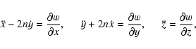
The three-dimensional restricted three-body problem with an oblate primary m₂ is described in a barycentric rotating coordinate system by the equations of motion:

$$\ddot x - 2n\dot y = \frac{\partial w}{\partial x}, \hspace*... ...l y}, \hspace*{0.5cm} \ddot z = \frac{\partial w}{\partial z},$$ (1)

$$w = w_2 = \frac{n^2}{2}\left(x^2+y^2\right)+\frac{1-\mu}{r_1... ... 1+\frac{A_2}{2r_2^2}\left(1-\frac{3z^2}{r_2^2}\right) \right]$$ (2)

(Sharma & Subba Rao 1976; Oberti & Vienne 2003) where:

$$\begin{array}{lll} r_1 &=& \sqrt{(x-\mu)^2+y^2+z^2}, \\ [0.3cm] r_2 &=& \sqrt{(x-\mu+1)^2+y^2+z^2}, \end{array}$$ (3)

are the distances of the massless third body from the primaries, $n=\sqrt{1+3A_2/2}$ is the angular velocity of the rotating coordinate system, and A₂ is the oblateness coefficient of m₂. For values of the mass parameter $\mu = m_2/(m_1+m_2)<1/2$the oblate primary m₂ located on the negative x-axis at $(-1+\mu,0)$ is less massive than m₁, while for $\mu > 1/2$ the primary m₁ located at $(\mu,0)$ is the less massive one. When m₁ is also oblate, with oblateness coefficient A₁, the same equations may be used with w=w₁₂:

 

$$w_{12} =\frac{n^2}{2}\left(x^2+y^2\right)+\frac{1-\mu}{r_1} \left... ...\mu}{r_2} \left[ 1+\frac{A_2}{2r_2^2}\left(1-\frac{3z^2}{r_2^2}\right) \right],$$ (4)

where now $n=\sqrt{1+3(A_1+A_2)/2}$. Finally, when only m₂ is oblate but m₁ is radiating with radiation coefficient q₁, Eq. (1) may be used with w=w₃:

$$w_3 = \frac{n^2}{2}(x^2+y^2)+\frac{q_1(1-\mu)}{r_1}+\frac{\m... ...rac{A_2}{2r_2^2}\left(1-\frac{3z^2}{r_2^2}\right) \right]\cdot$$ (5)

Equations (1) admit the Jacobi integral:

$$2w-(\dot x^2 + \dot y^2 + \dot z^2) = C,$$ (6)

where C is the Jacobi constant.

2 Positions of the out-of-plane equilibrium points

	Figure 1: Position of Lz1(2) in the (x-z) plane as a function of A2 in the interval [0,0.02], for $\mu =0.3$.
Open with DEXTER

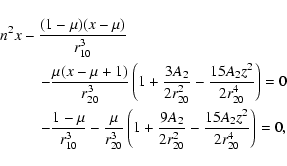
The positions of the out-of-plane equilibrium points can be found from the equations of motion by putting all velocity and acceleration components equal to zero and solving the resulting system, $$\frac{\partial w}{\partial x}=\frac{\partial w}{\partial y}=\frac{\partial w}{\partial z}=0$$, numerically for x, y, z. The second equation is satisfied for y=0, so we must solve the remaining two equations for y=0 and $z\neq 0$. In the case of w₂, for example, we have to solve the system:

$$\begin{array}{ll} &\hspace*{-2.6mm} \displaystyle n^2 x - \fr... ...}{2r_{20}^2}-\frac{15A_2z^2}{2r_{20}^4}\right) = 0, \end{array}$$ (7)

with $r_{10}=\sqrt{(x-\mu)^2+z^2}$, $r_{20}=\sqrt{(x-\mu+1)^2+z^2}$. The out-of-plane equilibrium points are found to be located in the (x-z) plane, above and below the center of each oblate primary in symmetrical positions with respect to the (x-y) plane. In the case of both primaries being oblate the positions of the out-of-plane equilibrium points near m₂, called here L_z1⁽²⁾ and L_z2⁽²⁾, have coordinates $(x_0,0,\pm z_0)$ which can be approximated in the form of power series to third-order terms in A₂ as follows:

$$\begin{array}{lll} x_0 &=& \displaystyle-1+\mu +\frac{9\sqrt{... ...(1-\mu)}{8\mu}A_2^3+{\cal O}\left(A_2^{7/2}\right). \end{array}$$ (8)

By means of the transformation: $\mu \rightarrow 1-\mu$, $A_2 \rightarrow A_1$, $A_1 \rightarrow A_2$, these expansions give the positions of the two equilibrium points above and below m₁, which we call L_z1⁽¹⁾, L_z2⁽¹⁾.

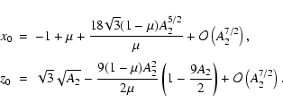
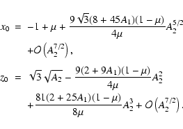
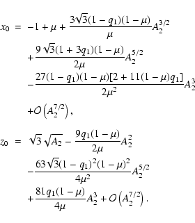
Similarly, in the case of an oblate primary m₂ and a radiating primary m₁ the positions of L_z1⁽²⁾ and L_z2⁽²⁾are approximated to third-order terms in A₂ by:

$$\begin{array}{lll} x_0 &=& \displaystyle-1+\mu+\frac{3\!\sqrt... ...(1-\mu)}{4\mu}A_2^3+{\cal O}\left(A_2^{7/2}\right). \end{array}$$ (9)

In both the above approximations higher order terms can be obtained by solving the relevant equations, e.g. by Newton's method using the software package Mathematica. We note that the use of $x_0=-1+\mu$, $z_0=\sqrt{3}\sqrt{A_2}$, as initial approximations allows the accurate, analytical-approximate or numerical, determination of the position of L_z1⁽²⁾.

In the following we consider the case when only the primary m₂is oblate ($A_2\neq 0$, A₁=0) and the other primary is not radiating (q₁=1). In this case both the above approximations reduce to:

$$\begin{array}{lll} x_0 &=& \displaystyle-1+\mu+\frac{18\!\sq... ...rac{9A_2}{2}\right)+{\cal O}\left(A_2^{7/2}\right). \end{array}$$ (10)

As an example we give in Fig. 1 the position of L_z1⁽²⁾in the (x-z) plane as a function of A₂ in the interval [0,0.02] for $\mu =0.3$, as obtained from (10) (continuous line) and as found numerically (broken line). Note the different scales for the x-axis (horizontal) and the z-axis (vertical). This illustrates that the equilibrium point lies almost exactly above the center of the oblate primary m₂ located at (-0.7,0).

	Figure 2: Zero-velocity curves in the (x-z) plane for $\mu =0.3$ and A2=0.01, 0.015, 0.02, 0.03 ( top to bottom).
Open with DEXTER

3 Zero-velocity curves in the (x - z) plane

Oblateness of primaries and the existence of the out-of-plane equilibrium points has significant effects on the structure of the regions allowed to motion and their boundaries, the zero-velocity surfaces. In this section we present the zero-velocity curves in the (x-z) plane in the case of w₂. As a particular example we show in Fig. 2 the four possible topologies of the curves in this case for $\mu =0.3$. Only the curves for Jacobi constant values corresponding to the collinear equilibrium points and the out-of-plane point L_z1⁽²⁾ (L_z2⁽²⁾) are shown. For clarity, in each case we also show separately (left frame in each row) the curve corresponding to the out-of-plane equilibrium point. These four topologies correspond to four successive intervals of A₂ values, separated by three transition values at which a change of topology occurs. These transitions occur when the Jacobi constant value corresponding to the out-of-plane point coincides with one of the values corresponding to the collinear equilibrium points. In all cases, between the center of the oblate primary and its companion out-of-plane equilibrium points the zero-velocity curves form small ovals of regions not allowed to motion.

4 Stability

To determine the linear stability of the out-of-plane point L_z1⁽²⁾ we transfer the origin to (x₀,0,z₀) and linearize the equations of motion, obtaining:

 

$$\ddot x - 2n\dot y = w_{xx}x+w_{xz}z,$$

$$\ddot y + 2n\dot x = w_{yy}y,$$ (11)

$$\ddot z = w_{zx}x+w_{zz}z,$$

where the partial derivatives are evaluated at the equilibrium point, and w_zx=w_xz. In the present case we also have w_xx+w_yy+w_zz=2n². Stability of L_z1⁽²⁾ is determined by the roots of the characteristic polynomial:

$$\lambda^6 + 2n^2\lambda^4 +\left(w_{xx} w_{yy}+w_{xx}w_{zz}+w_{yy}w_{zz} -w_{xz}^2-4n^2w_{zz}\right) \lambda^2 +w_{yy}(w_{xz}^2-w_{xx}w_{zz}).$$ (12)

We have computed these roots in the case of w₂ for a wide range of $\mu$ and A₂ values and found no case in which the roots are all imaginary. This provides numerical evidence that the out-of-plane equilibrium points are generally unstable.

5 Conclusions

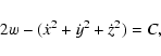
We have found that the equations of motion of the three-dimensional restricted three-body problem with oblateness given in the literature allow the existence of out-of-plane equilibrium points. These points lie in the (x-z) plane almost directly above and below the center of each oblate primary. Their positions are determined numerically and are approximated by series expansions in the oblateness coefficient. Oblateness and the existence of the out-of-plane equilibrium points is seen to have significant effects on the topology of the zero-velocity curves in the (x-z) plane. In particular, between the center of the oblate primary and its companion out-of-plane equilibrium points the zero-velocity curves form small ovals of regions not allowed to motion. Finally, numerical evidence is obtained indicating that these equilibrium points are unstable. We have not checked, however, if their existence might be due to the truncation of the potential employed in deriving the equations of motion.

References

• Gurfil, P., & Meltzer, D. 2005, $25{\rm th}$ Israeli Annual Conference on Aerospace Sciences, preprint (In the text)
• Oberti, P., & Vienne, A. 2003, A&A, 397, 353 [EDP Sciences] [NASA ADS] [CrossRef] (In the text)
• Sharma, R. K. 1987, Ap&SS, 135, 271 [NASA ADS] (In the text)
• Sharma, R. K., & Subba Rao, P. V. 1976, Celes. Mech., 13, 137 [NASA ADS] [CrossRef] (In the text)