A&A 445, 223-232 (2006)
DOI: 10.1051/0004-6361:20053867
On the ionisation fraction in protoplanetary disks
II.
The effect of turbulent mixing on gas-phase chemistry
M. Ilgner - R. P. Nelson
Astronomy Unit, Queen Mary, University of London,
Mile End Road, London E1 4NS, UK
Received 20 July 2005 / Accepted 30 August 2005
Abstract
We calculate the ionisation fraction in protostellar disk
models using two different gas-phase chemical networks, and examine
the effect of turbulent mixing by modelling the diffusion of chemical
species vertically through the disk. The aim is to determine in which
regions of the disk gas can couple to a magnetic field and sustain
MHD turbulence. The disk models are conventional  -disks, and
the primary source of ionisation is X-ray irradiation from the central
star. We assume that the vertical mixing arises because of turbulent
diffusion, and accordingly equate the vertical diffusion coefficient,
-disks, and
the primary source of ionisation is X-ray irradiation from the central
star. We assume that the vertical mixing arises because of turbulent
diffusion, and accordingly equate the vertical diffusion coefficient,
 ,
with the kinematic viscosity,
,
with the kinematic viscosity,  .
.
We find that the effect of diffusion depends crucially on the elemental
abundance of heavy metals (magnesium) included in the chemical model.
In the absence of heavy metals, diffusion has essentially no effect on
the ionisation structure of the disks, as the recombination time scale
is much shorter than the turbulent diffusion time scale. When metals
are included with an elemental abundance above a threshold value, the
diffusion can dramatically reduce the size of the magnetically
decoupled region ("dead zone''), or even remove it altogther. This
arises when recombination is dominated by metal ions, and the
recombination time exceeds the vertical diffusion time scale. For a
complex chemistry the elemental abundance of magnesium required to
remove the dead zone is
 -
10-8. We
also find that diffusion can modify the reaction pathways, giving rise to
dominant species when diffusion is switched on that are minor species when
diffusion is absent. This suggests that there may be chemical signatures
of diffusive mixing that could be used to indirectly detect turbulent
activity in protoplanetary disks.
-
10-8. We
also find that diffusion can modify the reaction pathways, giving rise to
dominant species when diffusion is switched on that are minor species when
diffusion is absent. This suggests that there may be chemical signatures
of diffusive mixing that could be used to indirectly detect turbulent
activity in protoplanetary disks.
We find examples of models in which the dead zone in the outer disk region
is rendered deeper when diffusion is switched on. This is caused by turbulent
mixing diluting the electron fraction in regions where the ionisation degree
is marginally above that required for good coupling.
Overall these results suggest that global MHD turbulence in protoplanetary
disks may be self-sustaining under favourable circumstances, as turbulent
mixing can help maintain the ionisation fraction above that necessary to
ensure good coupling between the gas and magnetic field.
Key words: accretion, accretion disks - magnetohydrodynamics (MHD) - solar system: formation - stars: pre-main sequence
Observational studies of young stars in star forming regions indicate
that protostellar disks are a common occurrence (e.g. Beckwith &
Sargent 1996; Prosser et al. 1994). Many disks show signatures of active
accretion, with the probability of accreting disks being present, and
the appparent gas accretion rate, scaling inversely with the age of the
stellar system in which the young stars are embedded. The canonical value
for the gas accretion rate, however, is often quoted as being

 yr-1 (e.g. Sicilia-Aguilar
et al. 2004).
yr-1 (e.g. Sicilia-Aguilar
et al. 2004).
There are a number of potential mechansims that may lead to angular
momentum transport in protostellar disks, giving rise to the observed mass
accretion. Angular momentum transport that occurs globally throughout the
disk, producing accretion at the observed rates, probably requires turbulence
to act as a source of anomalous viscosity. At the present time the only
source of turbulence in accretion disks that is known to work is the
magnetorotational instability (MRI), which gives rise to MHD turbulence
(Balbus & Hawley 1991; Hawley & Balbus 1991; Hawley et al.
1996).
As has been well documented in the literature, there are continuing
questions about the applicability of the MRI to protostellar disks because
of their high densities and low temperatures that lead to low levels of
ionisation (e.g. Blaes & Balbus 1994; Gammie 1996). Magnetohydrodynamic
simulations of disks including ohmic resistivity (Fleming et al. 2000) show that for magnetic Reynolds numbers
 smaller than
a critical value
smaller than
a critical value
 ,
turbulence cannot be sustained
and the disks return to a near-laminar state. Typically the gas-phase
electron fraction should be
,
turbulence cannot be sustained
and the disks return to a near-laminar state. Typically the gas-phase
electron fraction should be
![$x[{\rm e}_{}^-] \simeq 10_{}^{-12}$](/articles/aa/full/2006/01/aa3867-05/img23.gif) for
disks to be able to sustain MHD turbulence.
for
disks to be able to sustain MHD turbulence.
A number of studies of the ionisation fraction in protostellar disks have
appeared in the literature. Gammie (1996) suggested that disks may have
magnetically "active zones'' sustained by thermal or cosmic ray ionisation,
adjoining regions that were magnetically inactive - "dead zones''. More
recent studies have examined this issue in greater depth. Sano et al. (2000)
used a more complex chemical model that included dust grains. Glassgold et
al. (1997) and Igea et al. (1999) examined the role of X-rays as a source of
ionisation in protoplanetary disks. Fromang et al. (2002) considered the role
of heavy metals in determining the ionisation fraction because of the
potential importance of charge-transfer reactions. Matsumura & Pudritz
(2003) examined the ionisation fraction in the externally heated, passive
disk model proposed by Chiang & Goldreich (1997) using the Sano et al. (2000)
chemical reaction network. Semenov et al. (2004) recently studied disk
chemistry using a complex reaction set drawn from the UMIST database.
In a recent paper (Ilgner & Nelson 2005 - hereafter "Paper I''), we
examined and compared the predictions made by a number of chemical reaction
networks about the ionisation fraction in standard -disk models.
This study included an examination of the reaction scheme proposed by
Oppenheimer & Dalgarno (1974), and more complex schemes drawn from the UMIST
database, in addition to a number of gas-grain chemical networks. In this
paper we extend this initial study to examine the role of turbulent mixing in
determining the ionisation fraction in protoplanetary disk models using gas-phase
chemistry. We consider the simple Oppenheimer & Dalgarno (1974) model, and a
more sophisticated chemical reaction network based on the UMIST database. We
allow the vertical diffusion of each chemical species to occur, equating the
diffusion coefficient
to the kinematic viscosity
that drives
disk accretion. We find that the inclusion of diffusion can have a very
significant effect on the ionisation structure of protoplanetary disks, in
particular when a small abundance of heavy metals (magnesium) is introduced
into the reaction networks. In some cases the disk can modify the ionisation
fraction sufficiently that the dead zone disappears entirely.
This paper is organised as follows. In Sect. 2 we describe the
chemical models, our implementation of the diffusion equation for chemical
species, and the numerical method used to solve the reaction-diffusion equations.
In Sect. 3 we discuss the various models that we compute and present
their results. In Sect. 4 we summarise our main findings and discuss
their potential consequences for protoplanetary disks.
2 Reaction-diffusion model
We consider a system of s chemical species whose local abundances in
the protoplanetary disk evolve due to chemical reactions and vertical
diffusive transport, arising because of concentration gradients and
driven by turbulence. In the discussion below we define r to be the
number of chemical reactions, and n to be the total molar density
(expressed in units of mol cm-3). The global elemental composition
of the system is conserved by applying appropriate boundary conditions
in our reaction-diffusion model.
The underlying disk models considered are standard -disks.
Details are given in Paper I and references therein. To recap: the
disks are assumed to orbit a young solar mass star and undergo viscous
evolution. We use the
prescription for the viscous stress, such
that the kinematic viscosity
 ,
where
,
where  is
the sound speed and
is
the sound speed and  is the local Keplerian angular velocity.
Heating of the disk is provided by viscous dissipation alone, and cooling
by radiation transport in the vertical direction. The disk structure is
obtained by solving for hydrostatic and thermal equilibrium. We employ 30
zones in the vertical direction (from midplane to disk surface) and 100 zones in radius between
is the local Keplerian angular velocity.
Heating of the disk is provided by viscous dissipation alone, and cooling
by radiation transport in the vertical direction. The disk structure is
obtained by solving for hydrostatic and thermal equilibrium. We employ 30
zones in the vertical direction (from midplane to disk surface) and 100 zones in radius between
 AU when computing the chemical
evolution. The underlying disk model was computed using 100 cells in the
vertical direction, and values were interpolated onto the 30 grid points
used in computing the chemistry. The disk models are completely specified
by the mass accretion rate,
AU when computing the chemical
evolution. The underlying disk model was computed using 100 cells in the
vertical direction, and values were interpolated onto the 30 grid points
used in computing the chemistry. The disk models are completely specified
by the mass accretion rate,  and the value of .
We
consider two models: one with
and the value of .
We
consider two models: one with
 yr-1and
 ,
the other with
,
the other with
 yr-1 and
 .
The mass contained in these
models is 0.0087
and 0.0049
respectively. Contour
plots showing the distribution of the kinematic viscosity, ,
are shown
in Figs. 1 and 2.
.
The mass contained in these
models is 0.0087
and 0.0049
respectively. Contour
plots showing the distribution of the kinematic viscosity, ,
are shown
in Figs. 1 and 2.
2.2 Kinetic model
We have applied two different kinetic models for the gas-phase chemistry.
The first is a simple five component model introduced originally by
Oppenheimer & Dalgarno (1974). The second is a much more sophisticated
reaction scheme based on the UMIST database (Le Teuff et al. 2000). We
assume that ionisation of the disk material arises because of incident
X-rays that originate in the corona of the central T Tauri star. We
neglect contributions from Galactic cosmic rays as they are not expected
to penetrate into inner disk regions we consider due to the stellar wind.
The details of these models have been described in Paper I, where they
were given the labels model1 and model3. We maintain
this labelling scheme in this paper so as to establish continuity with
our previous work.
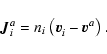
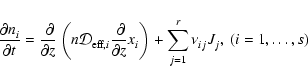
The kinetic equations obey the law of atomic balance:
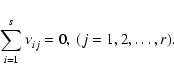 |
(1) |
Here  divided by the molecular mass Mi of the
 component (defined in units of grams/mol) is
proportional to the stoichiometric coefficient, while the
species is involved in the
component (defined in units of grams/mol) is
proportional to the stoichiometric coefficient, while the
species is involved in the
 chemical reaction. The molar density, ni, of the
component is related to the mass density,
chemical reaction. The molar density, ni, of the
component is related to the mass density,
 ,
of the
component through
,
of the
component through
 |
(2) |
The rate of change of the molar density of the
component within a given volume due to chemical reactions and flow of
species i into that volume is
![\begin{figure}
\par\includegraphics[width=8cm,clip]{fig01-ms3867.eps}\end{figure}](/articles/aa/full/2006/01/aa3867-05/Timg41.gif) |
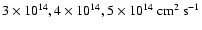
Figure 1:
The kinematic viscosity ;
the contour lines refer to
values
 .
The disk parameters are .
The disk parameters are
 and
and
 . . |
| Open with DEXTER |
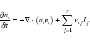 |
(3) |
Jj denotes the chemical reaction rate associated with the
chemical reaction, while
 is the formation/destruction rate of the
component due to the
chemical reaction.
is the formation/destruction rate of the
component due to the
chemical reaction.
 is the velocity of the
component.
is the velocity of the
component.
2.3 Diffusion
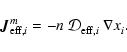
The first term on the right hand side of Eq. (3) represents
the rate of flow of species i into a given volume. In this paper we
assume that the underlying protoplanetary disk is turbulent, and that
turbulent diffusion acts to transport chemical species from one region of
the disk to another. As we are primarily interested in how diffusion affects
the ionisation fraction of the disk material, and we expect the largest
gradients in the electron fraction to be in the vertical (z) direction,
we consider only vertical diffusion in the paper. Equation (3)
becomes
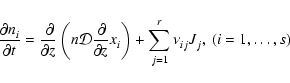 |
(4) |
where
is the turbulent diffusion coefficient, and xi=ni/n
is the fractional abundance of species i. We present a fuller discussion
of the derivation of Eq. (4) in appendix. A similar set of
equations has been used by numerous authors who have examined the effect of
turbulent diffusion on the chemical state of molecular clouds (Xie et al. 1995; Rawlings & Hartquist 1997; Willacy et al. 2002)
and on the role of radial mixing in protoplanetary disks (Wehrstedt & Gail
2002, 2003). In this work we adopt the approximation that
 ,
where
is the kinematic viscosity that drives the radial diffusion of
mass through the protostellar accretion disk. Although there is still some
debate about the precise relationship between the vertical diffusion
coefficient and the effective kinematic viscosity that arises because of MHD
turbulence in astrophysical disks (see Carbillado et al. 2005;
Johansen & Klahr 2005), it is not expected that
,
where
is the kinematic viscosity that drives the radial diffusion of
mass through the protostellar accretion disk. Although there is still some
debate about the precise relationship between the vertical diffusion
coefficient and the effective kinematic viscosity that arises because of MHD
turbulence in astrophysical disks (see Carbillado et al. 2005;
Johansen & Klahr 2005), it is not expected that
 differs
greatly from unity.
differs
greatly from unity.
![\begin{figure}
\par\includegraphics[width=8cm,clip]{fig02-ms3867.eps}\end{figure}](/articles/aa/full/2006/01/aa3867-05/Timg49.gif) |
Figure 2:
The kinematic viscosity ;
the contour lines refer to
values
 .
The disk parameters are .
The disk parameters are
 and
and
 . . |
| Open with DEXTER |
As already discussed, the basic kinetic models that we consider in this
paper are models model1 and model3 described in Paper I.
When these kinetic models are used in conjunction with turbulent mixing
we use the labels model1D and model3D, respectively.
When diffusion is switched off we often use the term "pure kinetic models''
when describing the results in later sections.
2.4 Numerical method
The reaction-diffusion model is governed by the set of s coupled
parabolic partial differential Eq. (4). These equations
can be interpreted as a linear superposition of two operators, one
describing the mass transfer of species i due to diffusion, and the
other describing changes due to chemical reactions. There are a number of
possible approaches to solving these equations. We employed the method
of lines, which is a technique used, e.g., in atmospheric physics that
solves the full system of equations simultaneously (e.g. Chang et al.
1974), rather than a more usual operator splitting approach. Hence, we
transformed the system of s PDEs into a system of
 ODEs,
where nz is the number of grid points in the z direction. Adopting
a uniform mesh along this coordinate direction, we replaced the spatial
derivative in Eq. (4) by a finite differencing scheme.
ODEs,
where nz is the number of grid points in the z direction. Adopting
a uniform mesh along this coordinate direction, we replaced the spatial
derivative in Eq. (4) by a finite differencing scheme.
The boundary conditions are taken to be symmetric at z=0 (disk midplane)
and no flux at z=H (photospheric disk height) for all times t. Applying
the Crank-Nicholsen finite differencing scheme and the chosen boundary
conditions satisfy the conservation of elements and charges at any
cylindrical radius R. Using nz = 30, we found that the elements and
charges are conserved at all cylindrical radii and for all times t. At
 ,
for example, the change in both the elemental
abundances and the total charge was below
10-8 per cent compared
with the corresponding values at
,
for example, the change in both the elemental
abundances and the total charge was below
10-8 per cent compared
with the corresponding values at
 .
.
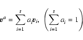
We have allowed all species, including molecular hydrogen and helium, to
be mixed by diffusion. We thus checked a posteriori if the assumed
constancy of the mean molecular weight
 is satisfied. We
find that it is, as expected from the fact that the value of
is satisfied. We
find that it is, as expected from the fact that the value of  is
dominated by hydrogen and helium, and these species do not develop
significant concentration gradients, thus precluding significant diffusion.
is
dominated by hydrogen and helium, and these species do not develop
significant concentration gradients, thus precluding significant diffusion.
We also allowed free electrons to be mixed by diffusion. Differences in the
concentration gradients of the ions and electrons can in principle lead to
different diffusion velocities which may result in a non-zero diffusion flux
of charges per zone. We found, however, that this did not occur.
The reaction-diffusion calculations are initiated with all chemical elements
being in neutral atomic form, apart from hydrogen which is assumed to be in
molecular form. The species were distributed in the disk uniformly. Details are
given in Paper I. Chemical changes lead to concentration gradients that then
initiate the action of diffusion.
3 Results
We have evolved the disk chemistry using the kinetic models described in
Sect. 2.2, including mixing due to turbulent diffusion. The
primary aim of this work is to compare and understand the differences in
the distribution of free electrons that arise in the different models, and
in particular to understand the role that turbulent mixing plays in
determining the free electron fraction and distribution. We wish to determine
which parts of the disk are sufficiently ionised for the gas to be well
coupled to the magnetic field, and thus able to maintain MHD turbulence, and
which regions are too neutral for such turbulence to be maintained. We refer
to those regions as being "active'' and "dead'' zones respectively, with
the region bordering the two being the "transition'' zone. The important
discriminant that determines whether the disk is active or dead is the
magnetic Reynolds number,
,
defined by
 |
(5) |
where H is the disk semi-thickness, cs is the sound speed, and
 is the magnetic diffusivity (not to be confused with the mean molecular
weight). Numerical simulations (e.g. Fleming et al. 2000) indicate
that a critical value of the magnetic Reynolds number,
,
exists such that non linear MHD turbulence cannot be sustained if
falls below
.
We adopt a value of
is the magnetic diffusivity (not to be confused with the mean molecular
weight). Numerical simulations (e.g. Fleming et al. 2000) indicate
that a critical value of the magnetic Reynolds number,
,
exists such that non linear MHD turbulence cannot be sustained if
falls below
.
We adopt a value of
 in this paper, following the value used in
Paper I and Fromang et al. (2002). We are able to calculate the distribution of
within our disks. Regions with
in this paper, following the value used in
Paper I and Fromang et al. (2002). We are able to calculate the distribution of
within our disks. Regions with
 are deemed to
be magnetically dead, and those with
are deemed to
be magnetically dead, and those with
 magnetically active.
When it comes to diffusion we consider the two extremes with the diffusion
coefficient
and
 .
Models with
are labelled model1D and model3D. Models with
reduce to the pure kinetic models model1 and model3 already
discussed in Paper I.
.
Models with
are labelled model1D and model3D. Models with
reduce to the pure kinetic models model1 and model3 already
discussed in Paper I.
We solved the equations by integrating over a time interval of 100 000 yr.
Hence, the ionisation fraction
![$x[{\rm e}^-]$](/articles/aa/full/2006/01/aa3867-05/img60.gif) is a function of time t,
and in principle so is the location of the transition zone. For all kinetic
models, however, the change in the vertical location of the transition zone
at all cylindrical radii in the computational domain was below the grid
resolution for
is a function of time t,
and in principle so is the location of the transition zone. For all kinetic
models, however, the change in the vertical location of the transition zone
at all cylindrical radii in the computational domain was below the grid
resolution for
 .
.
3.1 Diffusion versus recombination
In order for diffusion to modify the ionisation fraction of material near
the transition zone in protoplanetary disks, and hence modify the size of
the dead zone, the vertical diffusion time should be less than the
recombination time for free electrons.
We consider diffusion across a scale height at
 AU in the
heavier disk model. The scale height of this disk is given by
AU in the
heavier disk model. The scale height of this disk is given by
 (see Paper I). Figure 1 shows
that the kinematic viscosity at 5 AU is
(see Paper I). Figure 1 shows
that the kinematic viscosity at 5 AU is
 cm2
s-1, which we adopt as the value for the vertical diffusion coefficient
.
The diffusion time is given by
cm2
s-1, which we adopt as the value for the vertical diffusion coefficient
.
The diffusion time is given by
 |
(6) |
We consider a simple chemistry (described in detail in
Sect. 3.2) involving a representative molecule and its ion,
"m'' and "m+'', and a representative heavy metal and its ion, "M''
and "M+''. In regions well shielded from X-rays, the recombination
rate of free electrons is given by
![\begin{displaymath}\frac{{\rm d} x[{\rm e}_{}^-]}{{\rm d}t} = - k_1^{} x[{\rm e}...
...{}}]
- k_2^{} x[{\rm e}_{}^-] x[{\rm M}_{}^+] N[{\rm H_2^{}}]
\end{displaymath}](/articles/aa/full/2006/01/aa3867-05/img66.gif) |
(7) |
where k1 is the rate coefficient for recombination between molecular
ions and electrons, k2 is the equivalent for heavy metal ions, and
![$N[{\rm H_2^{}}]$](/articles/aa/full/2006/01/aa3867-05/img67.gif) is the number density of hydrogen molecules. The two
scenarios of interest are the metal-free case and the metal-dominated
case.
is the number density of hydrogen molecules. The two
scenarios of interest are the metal-free case and the metal-dominated
case.
In the metal-free case, where the electron fraction
![$x[{\rm e}_{}^-] = x[{\rm m_{}^+}]$](/articles/aa/full/2006/01/aa3867-05/img68.gif) ,
Eq. (7) becomes
,
Eq. (7) becomes
![\begin{displaymath}\frac{{\rm d} x[{\rm e}_{}^-]}{{\rm d}t} = - k_1 x^2[{\rm e}_{}^-] N[{\rm H_2^{}}].
\end{displaymath}](/articles/aa/full/2006/01/aa3867-05/img69.gif) |
(8) |
Assuming
remains constant, Eq. (8)
integrates to give the recombination time
![\begin{displaymath}\tau_{\tilde{\alpha}} = \frac{1}{k_1 N[{\rm H_2}]} \left[\frac{1}{x_{{\rm e}^-}^f} -
\frac{1}{x_{{\rm e}^-}^i}\right],
\end{displaymath}](/articles/aa/full/2006/01/aa3867-05/img70.gif) |
(9) |
where
 and
and
 are the initial and final values of
 during diffusion over a scale height. At R=5 AU, the electron
abundance at the transition zone is
during diffusion over a scale height. At R=5 AU, the electron
abundance at the transition zone is
 ,
as shown
in Fig. 7 of Paper I. The rate coefficient
,
as shown
in Fig. 7 of Paper I. The rate coefficient
 ,
,
![$N[{\rm H}_2^{}] \simeq 5 \times 10^{12}$](/articles/aa/full/2006/01/aa3867-05/img76.gif) cm-3, and
cm-3, and
 K (see Figs. 1 and 2 in Paper I). The recombination time is
then
K (see Figs. 1 and 2 in Paper I). The recombination time is
then
 days. It is clear that diffusion is
not expected to have a significant impact on the dead zone structure in this
case.
days. It is clear that diffusion is
not expected to have a significant impact on the dead zone structure in this
case.
The rate coefficient appropriate to the metal-dominated case is
 ,
which gives a recombination time of
,
which gives a recombination time of
 4200 yr. Comparing this with the diffusion time
 yr, it is clear that a protoplanetary disk with a
significant population of gas-phase heavy metals should have the structure
of the dead zone modified substantially by the action of turbulent diffusion.
yr, it is clear that a protoplanetary disk with a
significant population of gas-phase heavy metals should have the structure
of the dead zone modified substantially by the action of turbulent diffusion.
3.2 Oppenheimer & Dalgarno model
The underlying kinetic model of model1D involves two elements,
five species/components, and four reactions. These species are free
electrons "e-'', a representative molecule "m'', a heavy metal
atom "M'', and their ionized counterparts "m+'' and "M+''.
The rate coefficients for the ionisation of m and for dissociative
Table 1:
Rate coefficients applied for the Oppenheimer &
Dalgarno model. The values are always used as reference values.
recomination of m+ are given by  and
and
 ,
while
the rate coefficients
,
while
the rate coefficients
 and
and
 apply to the
charge-transfer reaction between m+ and M and the radiative
recombination of M+, respectively. The rate coefficients are listed
in Table 1 and were used in all model1D
calculations unless stated otherwise. Results obtained in Paper I showed
that the dead zones obtained using model1 were always smaller
than those obtained for the complex models. We find it useful, however,
to analyse model1 and model1D as many of the features
of this simple model can be helpful in understanding the more complex
model.
apply to the
charge-transfer reaction between m+ and M and the radiative
recombination of M+, respectively. The rate coefficients are listed
in Table 1 and were used in all model1D
calculations unless stated otherwise. Results obtained in Paper I showed
that the dead zones obtained using model1 were always smaller
than those obtained for the complex models. We find it useful, however,
to analyse model1 and model1D as many of the features
of this simple model can be helpful in understanding the more complex
model.
The results obtained for model1D are presented in
Fig. 3, which shows the column density of the whole
disk plotted as a function of radius using the solid line, and the column
density of the active zone only using either dotted lines (for which
)
or dashed lines (for which
).
The first thing to note is that diffusive mixing makes essentially no
difference to the size of the active zone when heavy metals are not
included in the chemistry. This is illustrated by the lowest line plotted
in Fig. 3, which appears as a dash-dotted line in the
figure, but is actually a dashed line (representing the case with diffusion
![\begin{figure}
\par\includegraphics[width=8cm,clip]{fig03-ms3867.eps}\end{figure}](/articles/aa/full/2006/01/aa3867-05/Timg93.gif) |
Figure 3:
model1(D) - Column densities of the whole disk
(solid line) and of the active zones (dashed and dotted lines) -
refering to magnetic Reynolds numbers greater than 100 - for
different values
 .
While the
dashed lines refer to simulations with
,
the dotted lines refer to simulations with
.
The reference values for the rate coefficients are applied. The disk
parameters are
and .
While the
dashed lines refer to simulations with
,
the dotted lines refer to simulations with
.
The reference values for the rate coefficients are applied. The disk
parameters are
and
 . . |
| Open with DEXTER |
switched on) plotted over a dotted line (representing the case when diffusion
is switched off). The reason for this result is simple: the recombination
time when metals are absent is very much shorter than the turbulent mixing
time. As a parcel of fluid moves from the active region of the disk toward
the dead zone, free electrons will recombine with molecular ions rapidly,
making no change to the ionisation fraction of the dead region.
Increasing the heavy metal elemental abundance from zero to
 and switching diffusion on also makes no difference
to the size of the dead zone. The addition of such a small fraction of metals
does not prevent recombination between molecular ions and electrons being
the dominant destruction process of the free electrons. This is illustrated by
the second lowest line in Fig. 3.
and switching diffusion on also makes no difference
to the size of the dead zone. The addition of such a small fraction of metals
does not prevent recombination between molecular ions and electrons being
the dominant destruction process of the free electrons. This is illustrated by
the second lowest line in Fig. 3.
Increasing the heavy metal fraction to
 results in a
significant change in the structure of the dead zone when diffusion is
switched on. Interior to
results in a
significant change in the structure of the dead zone when diffusion is
switched on. Interior to  AU there is almost no change in the size
of the active zone because recombination between electrons and molecular ions
is still the dominant process determining the ionisation fraction. Beyond
AU there is almost no change in the size
of the active zone because recombination between electrons and molecular ions
is still the dominant process determining the ionisation fraction. Beyond
 AU, however, the dead zone disappears completely when diffusion is
switched on, whereas as a dead zone remains when
AU, however, the dead zone disappears completely when diffusion is
switched on, whereas as a dead zone remains when
 and
.
The reason for this difference is simple. The charge-transfer
reaction between molecular ions and neutral heavy metals removes most of the
molecular ions beyond AU. This allows the recombination between metal
ions and electrons to become the primary means by which free electrons are
destroyed. The recombination time for this reaction, however, is much longer
than for recombination between molecular ions and electrons, and is also longer
than the turbulent mixing time. As a parcel of fluid moves from the active zone
toward the dead zone, the time it takes is shorter than the time scale over which
the free electrons are destroyed, thus increasing the free electron fraction in
the dead zone and allowing it to become active.
and
.
The reason for this difference is simple. The charge-transfer
reaction between molecular ions and neutral heavy metals removes most of the
molecular ions beyond AU. This allows the recombination between metal
ions and electrons to become the primary means by which free electrons are
destroyed. The recombination time for this reaction, however, is much longer
than for recombination between molecular ions and electrons, and is also longer
than the turbulent mixing time. As a parcel of fluid moves from the active zone
toward the dead zone, the time it takes is shorter than the time scale over which
the free electrons are destroyed, thus increasing the free electron fraction in
the dead zone and allowing it to become active.
In order to explore further the role played by the relative diffusion and
recombination time scales, and to examine conditions under which the
reaction-diffusion model deviates from the pure kinetic model, we have
performed some numerical experiments in which we have artificially modified
recombination times. We discuss these briefly below.
Case:

In this case, model1D reduces to a three component system with two
reactions. The molecular ion m+ and the free electron  are formed and
destroyed by the same chemical reaction. Since m+ and
are formed and
destroyed by the same chemical reaction. Since m+ and
 are mixed
with the same diffusion velocity, it is simple to demonstrate how the mixing
time scale,
are mixed
with the same diffusion velocity, it is simple to demonstrate how the mixing
time scale,
 ,
and the molecular ion-electron recombination
time scale,
,
and the molecular ion-electron recombination
time scale,
 ,
affect the ionisation fraction
,
affect the ionisation fraction
![$x[{\rm e}^-_{}]$](/articles/aa/full/2006/01/aa3867-05/img104.gif) (where
(where
 and
and
 ). We systematically changed
the ratio
). We systematically changed
the ratio
 by changing the rate coefficient
of the molecular ion-electron recombination reaction. We
find that the recombination time scale
has to be
increased by three orders of magnitude before the results of the
reaction-diffusion model model1D deviates from the pure kinetic
model model1. This illustrates the basic point that reasonable
diffusion rates will be unable to change the size of the dead zone obtained
using the Oppenheimer & Dalgarno model in the absence of heavy metals in
the gas phase.
by changing the rate coefficient
of the molecular ion-electron recombination reaction. We
find that the recombination time scale
has to be
increased by three orders of magnitude before the results of the
reaction-diffusion model model1D deviates from the pure kinetic
model model1. This illustrates the basic point that reasonable
diffusion rates will be unable to change the size of the dead zone obtained
using the Oppenheimer & Dalgarno model in the absence of heavy metals in
the gas phase.
Case:

We performed a similar exercise to that just described, but included heavy
metals with an elemental concentration of
 .
This value causes the recombination of metal ions with free electrons to
dominate over recombination with molecular ions beyond
AU. We used
the reference values for the rate coefficients
and
listed in Table 1, and modified
systematically the recombination rate coefficient
between
metals and electrons only.
.
This value causes the recombination of metal ions with free electrons to
dominate over recombination with molecular ions beyond
AU. We used
the reference values for the rate coefficients
and
listed in Table 1, and modified
systematically the recombination rate coefficient
between
metals and electrons only.
 now becomes the dominant recombination time scale. Figure 3
shows that the addition of metals with
now becomes the dominant recombination time scale. Figure 3
shows that the addition of metals with
 causes
a substantial difference between the reaction-diffusion model and the pure
kinetic model. We find that we need to decrease the value of
causes
a substantial difference between the reaction-diffusion model and the pure
kinetic model. We find that we need to decrease the value of
 by two orders of magnitude in order that diffusion has
no impact on the size of the dead zone.
by two orders of magnitude in order that diffusion has
no impact on the size of the dead zone.
One can consider this issue in reverse, and ask what changes need to be made
to
in the pure kinetic model model1 in order
for it to give the same sized dead zone as model1D with
and the standard value of
.
We find that if
is increased by two orders of magnitude in
model1 then the resulting dead zone is the same as obtained in the
standard model1D. For this particular reaction network, this indicates
that diffusion acts as an effective reduction in the dominant recombination
rate coefficient.
The underlying kinetic model in model3D was constructed by
extracting all species and reactions from a given species set of 174 species
and the UMIST database containing the elements H, He, C, O, N, S, Si, Mg, Fe.
1965 reactions were extracted from the UMIST database. A full description is
given in Paper I. Compared with the previous model of Oppenheimer & Dalgarno
(model1D) there are now many pathways through which free electrons
can recombine with molecular ions, each with their own associated time scale.
Without knowing a priori which ion is dominant, it is difficult to make
estimates of the relative mixing and recombination time scales. Indeed, our
previous study presented in Paper I suggests that there is more than one
dominant ion that determines the ionisation fraction, complicating the picture
further.
An additional complication is that the introduction of diffusion into the kinetic
model can modify the chemical pathways, such that comparing the products of the
pure kinetic models with those of the reaction-diffusion models becomes difficult.
This effect manifests itself in our study by changing the identities of the molecular
ions which are dominant in the transition region between dead and active zones.
We now discuss the results obtained using model3D, beginning with models
for which the heavy metal, magnesium, was neglected from the chemical network,
before discussing the effects that including Mg has on the ionisation fraction and
resulting dead zone structure.
Case:

We begin by discussing the results of model3D
![\begin{figure}
\par\includegraphics[width=8cm,clip]{fig04-ms3867.eps}\end{figure}](/articles/aa/full/2006/01/aa3867-05/Timg113.gif) |
Figure 4:
model3(D) - Column densities of the whole disk
(solid line) and of the active zones (dashed and dotted lines) -
refering to magnetic Reynolds numbers greater than 100 - for
.
While the dashed line refers to
simulations with
,
the dotted line
refers to simulation with
.
The disk
parameters are
and
. |
| Open with DEXTER |
applied to the disk model defined by
and
before
discussing the results obtained in the disk model with
and
 .
As a general result we find that the location of the transition zone
(which separates the active and the dead zones) is very similiar when
comparing the results obtained for both disk models by applying a
reaction-diffusion model with
and
,
respectively. This is illustrated by Fig. 4
in which the column density of the whole disk is plotted using the
solid line, the column density of the active zone obtained using the
pure kinetic model is plotted using the dotted line, and the results
of the reaction-diffusion model are plotted using the dashed line. We
see that model3D with
produces a slightly
larger active zone within
.
As a general result we find that the location of the transition zone
(which separates the active and the dead zones) is very similiar when
comparing the results obtained for both disk models by applying a
reaction-diffusion model with
and
,
respectively. This is illustrated by Fig. 4
in which the column density of the whole disk is plotted using the
solid line, the column density of the active zone obtained using the
pure kinetic model is plotted using the dotted line, and the results
of the reaction-diffusion model are plotted using the dashed line. We
see that model3D with
produces a slightly
larger active zone within
 ,
but beyond
this region the depth of the active zone is unaffected by diffusive
mixing.
,
but beyond
this region the depth of the active zone is unaffected by diffusive
mixing.
We have examined the abundances of the key molecular ions in the
transition region between the active and dead zones. Typically the
ionisation balance is not determined by a single dominant ion, but
by a small number of ions. We find clear differences between the pure
kinetic model and the reaction-diffusion model in those regions in
radius where there is the greatest difference in the depth of the active
zone between the two models.
HCNH+ and NH4+ are the most abundant ions in the neighbourhood
of the transition zone between
 obtained for
the pure kinetic model. It is important to note that the ratio between
both ion concentrations does not change gradually in the vicinity of the
transition zone, but instead there is a sharp transition: above the
transition zone HCNH+ is more abundant than NH4+ by one order
of magnitude. This ratio becomes inverted just below the transition zone
by the same order of magnitude. Due to the significantly shorter
recombination time scale, electrons recombine more efficiently with NH4+
than with HCNH+. Hence, NH4+ determines the location of the
transition zone rather than HCNH+.
obtained for
the pure kinetic model. It is important to note that the ratio between
both ion concentrations does not change gradually in the vicinity of the
transition zone, but instead there is a sharp transition: above the
transition zone HCNH+ is more abundant than NH4+ by one order
of magnitude. This ratio becomes inverted just below the transition zone
by the same order of magnitude. Due to the significantly shorter
recombination time scale, electrons recombine more efficiently with NH4+
than with HCNH+. Hence, NH4+ determines the location of the
transition zone rather than HCNH+.
By contrast, the abundance of NH4+ is significantly lowered by applying
the reaction-diffusion model with
.
Now, the more complex ion
 is two orders of magnitude more abundant
than the next most abundant ion
is two orders of magnitude more abundant
than the next most abundant ion
 .
In addition, since
mixing tends to reduce the concentration gradients of each species with height,
z, the ratio between both ion concentrations
.
In addition, since
mixing tends to reduce the concentration gradients of each species with height,
z, the ratio between both ion concentrations
![$x[{\rm H_4^{}C_2^{}N_{}^+}]/x[{\rm CH_3^{}OH_2^+}]$](/articles/aa/full/2006/01/aa3867-05/img119.gif) changes gradually
when passing through the transition zone. In the same region between
changes gradually
when passing through the transition zone. In the same region between
 we found significant differences in the distribution
of most of the species obtained for a reaction-diffusion model and the
corresponding pure kinetic model. This is a clear indication that mixing may
change the kinetics significantly.
we found significant differences in the distribution
of most of the species obtained for a reaction-diffusion model and the
corresponding pure kinetic model. This is a clear indication that mixing may
change the kinetics significantly.
We now consider the
,
 disk model. The results
for this model are shown in Fig. 5. We first note
that this disk model generates an intrinisically deeper dead zone in the outer
regions of the disk beyond
disk model. The results
for this model are shown in Fig. 5. We first note
that this disk model generates an intrinisically deeper dead zone in the outer
regions of the disk beyond  AU, even though the ionisation rate due
![\begin{figure}
\par\includegraphics[width=8cm,clip]{fig05-ms3867.eps}\end{figure}](/articles/aa/full/2006/01/aa3867-05/Timg123.gif) |
Figure 5:
model3(D) - Column densities of the whole disk
(solid line) and of the active zones (dashed and dotted lines) -
refering to magnetic Reynolds numbers greater than 100 - for
.
While the dashed line refers to
simulation with
,
the dotted line
refers to simulation with
.
The disk
parameters are
and
. |
| Open with DEXTER |
to X-rays is higher due to the smaller surface density. This is a temperature
effect that arises because the viscous heating is reduced because of the smaller
and
values. The recombination rates scale according to
 ,
leading to a lower ionisation fraction.
,
leading to a lower ionisation fraction.
We focus in particular on locations
 where the
most significant differences in the vertical depth of the active zone appear
when comparing the reaction-diffusion model and the corresponding pure kinetic
model.
where the
most significant differences in the vertical depth of the active zone appear
when comparing the reaction-diffusion model and the corresponding pure kinetic
model.
The most abundant ions produced by the pure kinetic model in the neighbourhood
of the transition zone are
and NH4+. These
species are similarly abundant, but the recombination time for electrons with
NH4+ is much shorter than with
,
so NH4+
determines the position of the transition zone. The corresponding
reaction-diffusion model again results in
![$x[{\rm NH_4^+}]$](/articles/aa/full/2006/01/aa3867-05/img126.gif) dropping
significantly so that it no longer controls the ionisation fraction in the
neighbourhood of the transition zone. Instead,
is
the most abundant molecular ion, being one order of magnitude more abundant than
the next most abundant ion
dropping
significantly so that it no longer controls the ionisation fraction in the
neighbourhood of the transition zone. Instead,
is
the most abundant molecular ion, being one order of magnitude more abundant than
the next most abundant ion
 .
This is again evidence that
the presence of turbulent mixing in a protoplanetary disk can change the reaction
kinetics. This leads to the intriguing possibility that such changes may in the
future act as observational diagnostics for the presence of turbulence in disks.
.
This is again evidence that
the presence of turbulent mixing in a protoplanetary disk can change the reaction
kinetics. This leads to the intriguing possibility that such changes may in the
future act as observational diagnostics for the presence of turbulence in disks.
Case:

We now consider the effect that including magnesium has on the models. We begin
by discussing the results obtained for
![\begin{figure}
\par\includegraphics[width=8cm,clip]{fig06-ms3867.eps}\end{figure}](/articles/aa/full/2006/01/aa3867-05/Timg129.gif) |
Figure 6:
model3(D) - Column densities of the whole disk
(solid line) and of the active zones (dashed and dotted lines) -
refering to magnetic Reynolds numbers greater than 100 - for
different values of
 .
While the dashed lines
refer to simulations with
,
the dotted
lines refer to simulations with
.
Especially, for a reaction-diffusion model with .
While the dashed lines
refer to simulations with
,
the dotted
lines refer to simulations with
.
Especially, for a reaction-diffusion model with
 no dead zones are observed above
values
no dead zones are observed above
values
 .
The disk parameters are
and
. .
The disk parameters are
and
. |
| Open with DEXTER |
the disk model with
,
 .
The results for
model3D are shown in Fig. 6. The
dotted lines show the column density of the active zones obtained by
the pure kinetic model for various values of
.
The results for
model3D are shown in Fig. 6. The
dotted lines show the column density of the active zones obtained by
the pure kinetic model for various values of
 .
The dashed
lines show the column density of the active zones obtained by the
reaction-diffusion model. In general we find that mixing affects the
size of the active zone significantly as soon as metals with
concentrations above a threshold value are involved.
.
The dashed
lines show the column density of the active zones obtained by the
reaction-diffusion model. In general we find that mixing affects the
size of the active zone significantly as soon as metals with
concentrations above a threshold value are involved.
The addition of magnesium with elemental concentration
 makes very little difference to the size
of the dead zone, whether diffusion is switched on or not, as seen by
comparing Figs. 4 and
6. This is because a low value of
does not allow
makes very little difference to the size
of the dead zone, whether diffusion is switched on or not, as seen by
comparing Figs. 4 and
6. This is because a low value of
does not allow
 to become the dominant
ion via charge-transfer reactions.
to become the dominant
ion via charge-transfer reactions.
Increasing the magnesium elemental abundance to
 changes the picture dramatically when
diffusion is switched on. The pure kinetic models with these magnesium
abundances included contain no regions in the disk beyond
changes the picture dramatically when
diffusion is switched on. The pure kinetic models with these magnesium
abundances included contain no regions in the disk beyond  AU
where the disk is fully active, although the dead zone tends to shrink
beyond
AU. In this region
followed by
AU
where the disk is fully active, although the dead zone tends to shrink
beyond
AU. In this region
followed by
 are the most dominant ions, while in the region
 AU the
 ion is dominant. The reaction-diffusion model model3D
with
and
ion is dominant. The reaction-diffusion model model3D
with
and
 produces a dead zone of
similar depth to the pure kinetic model between radii
AU.
The identity of the dominant molecular ion in this region changes, however,
when diffusion is switched on. The abundances of
and
are found to decrease significantly, and are replaced by the
ion
produces a dead zone of
similar depth to the pure kinetic model between radii
AU.
The identity of the dominant molecular ion in this region changes, however,
when diffusion is switched on. The abundances of
and
are found to decrease significantly, and are replaced by the
ion
 .
The disk is rendered fully active beyond
AU
where
is the dominant ion and the recombination time increases
above the mixing time.
.
The disk is rendered fully active beyond
AU
where
is the dominant ion and the recombination time increases
above the mixing time.
model3D with
and
 produces
a fully active disk, in contrast to the corresponding pure kinetic model
model3. For these higher magnesium abundances,
produces
a fully active disk, in contrast to the corresponding pure kinetic model
model3. For these higher magnesium abundances,
 becomes
the dominant ion through the charge-transfer reaction with molecular ions, and
the abundance of
is much reduced. The long electron recombination
time associated with
allows diffusive mixing to maintain a disk
that is fully active.
becomes
the dominant ion through the charge-transfer reaction with molecular ions, and
the abundance of
is much reduced. The long electron recombination
time associated with
allows diffusive mixing to maintain a disk
that is fully active.
We now consider the disk model with
,
 .
The results are presented in
Fig. 7, where the column density of the active
zones obtained using the pure kinetic models are plotted using dotted lines.
Dashed lines represent the column density of active zones obtained using the
reaction-diffusion model.
.
The results are presented in
Fig. 7, where the column density of the active
zones obtained using the pure kinetic models are plotted using dotted lines.
Dashed lines represent the column density of active zones obtained using the
reaction-diffusion model.
Adding magnesium with an elemental abundance
 results
in very little change in the size of the dead zone whether diffusion is switched
on or not (compare Figs. 5 and 7).
results
in very little change in the size of the dead zone whether diffusion is switched
on or not (compare Figs. 5 and 7).
Increasing the magnesium elemental concentration to
causes substantial changes to occur when diffusion is switched on. Interior to
 AU there is no change because the molecular ions
and
are dominant over
there, both with and without
diffusive mixing. Between
AU there is no change because the molecular ions
and
are dominant over
there, both with and without
diffusive mixing. Between
 AU the disk becomes fully active
when diffusion is switched on, but maintains a significant dead zone there in
the pure kinetic model. The influence of
allows the recombination
time to be increased so that mixing can render the disk active. Beyond
AU the disk becomes fully active
when diffusion is switched on, but maintains a significant dead zone there in
the pure kinetic model. The influence of
allows the recombination
time to be increased so that mixing can render the disk active. Beyond  AU we obtain the surprising result that diffusive mixing causes the depth of the
![\begin{figure}
\par\includegraphics[width=8cm,clip]{fig07-ms3867.eps}\end{figure}](/articles/aa/full/2006/01/aa3867-05/Timg148.gif) |
Figure 7:
model3(D) - Column densities of the whole disk
(solid line) and of the active zones (dashed and dotted lines) -
refering to magnetic Reynolds numbers greater than 100 - for
different values of
.
While the dashed lines
refer to simulations with
,
the
dotted lines refer to simulations with
.
The disk parameters are
and
. |
| Open with DEXTER |
dead zone to increase rather than decrease. The reason for this is that the
ionisation fraction at large radii in the pure kinetic model is always close to
the critical value for the disk to be active. The addition of diffusion appears
to have a diluting effect on the electron fraction in the active zone, which
causes the dead zone to increase in size.
Increasing the magnesium elemental concentration to
 causes
further changes to occur when diffusion is switched on. The
ion is
dominant throughout the disk, and the disk model is rendered entirely active
between the radii
causes
further changes to occur when diffusion is switched on. The
ion is
dominant throughout the disk, and the disk model is rendered entirely active
between the radii
 AU. We again find that the dead zone becomes
deeper at radii beyond
AU. We again find that the dead zone becomes
deeper at radii beyond  AU when diffusive mixing is effective. The reason
is the same as given above: the ionisation fraction at these radii is always close
to the critical value required to render the disk active. Diffusive mixing dilutes
the electron fraction there, producing a deeper dead zone.
AU when diffusive mixing is effective. The reason
is the same as given above: the ionisation fraction at these radii is always close
to the critical value required to render the disk active. Diffusive mixing dilutes
the electron fraction there, producing a deeper dead zone.
4 Summary
We have presented the results of calculations that examine the ionisation fraction
in protoplanetary disks models. Our models compute the chemical evolution of the gas,
with X-rays from the central star being the primary source of ionisation, and also
include vertical diffusion of the chemical species. This diffusion is designed to
mimic the effects of turbulent mixing arising from the MHD turbulence that is thought
to drive accretion in protostellar disks (e.g. Balbus & Hawley 1991).
The main findings of this work are:
- The simple Oppenheimer & Dalgarno (1974) kinetic model produces smaller
dead zones than a more complete kinetic model based on the UMIST database. This
is true whether diffusion is switched on or not.
- All models which did not include heavy metals (magnesium) give rise to
substantial dead zones. The inclusion of diffusion in these cases makes very
little difference to the size and depth of the dead zone. This is because the
recombination of molecular ions with electrons occurs too rapidly for turbulent
mixing to be effective.
- The addition of heavy metals (magnesium) to the reaction networks can
give rise to dramatic changes in the sizes of dead zones when diffusion is
included. This is because the recombination time between metal ions and
electrons is orders of magnitudes longer than that between molecular ions and
electrons, and is longer than the diffusive mixing time. The addition of metals,
combined with charge-transfer reactions, removes most of the molecular ions and
replaces them with the longer lived metal ions.
- For the Oppenheimer & Dalgarno (1974) network, the addition of heavy metals
with fractional abundance
leads to the dead zone
disappearing beyond
AU when diffusion is switched on. In the absence of
diffusion a substantial dead zone exists in this region of this disk.
- For the model based on the UMIST database, the addition of magnesium to the
chemical network with a fractional abundance of
leads to
the dead zone disappearing beyond
AU when diffusion is switched on. When
the abundance of magnesium is increased to
the dead zone
disappears completely. Models in which diffusion is not present, but with the same
magnesium abundances have substantial dead zones.
- We find that the changes in the size of dead zones when diffusion is switched
on do not only arise because free electrons are mixed into the dead zone, but also
because the chemical pathways are modified by diffusion. One effect of this in our
models is that the dominant ions near the transition zone between dead and active
zones change their identity when diffusion is initiated. This raises the interesting
possibility that there may be chemical signatures of turbulent diffusion that can
act potentially as observational diagnostics of turbulence in protoplanetary disks.
- For some disk models, the inclusion of diffusion can cause the dead zone
depth to increase in the outer regions of the disk. This arises because these
particlar models predict that the electron fraction is only slightly above the
critical value for the disk to be active in these regions when diffusion is switched
off. Switching diffusion on can dilute the electron fraction in these regions,
leading to a deeper dead zone.
Overall, our models indicate that turbulence in protoplanetary disks can be a
self-sustaining process, providing that certain criteria are met, and indicate
that dead zones can be reduced or removed altogther through turbulent mixing
processes. These criteria are:
- (i)
- There are sufficient magnesium atoms available in the gas phase so that recombination
between magnesium ions and electrons becomes the dominant process by which the local
ionisation fraction is determined.
- (ii)
- The turbulent diffusion time scale is shorter than the dominant recombination
time on which free electrons are removed.
A potentially serious omission from our models is the existence of small dust grains.
These are known to sweep up free electrons (and metal atoms) very efficiently, and
when included with the interstellar abundance they substantially increase the size and
depth of dead zones in protoplanetary disks (see Sano et al. 2000; Paper I). It is very
likely that these grains will need to be substantially depleted by grain growth before
the effects of turbulent mixing described in this paper are realised, as the removal
rate of electrons from the gas phase is too large to allow diffusion to be effective.
An interesting question is whether a disk that has a substantial dead zone, and which
is subject to a temporary period of intense ionisation (by large X-ray flares of the
type recently report by Feigelson et al. 2005, for example), can enter into a
self-sustaining turbulent state in which the turbulent mixing maintains a fully active
disk. This question is currently under investigation and will be the subject of a future
publication. An equally interesting question is whether a disk with a substantial dead
zone, sandwiched between active zones near the disk surface, can become globally active
due to turbulent motions overshooting into the dead zone and transporting free electrons
into it. This question cannot be addressed by calculations of the type presented in this
paper, but their results suggest that this may be possible under certain circumstances.
Acknowledgements
This research was supported by the European Community's Research
Training Networks Programme under contract HPRN-CT-2002-00308,
"PLANETS''.
Appendix
The diffusion flow
 of the
component may be expressed in various ways depending which
reference velocity
of the
component may be expressed in various ways depending which
reference velocity
 is used. The molar diffusion
flow
is
is used. The molar diffusion
flow
is
 |
(A.1) |
The reference velocities
 are defined as weighted
averages of the velocity
of the
component
are defined as weighted
averages of the velocity
of the
component
 |
(A.2) |
with ai as normalised weights.
Since the mass is conserved, the diffusion fluxes of the
s components are not independent. Specifying the reference
velocity
by the mean molar velocity

 |
(A.3) |
where xi denotes the molar fraction of the
component
 |
(A.4) |
the molar diffusion fluxes are constrained by
 |
(A.5) |
There are several contributions to the diffusion flux. We assume
that the most important contribution to the diffusion flux is
caused by concentration gradients rather than due to pressure
gradients, external forces, and coupled effects (cross-effects).
Diffusion caused by concentration gradients is called
"ordinary" diffusion. Considering ordinary diffusion processes
only, we often use the phrase "diffusion" instead of "ordinary"
diffusion. The (ordinary) diffusion is described by the
phenomenological equation, which is well-known as Fick's first
law for a binary system s = 2. By analogy to the molar diffusion
flow for a binary system, we define an effective molar diffusion
flow
 for the diffusion of the
ith component in a mixture by
for the diffusion of the
ith component in a mixture by
 |
(A.6) |
The effective binary diffusivity
 for species i in a mixture can be calculated from the diffusivity
 of the pair i-j in a binary mixture by applying
the so-called "Stefan-Maxwell equation''. Especially, for systems
in which all the
are the same
is now given by
of the pair i-j in a binary mixture by applying
the so-called "Stefan-Maxwell equation''. Especially, for systems
in which all the
are the same
is now given by
 |
(A.7) |
Because of the definition of the molar diffusion flow
,
see Eq. (A.1), the velocity of the
component and the reference velocity
are related to
eachother. In particular, in a molar diluted system![[*]](/icons/foot_motif.gif) we deal with,
one can approximate the reference velocity by
we deal with,
one can approximate the reference velocity by
 .
Similiar applies for mass diluted
systems with
.
Similiar applies for mass diluted
systems with
 where
where
 denotes
the
denotes
the
 component velocity. This is in agreement
with the hydrostatic equilibrium assumption in z direction. Finally,
Eq. (3) can be simplified by:
component velocity. This is in agreement
with the hydrostatic equilibrium assumption in z direction. Finally,
Eq. (3) can be simplified by:
 |
(A.8) |
constraint by Eq. (A.5). Note that we simplified the
symbol for the effective binary diffusivity for species i in a mixture
by using
instead of
.
Because of the molar diluted system we consider and due to the fact
that the most abundant components (which are molecular hydrogen and
helium) do not contribute to the molar diffusion fluxes, the
mass is conserved even by neglecting Eq. (A.5).
- Balbus, S., & Hawley,
J. 1991, ApJ, 376, 214 [NASA ADS] [CrossRef] (In the text)
- Beckwith, S., &
Sargent, A., 1996, Nature, 383, 139 [NASA ADS] [CrossRef] (In the text)
- Bird, R., Stewart, W.,
& Lightfood, E. 1960 Transport Phenomena (New York, London,
Sydney: Wiley)
- Blaes, O., Balbus, S.
1994, ApJ, 421, 163 [NASA ADS] [CrossRef] (In the text)
- Carballido, A., Stone,
J., & Pringle, J. 2005, MNRAS, 358, 1055 [NASA ADS] [CrossRef] (In the text)
- Chang, J., Hindmarsh, A.,
& Madsen, N. 1974 Stiff differential systems, ed. R. Willoughby
(New York and London: Plenum Press), 51
- Chiang, E., &
Goldreich, P. 1997, ApJ, 490, 368 [NASA ADS] [CrossRef] (In the text)
- Feigelson, E., Getman,
K., Townsley, L., et al. 2005
[arXiv:astro-ph/0506503]
(In the text)
- Fleming, T., Stone, J.,
& Hawley, J. 2000, ApJ, 530, 464 [NASA ADS] [CrossRef] (In the text)
- Fromang, S., Terquem, C.,
& Balbus, S. 2002, MNRAS, 329, 18 [NASA ADS] [CrossRef] (In the text)
- Gammie, C. 1996, ApJ,
457, 355 [NASA ADS] [CrossRef] (In the text)
- Glassgold, A., Najita,
J., & Igea, J. 1997, ApJ, 480, 344 [NASA ADS] [CrossRef] (In the text)
- Hawley, J., & Balbus,
S. 1991, ApJ, 376, 223 [NASA ADS] [CrossRef] (In the text)
- Hawley, J., Gammie, C.,
& Balbus, S. 1996, ApJ, 464, 690 [NASA ADS] [CrossRef] (In the text)
- Igea, J., &
Glassgold, A. 1999, ApJ, 518, 848 [NASA ADS] [CrossRef] (In the text)
- Ilgner, M., & Nelson,
R. 2005, A&A, 445, 205 [EDP Sciences] (In the text)
- Johansen, A., &
Klahr, H. 2005 [arXiv:astro-ph0501641]
(In the text)
- Le Teuff, Y., Millar, T.,
& Markwick, A. 2000, A&AS 146, 157
(In the text)
- Matsumura, S., &
Pudritz, R. 2003, ApJ, 598, 645 [NASA ADS] [CrossRef]
- Oppenheimer, M., &
Dalgarno, A. 1974, ApJ, 192, 29 [NASA ADS] [CrossRef] (In the text)
- Prosser, C., Stauffer,
J., Hartmann, L., et al. 1994, ApJ, 421, 517 [NASA ADS] [CrossRef] (In the text)
- Rawlings, J., &
Hartquist, T. 1997, ApJ, 487, 672 [NASA ADS] [CrossRef] (In the text)
- Sano, T., Miyama, S.,
Umebayashi, T., & Nakano, T. 2000, ApJ, 543, 486 [NASA ADS] [CrossRef] (In the text)
- Semenov, D., Wiebe, D.,
& Henning, Th. 2004, A&A, 417, 93 [EDP Sciences] [NASA ADS] [CrossRef] (In the text)
- Sicilia-Aguilar, A.,
Hartmann, L., Brice
 o, C., Muzerolle, J., & Calvet, N. 2004, AJ, 128,
805 [NASA ADS] [CrossRef] (In the text)
o, C., Muzerolle, J., & Calvet, N. 2004, AJ, 128,
805 [NASA ADS] [CrossRef] (In the text) - Wehrstedt, M., &
Gail, H., 2002, A&A, 385, 181 [EDP Sciences] [NASA ADS] [CrossRef] (In the text)
- Wehrstedt, M., &
Gail, H. 2003, A&A, 410, 917 [EDP Sciences] [NASA ADS] [CrossRef]
- Willacy, K., Langer, W.,
& Allen, M. 2002, ApJ, 573, L119 [NASA ADS] [CrossRef] (In the text)
- Xie, T., Allen, M., &
Langer, W. 1995, ApJ, 440, 674 [NASA ADS] [CrossRef] (In the text)
Copyright ESO 2005
![\begin{figure}
\par\includegraphics[width=8cm,clip]{fig01-ms3867.eps}\end{figure}](/articles/aa/full/2006/01/aa3867-05/img41.gif)
![\begin{figure}
\par\includegraphics[width=8cm,clip]{fig02-ms3867.eps}\end{figure}](/articles/aa/full/2006/01/aa3867-05/img49.gif)
![\begin{figure}
\par\includegraphics[width=8cm,clip]{fig03-ms3867.eps}\end{figure}](/articles/aa/full/2006/01/aa3867-05/img93.gif)
![\begin{figure}
\par\includegraphics[width=8cm,clip]{fig04-ms3867.eps}\end{figure}](/articles/aa/full/2006/01/aa3867-05/img113.gif)
![\begin{figure}
\par\includegraphics[width=8cm,clip]{fig05-ms3867.eps}\end{figure}](/articles/aa/full/2006/01/aa3867-05/img123.gif)
![\begin{figure}
\par\includegraphics[width=8cm,clip]{fig06-ms3867.eps}\end{figure}](/articles/aa/full/2006/01/aa3867-05/img129.gif)
![\begin{figure}
\par\includegraphics[width=8cm,clip]{fig07-ms3867.eps}\end{figure}](/articles/aa/full/2006/01/aa3867-05/img148.gif)