A&A 444, 849-860 (2005)
DOI: 10.1051/0004-6361:20041971
E.-J. Rijkhorst1 - G. Mellema2,1 - V. Icke1
1 - Sterrewacht Leiden,
PO Box 9513,
2300 RA, Leiden,
The Netherlands
2 -
ASTRON,
PO Box 2,
7990 AA Dwingeloo,
The Netherlands
Received 7 September 2004 / Accepted 22 August 2005
Abstract
The Generalized Interacting Stellar Winds model has been very successful in explaining observed cylindrical and bipolar shapes of planetary nebulae.
However, many nebulae have a multipolar or point-symmetric shape.
Previous two-dimensional calculations showed that these seemingly enigmatic forms can be reproduced by a two-wind model in which the confining disk is warped, as is expected to occur in irradiated disks.
In this paper we present the extension to fully three-dimensional Adaptive Mesh Refinement simulations using the publicly available hydrodynamics package Flash.
We briefly describe the mechanism leading to a radiation driven warped disk, and give an equation for its shape.
We derive time scales related to the disk and compare them to the radiative cooling time scale of the gas, thereby determining the relevant part of parameter space.
By comparing two-dimensional calculations including realistic radiative cooling through a cooling curve, with ones employing a low value for the adiabatic index ![]() ,
we show that the latter, computationally less expensive approach, is a valid approximation for treating cooling in our nebulae.
The results of the fully three-dimensional wind-disk simulations show our mechanism to be capable of producing a plethora of multipolar (and quadrupolar) morphologies, which can explain the observed shape of a number of (proto-)planetary nebulae.
,
we show that the latter, computationally less expensive approach, is a valid approximation for treating cooling in our nebulae.
The results of the fully three-dimensional wind-disk simulations show our mechanism to be capable of producing a plethora of multipolar (and quadrupolar) morphologies, which can explain the observed shape of a number of (proto-)planetary nebulae.
Key words: planetary nebulae: general - methods: numerical - hydrodynamics
In the final phases of stellar evolution, low mass stars, such as our Sun, first swell up and shed a dense, cool wind in the asymptotic giant branch (AGB) phase. This episode is followed by a fast, tenuous wind that is driven by the exposed stellar core, which will later become a white dwarf. Surprisingly, the planetary nebulae (PNe) resulting from this expulsion phase are rarely spherical. More often they show a pronounced bipolar shape. Balick (1987) proposed that such forms arise due to an interaction between a slow disk-shaped inner AGB nebula and the fast "last gasp'' of the star. Analytical (Icke et al. 1989; Icke 1988) and numerical (Soker & Livio 1989; Icke 1991; Mellema et al. 1991) work showed that this Generalized Interacting Stellar Winds mechanism (GISW) works very well. For an up-to-date review, see Balick & Frank (2002).
However, many circumstellar nebulae have a multipolar or point-symmetric (i.e. antisymmetric) shape (Schwarz 1993; Sahai & Trauger 1998). Icke (2003) demonstrated that these seemingly enigmatic forms can be reproduced by a two-wind model in which the confining disk is warped. Such a warp is possible even around a single star, due to the combined effects of irradiation and cooling (Pringle 1996; Petterson 1977; Maloney et al. 1996; Iping & Petterson 1990).
Icke's computations were restricted to a two-dimensional proof-of-principle. Here we present a first series of fully three-dimensional hydrodynamic computations of such a wind-disk interaction. For this we use the publicly available hydrodynamics package Flash (Fryxell et al. 2000). We extended this massively parallel, Adaptive Mesh Refinement (AMR) code with a radiative cooling module and the proper initial conditions for our problem.
Even with the current supercomputers and AMR techniques we can follow the interaction between the stellar wind and the warped disk at a sufficiently high resolution only for the first couple of years of its evolution. This implies that our models are stricly speaking only valid for the first stages of proto-PN formation. However, since it is believed that PNe expand in a self-similar fashion (Icke 1988), our models may, although tentatively, be applied to later stages of PN evolution as well.
After an introduction to point-symmetric nebulae, we proceed by describing the mechanism behind radiatively warped disks, and give an equation for its shape. We then derive several time scales related to the disk, and compare these to a typical radiative cooling time scale of the gas, thus providing us with the limits of our parameter space.
In order to check the applicability of using a low value for the adiabatic index as an approximation to radiative cooling in our three-dimensional runs, we compare two-dimensional simulations ran with such a low ![]() ,
to ones that applied the cooling curve module.
,
to ones that applied the cooling curve module.
We then digress briefly to explain the mechanism behind the formation of multipolar shells in our simulations, emphasizing the importance of radiative cooling and the intrinsic three-dimensional nature of the problem.
Thereafter, we present synthesized H![]() images and position velocity diagrams of our data, and compare these with observations of (proto-)PNe.
images and position velocity diagrams of our data, and compare these with observations of (proto-)PNe.
Work on cylindrically symmetric nebulae showed (Icke 1991,1988; Icke et al. 1992) that sharply collimated bipolar flows are a frequent and natural by-product of the GISW. However, many (proto-)PNe have a multipolar or point-symmetric shape (Harman et al. 2004; Guerrero et al. 1999; Sahai 1999; Schwarz 1993; Sahai & Trauger 1998; Su et al. 2003). The nebulae that are formed in the wind-disk interaction would naturally acquire the observed antisymmetry if the disk that confines the fast wind is warped, instead of symmetric under reflection about the equatorial plane. Several mechanisms have been proposed for warping an accretion disk. The most interesting one for our purposes invokes radiative instability (Pringle 1996; Petterson 1977; Maloney et al. 1996; Iping & Petterson 1990).
Livio & Pringle (1996,1997) already proposed that the precession of warped disks might be responsible for point-symmetric nebulae. They proved conclusively that the various physical scales for mass, accretion, luminosity and precession match the observations. The production of the nebulae proper they attributed to an unspecified "jet'' mechanism.
Another mechanism capable of producing point-symmetric PNe was presented by García-Segura (1997) and García-Segura & López (2000). In their three-dimensional magnetohydrodynamical models, the magnetic collimation axis is misaligned with respect to the bipolar wind, resulting in point-symmetric morphologies.
Observations of many bipolar nebulae with "ansae'' (e.g. NGC 3242, NGC 7009) and "FLIERS'' (e.g. NGC 6751, NGC 7662) leave little doubt that jets are occasionally formed during the evolution of some aspherical PNe, probably in the late post-AGB phase, before the fast wind has switched on. But the nebulae presented by Sahai & Trauger (1998) do not seem to resemble such shapes very much. The lobes of point-symmetric nebulae (Schwarz 1993; Sahai & Trauger 1998) look as if they were produced almost simultaneously. This is difficult in the case of a precessing jet, which would make a corkscrew-like nebula of a type not readily apparent in post-AGB shells, although some objects do show features that are likely to be due to precession (Schwarz 1993; Velázquez et al. 2004). While leaving open the possibility that jets may be responsible for additional structures, as in the case of the "ansae'', we show that the interaction between a warped disk and a spherically symmetric wind suffices.
Our numerical models of such a wind-disk interaction are, due to resolution restrictions, aimed at the first stages of proto-PN evolution (see Sects. 6 and 8).
The following parameters, used in the simulations, are appropriate for this kind of objects (e.g. Reyes-Ruiz & López 1999): central star luminosity
![]() ,
environment number density
,
environment number density
![]() and temperature
and temperature
![]() ,
disk number density
,
disk number density
![]() and temperature
and temperature
![]() ,
and stellar wind mass loss rate
,
and stellar wind mass loss rate
![]() and velocity
and velocity
![]() .
See Sect. 8.2 for some characteristics of point-symmetric (proto-)PNe that match with our models.
.
See Sect. 8.2 for some characteristics of point-symmetric (proto-)PNe that match with our models.
When an accretion disk is subject to external torques it may become unstable to warping (Papaloizou & Pringle 1983; Petterson 1977; Bardeen & Petterson 1975) and when irradiated by a sufficiently luminous central star even an initially flat disk will warp (Pringle 1996; Maloney et al. 1998; Iping & Petterson 1990; Maloney et al. 1996). This warp originates in differences in radiation pressure on slightly tilted annuli at different radii in the disk.
For warping to be induced, it is essential for the disk to be optically thick for both the stellar radiation and for its own cooling flux. The latter condition is the most restrictive, because a disk that is optically thin in the infrared dust continuum will not suffice. While strictly speaking all we need is a warped disk, however this may be produced, we do believe that the Petterson-Iping-Pringle disks are the most plausible. This restricts the antisymmetric nebulae to a specific subclass of post-AGB stars with high density and low temperature disks around them. Another aspect that determines whether the disk gets warped is the luminosity of the central star, which should be sufficiently high.
But, even if the above conditions for warping are valid, it is still possible that the interaction of the wind with the disk does not lead to a point-symmetric nebula, since this further requires that the cooling time of the gas in the swept up shell is shorter than the other, dynamical, time scales of the problem (see Sects. 4 and 7). So, only when both the requirements for warping and time scales are met, a point-symmetric nebula may emerge.
Analytical considerations lead to expressions for growth and precession rates and morphologies of the warp whereas numerical calculations including the effects of self-shadowing show that the non-linear evolution of the warp can produce highly distorted shapes with, in extreme cases, an inverted, counter rotating inner disk region (Wijers & Pringle 1999; Pringle 1997). Applications of warped disk theory range from active galactic nuclei (e.g. Pringle 1997; Maloney et al. 1998) to X-ray binaries (Wijers & Pringle 1999; Maloney & Begelman 1997), protostellar disks (Armitage & Pringle 1997), and PNe (Livio & Pringle 1996,1997). Other mechanisms that produce warped disks besides the radiatively driven one are the wind driven (Quillen 2001) and the magnetically driven instability (Lai 2003,1999).
As we will show below, the required disks are quite small (![]()
![]() )
and are in Keplerian rotation around the star.
This means that they are conceptually somewhat different from the confining structures in "classic'' GISW models, where a slowly expanding AGB wind is responsible for the aspherical shape of the emerging PN.
Here we require a dense accretion disk, whose presence during the post-AGB phase will imprint itself on the shapes of young PNe.
)
and are in Keplerian rotation around the star.
This means that they are conceptually somewhat different from the confining structures in "classic'' GISW models, where a slowly expanding AGB wind is responsible for the aspherical shape of the emerging PN.
Here we require a dense accretion disk, whose presence during the post-AGB phase will imprint itself on the shapes of young PNe.
There are several ways to form such a disk. In a binary system, a disk can be formed due to a main-sequence companion being out of equilibrium when emerging from a common envelope (CE) phase with a primary AGB star. This companion loses most of the mass it accreted during the CE phase which subsequently forms a disk around the primary (Soker & Livio 1994) and which, in the post-AGB phase, can get radiatively warped when illuminated by the central star. The accretion disk may also form around the companion star (Soker & Rappaport 2000), or possibly be circumbinary.
Reyes-Ruiz & López (1999) also investigated a number of processes for the formation of accretion disks in proto-PNe through binary interactions.
For the case where a low mass secondary gets disrupted during a dynamically unstable mass transfer process, they found that an accretion disk forms within ![]()
![]() that has a a radius of
that has a a radius of ![]()
![]() and a mass of
and a mass of ![]()
![]() .
.
A mechanism which works for single stars is a partial backflow from the stellar mass loss. Soker (2001) showed that some of the material lost by the (post-)AGB star may flow back to the star, forming an accretion disk.
Whatever the mechanism for their formation, circumstellar disks around proto-PNe (e.g. Miranda 1999; Kwok et al. 2000) and post-AGB stars have been observed. ISO spectra reveal the presence of crystalline silicates, which require a dense environment to form (Molster et al. 2002,1999). Anomalous atmospheric abundance patterns found in a number of post-AGB stars, are most easily understood if gas and dust were separated while orbiting in an accretion disk (Maas et al. 2003; Van Winckel et al. 1998,1999). CO line shapes also indicate the presence of reservoirs of gas in Keplerian orbits (Bujarrabal et al. 2003; Jura & Kahane 1999). So, although the mechanism by which they form is not fully understood, there is mounting evidence for the presence of accretion disks around proto-PNe and post-AGB stars.
| |
Figure 1: Example of a warped disk surface, Eq. (2). |
| Open with DEXTER | |
Following Pringle (1997), an expression for the radius
![]() beyond which the disk is unstable to radiation driven warping is found from comparing the timescales of the viscous and radiation torques, leading to
beyond which the disk is unstable to radiation driven warping is found from comparing the timescales of the viscous and radiation torques, leading to
In a Cartesian coordinate system, the warped disk surface is given by (Pringle 1996)
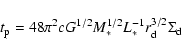
As shown in Icke (2003), the mechanism for the formation of multipolar nebulae only works if the gas is close to isothermal, or in other words, strongly cooling. In order to establish the part of parameter space where the mechanism applies, we need to compare the cooling time scale to three other time scales related to the disk: the precession and growth time scales of the warp, and the shock passing time, where the latter is defined as the time the expanding swept up shell takes to travel to the outer disk radius.
In our simulations we implemented the radiative cooling by interpolation from a tabulated cooling curve taken from Dalgarno & McCray (1972) (see Sect. 5).
In order to calculate an estimate for the cooling time scale, we represent this curve by the following, piecewise linear, approximation:
 |
(3) |
 |
(4) |
| (5) |
 |
(6) |
![\begin{eqnarray*}C_i &= & \frac{1}{\Lambda_i} \left[ \frac{3}{2(1-\alpha_i)} \mu...
...t. (\gamma-1)^{2-\alpha_i} (\gamma+1)^{-(3-2\alpha_i)} \right] ,
\end{eqnarray*}](/articles/aa/full/2005/48/aa1971-04/img74.gif)
 |
(7) |
![\begin{figure}
\par\includegraphics[width=8.8cm,clip]{1971fig2.eps}
\end{figure}](/articles/aa/full/2005/48/aa1971-04/img92.gif) |
Figure 2:
Plot of |
| Open with DEXTER | |
Besides implementing the proper initial and boundary conditions we also added our own cooling module to the code in order to model radiative cooling using a cooling curve (Dalgarno & McCray 1972; Mellema et al. 2002). This curve gives the energy loss rate as a function of temperature for a low density gas in collisional ionization equilibrium. The radiative losses were implemented through operator splitting and if the time step required by the hydrodynamics was larger than the cooling time, the former was subdivided into smaller steps when calculating the cooling.
The temperature ![]() of the environment was kept at its initial equilibrium value by introducing a heating term with a linear dependency on the density, as photo-electric heating would have.
The temperature
of the environment was kept at its initial equilibrium value by introducing a heating term with a linear dependency on the density, as photo-electric heating would have.
The temperature ![]() of the disk was chosen such that it was in pressure equilibrium with the environment.
Furthermore, we made sure no grid cell could obtain a temperature below a minimum value of
of the disk was chosen such that it was in pressure equilibrium with the environment.
Furthermore, we made sure no grid cell could obtain a temperature below a minimum value of ![]() .
.
To construct the warped disk, Eq. (2) was combined with a constant "flare angle''
![]() ,
and a proper value for A.
The outer disk radius
,
and a proper value for A.
The outer disk radius ![]() was taken to be larger than
was taken to be larger than
![]() (cf. Eq. (1)) and the disk was given a constant number density
(cf. Eq. (1)) and the disk was given a constant number density ![]() .
The environment was given a constant number density
.
The environment was given a constant number density ![]() .
The spherical wind was implemented as an interior boundary condition and given a 1/r2 density profile, outer radius
.
The spherical wind was implemented as an interior boundary condition and given a 1/r2 density profile, outer radius ![]() ,
and a constant wind velocity
,
and a constant wind velocity ![]() .
The pressure was calculated from an equation of state with a constant adiabatic index
.
The pressure was calculated from an equation of state with a constant adiabatic index ![]() .
.
Both the module to construct the initial conditions as well as the cooling curve module are available from the authors upon request.
To check the implementation of the wind-disk interaction model into the AMR code described above, we repeated a number of the two-dimensional calculations previously done by Icke (2003). Since in his simulations a different solver (FCT/LCD) for the hydrodynamic equations was used, and the shape of small scale structures in the outcome of the calculations depend on turbulent processes in the gas, the two-dimensional comparison simulations did not agree in every single detail, but the overall point-symmetric morphologies found, were similar in both simulations.
To see the effects of more realistic cooling, we also ran some simulations with the cooling curve module and an adiabatic index
![]() .
At the start of each simulation, the cooling time is already smaller than the hydrodynamical time scale, so the bubble is in the momentum driven stage from the outset.
Since the cooling scales with the density squared and the density in the swept up shell can only increase with time, the cooling gets more efficient as the simulation progresses, and therefore the bubble remains momentum driven throughout the entire simulation.
To fully resolve the developing bow shock and instabilities in these calculations required a fairly high (effective) resolution of 20482 cells.
All two-dimensional simulations used either a small value for the adiabatic index or the cooling curve module, both resulting in momentum driven shells.
See Table 1 for information on the initial parameters.
For all two-dimensional simulations with cooling applied through the cooling curve module we used the following parameters:
.
At the start of each simulation, the cooling time is already smaller than the hydrodynamical time scale, so the bubble is in the momentum driven stage from the outset.
Since the cooling scales with the density squared and the density in the swept up shell can only increase with time, the cooling gets more efficient as the simulation progresses, and therefore the bubble remains momentum driven throughout the entire simulation.
To fully resolve the developing bow shock and instabilities in these calculations required a fairly high (effective) resolution of 20482 cells.
All two-dimensional simulations used either a small value for the adiabatic index or the cooling curve module, both resulting in momentum driven shells.
See Table 1 for information on the initial parameters.
For all two-dimensional simulations with cooling applied through the cooling curve module we used the following parameters:
![]() ,
,
![]() ,
,
![]() ,
,
![]() ,
,
![]() ,
,
![]() AU,
AU,
![]() ,
and
,
and ![]() .
For the calculation of
.
For the calculation of
![]() we used
we used
![]() which is of the same order as the value of 100 AU we used in the simulations.
Note that, for this parameter choice, the Shakura-Sunyaev parameter
which is of the same order as the value of 100 AU we used in the simulations.
Note that, for this parameter choice, the Shakura-Sunyaev parameter
![]() ,
obeys
,
obeys
![]() ,
as is required (see e.g. Pringle 1981).
Also note that, in the simulations, the mass loss rate of the wind
,
as is required (see e.g. Pringle 1981).
Also note that, in the simulations, the mass loss rate of the wind
![]() is a function of
is a function of
![]() ,
such that at
,
such that at
![]() the wind density is set equal to the initial environment density, i.e.
the wind density is set equal to the initial environment density, i.e.
![]() ,
which renders Eq. (11) independent of
,
which renders Eq. (11) independent of
![]() (as is reflected in the constant
(as is reflected in the constant
![]() in Table 1 for different values of
in Table 1 for different values of ![]() ).
The disk mass corresponding to these numbers is quite modest, only
).
The disk mass corresponding to these numbers is quite modest, only
![]()
![]() .
This shows that the mechanism does not require excessive conditions to operate.
.
This shows that the mechanism does not require excessive conditions to operate.
For the runs that were done with the cooling curve module we find that, apart from the formation of the, by now familiar, point-symmetric lobes, the outer shell of swept up gas is much thinner and unstable due to the effective cooling at higher densities. It developes into a number of smaller lobes merging with one another as the shell expands (Fig. 3). Furthermore, the more effective the cooling, the more elongated the lobes created by the bow shock become.
Table 1: Parameters for the two- and three-dimensional runs.
![\begin{figure}
\par\includegraphics[width=8.8cm,clip]{1971fig3.eps}
\end{figure}](/articles/aa/full/2005/48/aa1971-04/img128.gif) |
Figure 3:
Color scale plot of |
| Open with DEXTER | |
Due to the cooling of the gas, the swept up shell is highly compressed and therefore thin, and the ram pressure from the wind directly drives the shell outwards, which are necessary ingredients for the bow shock to produce the lobes. When the cooling is very effective, the shell gets so thin that it becomes unstable, and develops into a number of smaller lobes. Ultimately, when the density of the disk is not too high, the wind breaks through the concave part of the disk, producing another pair of lobes (Fig. 3).
Since the true bow shock is a three-dimensional structure and the disk is warped, the shape of the disk seen in a two-dimensional vertical cut at different azimuthal angles ![]() changes such that the concave side of the disk turns into the convex side and vice versa for increasing
changes such that the concave side of the disk turns into the convex side and vice versa for increasing ![]() .
.
As was pointed out above, the interaction between a spherical wind and a warped disk is point-symmetric by nature, and it is therefore intrinsically three-dimensional. The two-dimensional calculations should therefore be regarded as trial calculations that show the underlying principles of the interaction but, due to the slab symmetry of these two-dimensional simulations which does not correctly capture the point-symmetry of the problem, can not be used to derive any observable morphologies or position-velocity diagrams. So, to truly understand the emerging point-symmetric structure of this interaction, it is necessary to carry out fully three-dimensional simulations.
We ran wind-disk simulations in three dimensions on a Cartesian grid with an effective resolution of 5123 using six levels of refinement![]() .
For our largest calculations we needed approximately 24 h on 64 nodes of an SGI Origin 3800 system, where each node consists of a 500 MHz R14000 CPU with 1 Gbyte of memory.
At the end of each simulation,
.
For our largest calculations we needed approximately 24 h on 64 nodes of an SGI Origin 3800 system, where each node consists of a 500 MHz R14000 CPU with 1 Gbyte of memory.
At the end of each simulation, ![]() 30% of the domain is refined to the highest level, taking all the memory available.
This means that if one would like to follow the simulation for a longer evolutionary time by using a larger domain, and keeping the same (effective) resolution, one should increase the number of nodes accordingly.
30% of the domain is refined to the highest level, taking all the memory available.
This means that if one would like to follow the simulation for a longer evolutionary time by using a larger domain, and keeping the same (effective) resolution, one should increase the number of nodes accordingly.
Since we found in our two-dimensional calculations that simulations with cooling applied through a cooling curve did not result in a qualitatively different morphological outcome compared to calculations with a low value for the adiabatic index, we opted not to use the cooling curve module during our three-dimensional simulations to save on computing time.
Like in the two-dimensional simulations, we used a disk radius of
![]() ,
a wind velocity of
,
a wind velocity of
![]() and a computational domain of
and a computational domain of
![]() .
See Table 1 for a summary of the simulation parameters and resulting timescales.
.
See Table 1 for a summary of the simulation parameters and resulting timescales.
![\begin{figure}
\par\includegraphics[width=6.2cm,clip]{1971fig4.eps}
\end{figure}](/articles/aa/full/2005/48/aa1971-04/img134.gif) |
Figure 4:
Isosurfaces for a density value of
|
| Open with DEXTER | |
In Fig. 5 we show cuts through the centre of the data cube at different times during the simulation. One sees that the point-symmetric structure again emerges, and that the bow shock produces multiple lobes, as in the two-dimensional simulations. To visualize the three-dimensional shape of the swept up shell, corresponding isosurfaces are also shown (Fig. 4).
Since it is the bow shock that drives the shaping of the bubble, any extra small scale instabilities resulting from the extra degree of freedom of our three-dimensional simulations are of relatively little importance. However, one difference between the two-dimensional and the three-dimensional calculations is the way in which the small scale lobes can merge along the surface of the swept up shell, but this does not alter the global shape of the bubble. Also, the extra degree of freedom prevents the wind from breaking through the concave part of the disk, in contrast to what was found from the two-dimensional simulations.
We derived synthesized H![]() images by projecting the three-dimensional data cube onto the plane of the sky.
We integrated the density squared along the line of sight and used this as an estimate for the emission.
In Fig. 6 we present an overview of the point-symmetric shapes we found.
Varying the projection angle produces a plethora of morphologies ranging from clearly quadrupolar (e.g. Fig. 6
images by projecting the three-dimensional data cube onto the plane of the sky.
We integrated the density squared along the line of sight and used this as an estimate for the emission.
In Fig. 6 we present an overview of the point-symmetric shapes we found.
Varying the projection angle produces a plethora of morphologies ranging from clearly quadrupolar (e.g. Fig. 6
![]() )
to multipolar (e.g. Fig. 6 (120,020)).
We can also chose our projection angle such that a more bipolar-like shape emerges, see e.g. Fig. 6 (160,080), or even an almost round shape (Fig. 6 (140,120)).
)
to multipolar (e.g. Fig. 6 (120,020)).
We can also chose our projection angle such that a more bipolar-like shape emerges, see e.g. Fig. 6 (160,080), or even an almost round shape (Fig. 6 (140,120)).
In Fig. 7 the kinematical data in the form of position-velocity diagrams is presented.
These diagrams correspond to the H![]() images of Fig. 6, where, for each diagram, the "slit'' was positioned at the centre of the image and ran in the vertical direction.
To be representative for current observations, we convolved the position-velocity diagrams with two-dimensional Gaussians with a FWHM of
images of Fig. 6, where, for each diagram, the "slit'' was positioned at the centre of the image and ran in the vertical direction.
To be representative for current observations, we convolved the position-velocity diagrams with two-dimensional Gaussians with a FWHM of
![]() along the velocity axis, and a FWHM of
along the velocity axis, and a FWHM of
![]() along the position axis (assuming a distance of
along the position axis (assuming a distance of
![]() to the nebula).
One sees that the point-symmetry is also retained in these diagrams.
We present larger versions of three of our
to the nebula).
One sees that the point-symmetry is also retained in these diagrams.
We present larger versions of three of our
![]() images and their corresponding position-velocity diagrams in Fig. 8.
images and their corresponding position-velocity diagrams in Fig. 8.
![\begin{figure}
\par\includegraphics[height=21cm,clip]{1971fig5.eps}
\end{figure}](/articles/aa/full/2005/48/aa1971-04/img141.gif) |
Figure 5:
Color scale plots of |
| Open with DEXTER | |
![\begin{figure}
\par\includegraphics[width=17cm,clip]{1971fig6.eps}
\end{figure}](/articles/aa/full/2005/48/aa1971-04/img143.gif) |
Figure 6:
Grey scale plots of the synthesized H |
| Open with DEXTER | |
![\begin{figure}
\par\includegraphics[width=17cm,clip]{1971fig7.eps}
\end{figure}](/articles/aa/full/2005/48/aa1971-04/img147.gif) |
Figure 7:
Grey scale plots of the synthesized position-velocity diagrams corresponding to the
|
| Open with DEXTER | |
Whether the shell remains momentum driven in the long term when it expands into a 1/r2 environment depends on parameters like the velocity and mass loss rate of the evolving fast wind, and the actual density distribution in the surrounding medium left behind by the earlier AGB phase.
For example, detailed radiation hydrodynamical calculations performed by Mellema (1994), taking an evolving fast wind and ionization effects into account, showed that there is a transition from momentum to energy driven flow at ![]() 1000 yr.
We therefore expect the multipolar shape of the bubble aquired in the early stages through our mechanism to persist for at least this long a period.
Thus we may also, although tentatively, since the fast wind velocity is expected to increase in time which may alter the morphology of the bubble, compare our results to more evolved PNe.
So, if one assumes that the bubble will expand self-similarly, it will have a size of
1000 yr.
We therefore expect the multipolar shape of the bubble aquired in the early stages through our mechanism to persist for at least this long a period.
Thus we may also, although tentatively, since the fast wind velocity is expected to increase in time which may alter the morphology of the bubble, compare our results to more evolved PNe.
So, if one assumes that the bubble will expand self-similarly, it will have a size of ![]() 10 000 AU (for a PN of
10 000 AU (for a PN of ![]() 10'' at a distance of 1 kpc) at
10'' at a distance of 1 kpc) at
![]() yr, which are reasonable values for observed PNe.
yr, which are reasonable values for observed PNe.
When comparing our H![]() images to observed objects, good candidates that can be accommodated by our model are the quadrupolar PNe K3-24 (Manchado et al. 1996) and NGC 7026 (Solf & Weinberger 1984; Cuesta et al. 1996), and the proto-PNe M1-26 and M4-18 (de Marco & Crowther 1999; Sahai & Trauger 1998).
Although nebulae as compact as those in our models have not yet been observed in sufficient detail, the morphological similarity with the more evolved objects just mentioned suggests that they represent early stages of these.
images to observed objects, good candidates that can be accommodated by our model are the quadrupolar PNe K3-24 (Manchado et al. 1996) and NGC 7026 (Solf & Weinberger 1984; Cuesta et al. 1996), and the proto-PNe M1-26 and M4-18 (de Marco & Crowther 1999; Sahai & Trauger 1998).
Although nebulae as compact as those in our models have not yet been observed in sufficient detail, the morphological similarity with the more evolved objects just mentioned suggests that they represent early stages of these.
Observed position-velocity diagrams for NGC 7026 are presented in Cuesta et al. (1996), together with a rather ad-hoc kinematical model. Upon comparison of our position-velocity diagrams with the observed ones we find qualitatively similar structures, strengthening the validity of our model. For K3-24 and the two proto-PNe mentioned, kinematical data are unfortunately not (yet) available. Another interesting property of observed point-symmetric PNe is that not only the imagery, but also the position-velocity diagrams, show evidence of point-symmetry (e.g. Harman et al. 2004; Guerrero et al. 1999), like we find in our synthetic position-velocity diagrams.
From a calculation of the different timescales of the problem, we determined the boundaries of our parameters space. We found that, although stellar evolution models limit the freedom of choice for a number of parameters, the scaling of the time scales is such that one can always find a proper set of physical parameters.
The influence of more realistic radiative cooling using a cooling curve was investigated, and it was found that, in order to resolve the bow shock that generates the protruding point-symmetric lobes, high resolution simulations were required. Furthermore, the resulting morphologies of the wind blown bubbles found in these two-dimensional simulations using a cooling curve did not differ qualitatively from the ones found in the simulations where simplified cooling was applied through the use of a low value of the adiabatic index. Therefore, we used the latter, computationally less expensive cooling strategy, for our three-dimensional runs.
When analyzing the results from the three-dimensional calculations, we found that our model produces a wide variety of morphologies, ranging from multipolar to quadrupolar and bipolar.
All these shapes were extracted from one single time frame of one single calculation by systematically choosing a number of different projection angles for the data cube.
Besides these synthetic H![]() images, we made the corresponding position-velocity diagrams, which also clearly show the point-symmetry of the model.
images, we made the corresponding position-velocity diagrams, which also clearly show the point-symmetry of the model.
By comparing a number of observed (proto-)PNe with these morphological and kinematical results, four compelling cases were found. These are the quadrupolar PNe K3-24 and NGC 7026, and the multipolar proto-PNe M1-26 and M4-18. Since for K3-24, M1-26, and M4-18 kinematical data is not available, we could not compare our position-velocity diagrams with ones for these objects, so, to further test and constrain our model, it would be very interesting if this data could be obtained.
The method to arrive at the synthetic H![]() images presented in this paper does not include the effects that absorption may have.
Absorption effects may change the resulting image for those lines of sight where the swept up shell becomes optically thick.
In order to facilitate such a more detailed comparison, projection models of radiative solutions taking absorption into account are currently being calculated using a newly developed raytrace algorithm especially suited for the AMR data structures of the Flash code (Rijkhorst et al. 2005).
Furthermore, since this paper presents one three-dimensional result only, it will be of interest to run more models with different wind-disk parameters to provide insight into the variation in resulting morphologies.
We will report on these matters in a future publication.
images presented in this paper does not include the effects that absorption may have.
Absorption effects may change the resulting image for those lines of sight where the swept up shell becomes optically thick.
In order to facilitate such a more detailed comparison, projection models of radiative solutions taking absorption into account are currently being calculated using a newly developed raytrace algorithm especially suited for the AMR data structures of the Flash code (Rijkhorst et al. 2005).
Furthermore, since this paper presents one three-dimensional result only, it will be of interest to run more models with different wind-disk parameters to provide insight into the variation in resulting morphologies.
We will report on these matters in a future publication.
![\begin{figure}
\par\includegraphics[width=8.8cm,clip]{1971fig8.eps}
\end{figure}](/articles/aa/full/2005/48/aa1971-04/img149.gif) |
Figure 8:
Larger versions of three synthesized H |
| Open with DEXTER | |
Acknowledgements
V.I. expresses his gratitude to Raghvendra Sahai and Hugo Schwarz for lively discussions that were the primary cause for taking up this subject.We would like to thank the referee, Vikram Dwarkadas, for pointing out a shortcoming in our original calculation of the cooling time scale.
The software used in this work was in part developed by the DOE-supported ASC/Alliance Center for Astrophysical Thermonuclear Flashes at the University of Chicago.
Our work was sponsored by the National Computing Foundation (NCF) for the use of supercomputer facilities, with financial support from the Netherlands Organization for Scientific Research (NWO), under grant number 614.021.016.
QuickTime Player is required
emissionDiagram.avi
emissionDiagram.mov