A&A 444, 233-244 (2005)
DOI: 10.1051/0004-6361:20052748
A. Verdini1 - M. Velli1 - S. Oughton2
1 - Dipartimento di Astronomia
e Scienza dello Spazio,
Firenze,
Italy
2 - Department of Mathematics,
University of Waikato,
Private Bag 3105,
Hamilton,
New Zeland
Received 24 January 2005 / Accepted 21 June 2005
Abstract
We investigate the nonlinear evolution of Alfvén waves in a
radially stratified isothermal atmosphere with wind, from the
atmospheric base out to the Alfvénic point. Nonlinear interactions,
triggered by wave reflection due to the atmospheric gradients, are assumed
to occur mainly in directions perpendicular to the mean radial magnetic
field. The nonlinear coupling between waves propagating in opposite
directions is modeled by a phenomenological term, containing an
integral turbulent length scale, which acts as a
dissipative coefficient for waves of a given frequency.
Although the wind acceleration profile is not determined self-consistently
one may estimate the dissipation rate inside the
layer and follow the evolution of an initial frequency spectrum.
Reflection of low frequency waves drives dissipation across the whole
spectrum, and
steeper gradients, i.e. lower coronal temperatures,
enhance the dissipation rate.
Moreover, when reasonable wave amplitudes are considered,
waves of all frequencies damp at the same rate and the spectrum is not
modified substantially during propagation. Therefore the
sub-Alfvénic coronal layer
acts differently when waves interact nonlinearly, no longer behaving
as a frequency dependent filter once reflection-generated nonlinear
interactions are included,
at least within the classes of models discussed here.
Key words: magnetohydrodynamics (MHD) - turbulence - waves
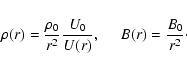
The main difficulties one has to face for the development of such a scenario is the nature of the nonlinear interactions for the incompressible Alfvén mode. Among the many wave-modes generated by photospheric oscillations, Alfvén waves are the most likely to survive into the corona (Hollweg 1978), although other modes may be generated throughout the atmosphere. Analysis of observed oscillations in coronal structures may eventually lead to their identification (De Moortel et al. 2002a,b), but we concentrate here on Alfvén waves, since they are the dominant modes observed in the solar wind. It is well known that nonlinear terms couple Alfvén waves propagating in opposite directions. Note, however, that in the fast solar wind, outwardly propagating modes seem to dominate (Smith et al. 1995).
The inhomogeneities of the ambient medium suggest a solution for this apparent contradiction between dominantly unidirectional propagation and development of nonlinear interactions (Velli et al. 1989). Variations of the group velocity of the wave (the sum of Alfvén and wind speed gradients) linearly couple the outgoing and ingoing waves producing one from the other and furnishing the trigger for nonlinear interactions to take place. Intensive studies of this mechanism have been carried out in terms of the dynamical time scales which enter the governing equation, while the anisotropic nature of the problem was handled naturally in the context of a Reduced Magneto-Hydrodynamics description (RMHD hereafter) which allows a correct treatment of nonlinear terms (Oughton et al. 2001; Dmitruk & Matthaeus 2003; Dmitruk et al. 2002,2001a; Oughton et al. 2004). This kind of approach has led to the understanding of the ordering of the characteristic times which should effectively favor the development of a turbulent cascade in planes perpendicular to the direction of wave propagation (along the magnetic field) and the efficiency of dissipation. Due to the complexity of the equations describing the propagation of large amplitude Alfvén waves in an inhomogeneous moving medium these analyses were developed in a static stratified atmosphere where the profiles of the ambient magnetic field and the density of the medium were imposed in order to produce the Alfvén velocity gradients which, ultimately, determine the amount of reflection inside the simulation box.
Other authors (Moore et al. 1991; Krogulec & Musielak 1998; Velli 1993; Cranmer & van Ballegooijen 2005; Lou & Rosner 1994; Similon & Zargham 1992; Heinemann & Olbert 1980; Velli et al. 1991; Leroy 1980; Mangeney et al. 1991; Grappin et al. 1991; Krogulec et al. 1994; Leroy 1981, but also Dmitruk et al. 2001b for a phenomenological nonlinear model) have focused their attention on the linear theory of wave propagation.
Here, three main features have proved to be essential: first, the geometry of the medium, since the profile of Alfvén speed is strongly affected by the structure of the flux tubes in which waves are supposed to propagate; second, the extent of the atmosphere whose global stratification profile determines the transmission, since it is the entire profile of the Alfvén speed, and not simply its local variation, which determines whether or not a wave at a given frequency is capable of escaping at the top of the atmosphere; third, the presence of a wind which separates the atmosphere into two parts. The Alfvén critical point (the distance from the sun at which the wind speed equals the Alfvén speed) represents a natural separation between an internal region where the wind is slow and affects the propagation of the waves only slightly (at least at high frequencies) and an outer region, beyond the critical point, where waves are advected outwards by the wind regardless of their original propagation direction. Even if in the very low corona one might expect the effect of a bulk flow to be negligible, it was shown (Heinemann & Olbert 1980; Velli 1993; Jokipii & Kota 1989) that the wind speed reduces the reflection inside the atmosphere for low frequency waves, carrying them out through the Alfvénic critical point (beyond which they can not propagate backwards), and hence enhancing their transmission.
The aim of this paper is to investigate nonlinear effects on wave propagation once the background medium and the entire (lower) atmosphere are taken into account. Following Dmitruk et al. (2001b), we choose a constant or radially expanding transverse dissipative length scale and a phenomenological nonlinear coupling term. This allows us to give a preliminary estimate of dissipation caused by the turbulent cascade of counter-propagating Alfvén waves. Introducing such a term still allows wave propagation to be handled in a relatively simple way and, despite the roughness of the model, allows one to gain insight into the relative importance of the three features listed above when dissipative nonlinear effects are also present.
The paper is structured as follows. First we review the equations which describe Alfvén wave propagation in an inhomogeneous moving medium, then we briefly review the results derived from linear propagation and finally we introduce the phenomenological terms, which split the nonlinear analysis into two models, one in which interactions take place only among waves of the same frequency, and the other in which interactions between different frequencies are taken into account. For parameter space, particular attention is paid to the solar case. Finally we review these results and discuss the development of a more realistic model.
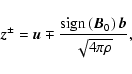
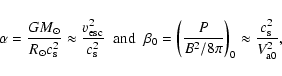
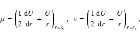
The isothermal atmosphere is completely defined by setting the values
for temperature, density and magnetic field intensity at the base,
together with the mass and radius of the central object (![]() and
and ![]() ).
The wind speed and Alfvén speed profiles (and their
derivatives) depend on the two parameters
).
The wind speed and Alfvén speed profiles (and their
derivatives) depend on the two parameters
![]() ,
the non dimensional scale height, and
,
the non dimensional scale height, and ![]() ,
the
plasma parameter at the base,
,
the
plasma parameter at the base,
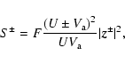
It is natural
to define the top of the atmosphere at the Alfvénic critical point
(labeled with c), since only an outward flux (
![]() )
remains at this point, so that
a transmission (
)
remains at this point, so that
a transmission (![]() )
and a reflection (
)
and a reflection (![]() )
coefficient may be
defined:
)
coefficient may be
defined:
Assuming
![]() ,
expressing length in unit
of
,
expressing length in unit
of ![]() ,
velocities in units of sound speed, and frequencies in unit of
,
velocities in units of sound speed, and frequencies in unit of
![]() ,
the non-dimensional form for
Eq. (1), linearized and reduced for the spherical symmetry
case, finally becomes:
,
the non-dimensional form for
Eq. (1), linearized and reduced for the spherical symmetry
case, finally becomes:
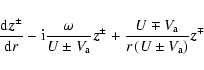
 |
(9) |
![\begin{figure}
\par\includegraphics[height=4.4cm,width=8.4cm,clip]{fig/2748fg1.eps}
\end{figure}](/articles/aa/full/2005/46/aa2748-05/img100.gif) |
Figure 1:
Transmission coefficient as function of frequency in
logarithmic scale for isothermal layers of different
temperatures. The value of |
| Open with DEXTER | |
 |
(11) |
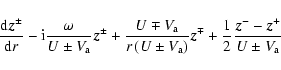
The form of the nonlinear term may be heuristically derived from the following
arguments.
When Eq. (1) is Fourier decomposed (
![]() )
nonlinear terms
couple several wave numbers in the k-space.
When a strong magnetic field (
)
nonlinear terms
couple several wave numbers in the k-space.
When a strong magnetic field (![]() in velocity units) is present,
the propagation time of the Alfvén waves
in velocity units) is present,
the propagation time of the Alfvén waves
![]() is
equal or shorter than the characteristic time-scale for nonlinear
interaction
is
equal or shorter than the characteristic time-scale for nonlinear
interaction
![]() over most
of the Fourier space,
the nature of
the nonlinear cascade is highly anisotropic, developing preferentially
in planes perpendicular
to the direction of the mean field
(Oughton et al. 1994; Shebalin et al. 1983; Goldreich & Sridhar 1995).
It is then useful to decompose local wavenumber in projections
along the magnetic field (
over most
of the Fourier space,
the nature of
the nonlinear cascade is highly anisotropic, developing preferentially
in planes perpendicular
to the direction of the mean field
(Oughton et al. 1994; Shebalin et al. 1983; Goldreich & Sridhar 1995).
It is then useful to decompose local wavenumber in projections
along the magnetic field (
![]() )
and in the perpendicular
planes (
)
and in the perpendicular
planes (
![]() )
because energy transfer occurs only among the latter,
so that Fourier decomposition is exploited only in
)
because energy transfer occurs only among the latter,
so that Fourier decomposition is exploited only in
![]() .
When small fluctuations are considered
(
.
When small fluctuations are considered
(
![]() )
these
arguments lead to the so called RMHD description which can be derived
as an expansion of the usual MHD equations in the small parameter
)
these
arguments lead to the so called RMHD description which can be derived
as an expansion of the usual MHD equations in the small parameter
![]() with the restriction
with the restriction
![]() (see Oughton et al. 2004 and
reference therein for more details on RMHD), in which variations along
the perpendicular directions are decoupled from those along the
magnetic field (
(see Oughton et al. 2004 and
reference therein for more details on RMHD), in which variations along
the perpendicular directions are decoupled from those along the
magnetic field (
![]() ,
with
,
with
![]() ).
We can describe the global effect of this perpendicular
cascade by means
of two quantities at the large scales, namely
an integral scale
).
We can describe the global effect of this perpendicular
cascade by means
of two quantities at the large scales, namely
an integral scale
![]() ,
giving the dimension of the greatest eddies in which
energy is injected, and the average velocity difference (
,
giving the dimension of the greatest eddies in which
energy is injected, and the average velocity difference (![]() )
among points belonging to the same eddy, which in RMHD
turbulence also contains magnetic field fluctuations in
velocity units (
)
among points belonging to the same eddy, which in RMHD
turbulence also contains magnetic field fluctuations in
velocity units (
![]() ). Identifying these two
quantities with the integral turbulent length (
). Identifying these two
quantities with the integral turbulent length (
![]() )
and the
fluctuations' amplitude of the Elsässer fields we can construct a
characteristic timescale
)
and the
fluctuations' amplitude of the Elsässer fields we can construct a
characteristic timescale
![]() which
accounts for nonlinear turbulent interactions in
Eq. (1)
(see Dobrowolny et al. 1980 for a more accurate
derivation).
which
accounts for nonlinear turbulent interactions in
Eq. (1)
(see Dobrowolny et al. 1980 for a more accurate
derivation).
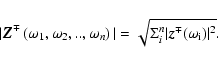
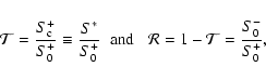
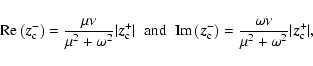
Multiplying the above Eq. (12) by the
complex conjugate
![]() one obtains the evolution equations for
the Elsässer energies at a given frequency
one obtains the evolution equations for
the Elsässer energies at a given frequency
![]() .
On its RHS one finds
.
On its RHS one finds
![]() ,
which
acts as a sink for the energy of a given mode.
To quantify
the relative importance of various couplings we first consider only
nonlinear interactions between counter-propagating waves with the same
frequency.
Thereafter we consider the more realistic case of
different couplings between a fundamental frequency (a very low
frequency, sometimes called the quasi-2D component,
labeled with index 0) and other higher frequencies labeled
as interacting (index i).
,
which
acts as a sink for the energy of a given mode.
To quantify
the relative importance of various couplings we first consider only
nonlinear interactions between counter-propagating waves with the same
frequency.
Thereafter we consider the more realistic case of
different couplings between a fundamental frequency (a very low
frequency, sometimes called the quasi-2D component,
labeled with index 0) and other higher frequencies labeled
as interacting (index i).
In both cases, once nonlinear terms are introduced we loose the scaling feature of the linearized equation for which given an increment of a factor f in the amplitudes at the critical point we have an equal increment f for the values at the base. Hence, to get realistic values of velocity and magnetic field fluctuations at the base of the atmosphere, we have to tune the amplitude of the outgoing wave imposed at the Alfvénic critical point (since the equations are still integrated backward) for every frequency and coupling considered.
In the following we first present the results concerning the self-interacting
case,
where only monochromatic waves interact,
then we shall consider modification to dissipation induced by
different coupling among two or three frequencies.
As model parameters we choose
![]() corresponding to
temperatures for an isothermal layer above the sun's surface
ranging from approximately
corresponding to
temperatures for an isothermal layer above the sun's surface
ranging from approximately
![]() (
(![]() )
to
)
to
![]() (
(![]() ), and we
fix the value of the plasma parameter at
), and we
fix the value of the plasma parameter at
![]() for every
temperature; thus, at the base of the atmosphere the Alfvén speed is
always five times the sound speed.
Finally we set the value of the phenomenological turbulent length
for every
temperature; thus, at the base of the atmosphere the Alfvén speed is
always five times the sound speed.
Finally we set the value of the phenomenological turbulent length
![]() ,
that is about
,
that is about
![]() corresponding to the
average size of the supergranules at coronal level which is maintained
at a constant value through the entire atmosphere.
corresponding to the
average size of the supergranules at coronal level which is maintained
at a constant value through the entire atmosphere.
| |
Figure 2:
Total wave action density normalized to the base value as
a function of radius in |
| Open with DEXTER | |
The reflection rate depends both on temperature and wave frequency and it
is higher for cooler atmospheres and lower frequency waves.
Moreover, most of the reflection takes place
in the lower atmosphere, where the Alfvén speed
gradients are stronger.
For high enough wave amplitudes, nonlinear terms dominate
over linear ones and the profile of
![]() is determined uniquely by the local reflection rate, which, for cold
atmospheres, is itself dominated by the Alfvén speed gradients.
is determined uniquely by the local reflection rate, which, for cold
atmospheres, is itself dominated by the Alfvén speed gradients.
Ultimately
one expects ![]()
![]() to increase with
to increase with ![]() ,
and
,
and ![]() to decrease faster with radius in the very low atmosphere.
For a given
to decrease faster with radius in the very low atmosphere.
For a given ![]() this behavior should be more pronounced
for low-frequency waves (those suffering stronger reflection) and
consequently high-frequency dissipation should be less sensitive to
temperature variations.
this behavior should be more pronounced
for low-frequency waves (those suffering stronger reflection) and
consequently high-frequency dissipation should be less sensitive to
temperature variations.
![\begin{figure}
\par\includegraphics[height=4.4cm,width=8.6cm,clip]{fig/2748fg4.eps}
\end{figure}](/articles/aa/full/2005/46/aa2748-05/img156.gif) |
Figure 3:
Dissipation efficiency ( |
| Open with DEXTER | |
To investigate the amplitude dependence of the solutions
we consider the case of
a frequency small enough (
![]() )
to remain to the left of
)
to remain to the left of ![]() for all temperatures investigated.
In Fig. 4 the values of the outgoing and ingoing wave
amplitudes at the base are plotted as
a function of the outgoing wave amplitude imposed at the critical
point, i.e.
the energy.
for all temperatures investigated.
In Fig. 4 the values of the outgoing and ingoing wave
amplitudes at the base are plotted as
a function of the outgoing wave amplitude imposed at the critical
point, i.e.
the energy.
![\begin{figure}
\par\includegraphics[height=4.4cm,width=8.8cm,clip]{fig/2748fg5.eps}
\end{figure}](/articles/aa/full/2005/46/aa2748-05/img164.gif) |
Figure 4:
Outgoing and ingoing wave amplitude (solid line)
calculated at the base of the |
| Open with DEXTER | |
![\begin{figure}
\par\includegraphics[height=4.4cm,width=8.6cm,clip]{fig/2748fg6.eps}
\end{figure}](/articles/aa/full/2005/46/aa2748-05/img169.gif) |
Figure 5:
Dissipation efficiency as function of initial outgoing wave
amplitude for
|
| Open with DEXTER | |
![\begin{figure}
\par\includegraphics[height=4.4cm,width=8.2cm,clip]{fig/2748fg7.e...
...m}
\includegraphics[height=4.4cm,width=8.2cm,clip]{fig/2748fg8.eps}
\end{figure}](/articles/aa/full/2005/46/aa2748-05/img173.gif) |
Figure 6:
Flat spectrum.
Left panel. Total wave action density, normalized to the base
value, for the interacting frequencies in
different coupling (labelled with letters, see text),
as function of distance from the atmosphere's base expressed
in unit of |
| Open with DEXTER | |
![\begin{figure}
\par\includegraphics[height=4.5cm,width=8cm,clip]{fig/2748fg9.eps...
...mm}
\includegraphics[height=4.5cm,width=8cm,clip]{fig/2748fg10.eps}
\end{figure}](/articles/aa/full/2005/46/aa2748-05/img174.gif) |
Figure 7: Same as Fig. 6 but for a power-law spectrum at the critical point. |
| Open with DEXTER | |
Since in a decaying power law spectrum most of the energy is retained in
the low frequencies we expect nonlinear interaction to be more
important when such frequencies are involved,
hence we choose
![]() (representative of low
frequencies, say
(representative of low
frequencies, say
![]() )
and
)
and
![]() varying from about
varying from about
![]() to
to
![]() increasing by a factor 10 at each step. Specifically, we consider the
four couplings,
increasing by a factor 10 at each step. Specifically, we consider the
four couplings,
Consider first the flat spectrum case shown in Fig. 6 (left panel).
The general dissipation profile as a function of r is similar to that formed
in Fig. 2 (right panel). The main result here is that higher
frequency waves (b, c ,d) may also dissipate efficiently thanks to their
coupling with the reflected mode of the very low frequency component, so that
all profiles show a significant decrease with distance.
This also has an effect on the decay of the lowest (zero) frequency mode, whose
reflected mode is ultimately the trigger for nonlinear evolution.
When the amplitudes of the higher frequency modes are large (i.e. of the same
order of magnitude of the low frequency mode), they influence the
evolution of the zero frequency reflected component,
which then also affects the zero-frequency outward component,
driving the profiles to convergence as illustrated
in Fig. 6 (right panel): at low amplitudes
![]() differs from
differs from
![]() but at high amplitudes
but at high amplitudes
![]() ,
which means a strong coupling.
,
which means a strong coupling.
Consider now the power-law spectrum illustrated in Fig. 7.
The dissipation profile is the same for all the couplings considered (left
panel).
Now the energy
in the high-frequency waves (mainly propagating outwards) is so small that it
has a negligible effect on the evolution of the zero-frequency mode (no back
reaction) which, in turn, drives the dissipation of all the coupled modes.
On the other hand, in the right panel, one can see that the profiles of
![]() and
and
![]() are
similar to the flat spectrum case and they
begin to converge at almost the same values of
are
similar to the flat spectrum case and they
begin to converge at almost the same values of
![]() .
.
The two parameters, ![]() and
and
![]() ,
determine how strong the
coupling is, independently of the shape of the spectrum.
For a given amplitude at the critical point of the zero-frequency wave,
temperature controls the amount of reflection produced inside the layer,
and hence both the linear coupling
among the counter-propagating waves of a given frequency (i.e. differences in
the waves' evolution due to frequency differences) and the amplitude of the
zero-frequency reflected component (the driver).
One finds that increasing the temperature (decreasing
,
determine how strong the
coupling is, independently of the shape of the spectrum.
For a given amplitude at the critical point of the zero-frequency wave,
temperature controls the amount of reflection produced inside the layer,
and hence both the linear coupling
among the counter-propagating waves of a given frequency (i.e. differences in
the waves' evolution due to frequency differences) and the amplitude of the
zero-frequency reflected component (the driver).
One finds that increasing the temperature (decreasing ![]() )
the coupling becomes
weaker for a low
)
the coupling becomes
weaker for a low
![]() and
stronger for a high
and
stronger for a high
![]() ,
depending on which of the
two above features is dominant.
For a given coupling,
,
depending on which of the
two above features is dominant.
For a given coupling,
![]() ,
at a given temperature,
the zero frequency wave amplitude imposed at the critical point
determines the importance of
nonlinear terms (see Fig. 4), and hence the nonlinear coupling
among the waves (the evolution independent of frequencies).
Increasing
,
at a given temperature,
the zero frequency wave amplitude imposed at the critical point
determines the importance of
nonlinear terms (see Fig. 4), and hence the nonlinear coupling
among the waves (the evolution independent of frequencies).
Increasing
![]() increases the strength of the
coupling.
increases the strength of the
coupling.
Two factors determine the rate of dissipation for the
coupled waves.
The first, as in the self-interacting case, comes from inward propagating wave
generation and dissipation. Since this mechanism is driven by reflection it is
a characteristic feature of low-frequency waves (the fundamental) and it acts
approximately as in the previous analysis, hence it depends
most on the low-frequency initial wave amplitude.
The second comes from the form chosen for the coupling where
high-frequency waves can be dissipated too.
They are essentially propagating
outward and their main effect is to dissipate the reflected
low-frequency wave.
The ratio formed with two coupled wave amplitudes
controls the relevance of this second aspect.
For
![]() ,
reflected
waves are suppressed as soon as they are generated and the dissipation rates
of
,
reflected
waves are suppressed as soon as they are generated and the dissipation rates
of
![]() is increased compared to the self-interacting case
but that one of
is increased compared to the self-interacting case
but that one of
![]() is reduced.
When
is reduced.
When
![]() the outward
high-frequency wave has little capability in suppressing the reflected waves
and both dissipation rates are almost completely determined by the
fundamental mode:
no matter what the coupling is, dissipation efficiency is practically the
same for the coupled waves (strength of the coupling) and also for all the
couplings formed with different interacting frequencies (negligible effect
of the high frequency waves).
the outward
high-frequency wave has little capability in suppressing the reflected waves
and both dissipation rates are almost completely determined by the
fundamental mode:
no matter what the coupling is, dissipation efficiency is practically the
same for the coupled waves (strength of the coupling) and also for all the
couplings formed with different interacting frequencies (negligible effect
of the high frequency waves).
![\begin{figure}
\par\includegraphics[height=4.2cm,width=8.8cm,clip]{fig/2748fg11....
...}
\includegraphics[height=4.2cm,width=8.8cm,clip]{fig/2748fg12.eps}
\end{figure}](/articles/aa/full/2005/46/aa2748-05/img203.gif) |
Figure 8:
Dissipation efficiency as function of initial outgoing wave
amplitude
|
| Open with DEXTER | |
![\begin{figure}
\par\includegraphics[height=4.3cm,width=8.7cm,clip]{fig/2748fg13....
...}
\includegraphics[height=4.3cm,width=8.7cm,clip]{fig/2748fg14.eps}
\end{figure}](/articles/aa/full/2005/46/aa2748-05/img206.gif) |
Figure 9:
Spectra at the top (dotted line) and the bottom (solid
line) of the atmosphere for three representative initial values of
|
| Open with DEXTER | |
Supported by these arguments we shall study the behavior of efficiency and spectra with respect to "initial'' wave amplitude variation of two representative couplings:
For the intermediate frequency coupling (righthand panel),
the three
curves for the coupled waves follow different profiles and
give evidence of how much coupling strength is frequency dependent:
for the "middle'' frequency (dotted line)
dissipation efficiency soon reaches the fundamental mode regime even
in the coolest atmospheres, while the highest frequency mode
(dashed line) follows almost the same profile as in coupling a.
A major difference between cool and hot atmospheres is the
behavior of the middle frequency which, for low enough initial
amplitude shows a more efficient dissipation than the fundamental
mode. This can be attributed to the wind effect which manifests for
cooler atmospheres and weak nonlinear self-interaction
or coupling (low amplitudes). It separates very low frequency
behavior (wave mainly transmitted, poor dissipation) and intermediate
frequency behavior (wave mainly reflected and strong dissipation).
![\begin{figure}
\par\includegraphics[height=4.3cm,width=8.7cm,clip]{fig/2748fg15....
...}
\includegraphics[height=4.3cm,width=8.7cm,clip]{fig/2748fg16.eps}
\end{figure}](/articles/aa/full/2005/46/aa2748-05/img211.gif) |
Figure 10:
Ratio |
| Open with DEXTER | |
It is then interesting to track the modifications of the imposed (at ![]() )
spectra
back to the base of the atmosphere, for varying "initial'' wave amplitudes.
Only coupling b will be considered, for which one expects greater
modifications.
Figure 9 plots
the spectra
)
spectra
back to the base of the atmosphere, for varying "initial'' wave amplitudes.
Only coupling b will be considered, for which one expects greater
modifications.
Figure 9 plots
the spectra
![]() imposed at the
top of the atmosphere (dotted lines) and the spectra obtained by
integration to the base of the atmosphere (solid lines). Results are shown
for two different temperatures (
imposed at the
top of the atmosphere (dotted lines) and the spectra obtained by
integration to the base of the atmosphere (solid lines). Results are shown
for two different temperatures (
![]() ).
Three representative top-boundary wave amplitudes of the fundamental frequency
are considered whose values are
).
Three representative top-boundary wave amplitudes of the fundamental frequency
are considered whose values are
![]() .
Since we impose a power-law spectrum at the top of the layer
all dotted lines have slope -5/3 and can be
used as reference to see the modification induced by wave
propagation.
It is striking how much the spectra remain unchanged for practically
all the temperature and all the initial amplitude considered and even if
couplings with highest frequency waves are formed (not shown here).
With a more accurate inspection one actually finds that the spectra
change slightly (see for example solid the line marked with diamonds in the
right panel).
The ratio
.
Since we impose a power-law spectrum at the top of the layer
all dotted lines have slope -5/3 and can be
used as reference to see the modification induced by wave
propagation.
It is striking how much the spectra remain unchanged for practically
all the temperature and all the initial amplitude considered and even if
couplings with highest frequency waves are formed (not shown here).
With a more accurate inspection one actually finds that the spectra
change slightly (see for example solid the line marked with diamonds in the
right panel).
The ratio
In Fig. 10 we plot such ratios normalized to the value of
the fundamental mode, i.e.
![]() and
and
![]() (the fundamental being normalized to
its value)
for the cases shown in Fig. 9.
Since the spectrum at the top is fixed by the initial condition,
a normalized
(the fundamental being normalized to
its value)
for the cases shown in Fig. 9.
Since the spectrum at the top is fixed by the initial condition,
a normalized ![]() lower
(greater) than one means the spectrum is steepening (flattering).
lower
(greater) than one means the spectrum is steepening (flattering).
For low initial amplitudes in hot atmospheres the
spectrum becomes flatter at high frequencies, since the coupling is
not so strong and frequency dependence displays its
influence.
As we increase the strength of the coupling, by increasing
![]() ,
differences are smoothed and the spectrum first
adjusts itself to the slope imposed at the top of the atmosphere and
then finally steepens.
The same behavior is observed for the higher
frequency coupling case a (not shown),
so one can attribute such
a general feature to the high temperature atmospheres.
,
differences are smoothed and the spectrum first
adjusts itself to the slope imposed at the top of the atmosphere and
then finally steepens.
The same behavior is observed for the higher
frequency coupling case a (not shown),
so one can attribute such
a general feature to the high temperature atmospheres.
For low temperatures, the picture is more complicated. Frequency
differences are more important and the strength of the coupling is reduced,
the intermediate frequency waves contribute to dissipation with their
self-interacting part so that the spectrum steepens at intermediate
frequencies and flattens at high frequency.
To quantify this tendency, we have calculated the exponent of the resulting
power-law scaling at the base for the low and high frequency branches.
In the worst of the cases (
![]() for
for ![]() in
Fig. 10) the slopes are 1.61 (spectrum steepening) and 1.76
(spectrum flattening) to compare with 1.667, but generally the slope is 1.65
(steepening) or 1.67 (flattering).
One can then conclude that even if the spectra
evolves during propagation the differences between the slopes at the
top and bottom are always very small or even negligible.
in
Fig. 10) the slopes are 1.61 (spectrum steepening) and 1.76
(spectrum flattening) to compare with 1.667, but generally the slope is 1.65
(steepening) or 1.67 (flattering).
One can then conclude that even if the spectra
evolves during propagation the differences between the slopes at the
top and bottom are always very small or even negligible.
Note how for lower ![]() and low amplitude the spectrum is unchanged
by propagation, even though consistent differences in the dissipation
efficiencies of the coupled modes are found.
The origin of such discrepancies is to be found in the
definition of
and low amplitude the spectrum is unchanged
by propagation, even though consistent differences in the dissipation
efficiencies of the coupled modes are found.
The origin of such discrepancies is to be found in the
definition of ![]() which involves total wave action density at
the boundaries of the layer, including a contribution from
inward and outward fluxes at the boundaries which are not simply wave
amplitudes (which indeed determine the spectrum).
One can in fact rewrite
which involves total wave action density at
the boundaries of the layer, including a contribution from
inward and outward fluxes at the boundaries which are not simply wave
amplitudes (which indeed determine the spectrum).
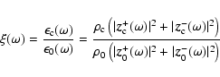
One can in fact rewrite ![]() as follows:
as follows:
![\begin{displaymath}\gamma\approx 1-g(\alpha)\frac{\vert\vec{z}_{\rm c}^+\vert^2}...
...rt^2}{\vert\vec{z}_0^+\vert^2}\left(1-g(\alpha)\right)\right],
\end{displaymath}](/articles/aa/full/2005/46/aa2748-05/img229.gif)
![\begin{displaymath}\xi\approx \frac{\rho_c}{\rho_0}\frac{\vert\vec{z}_{\rm c}^+\...
...frac{\vert\vec{z}_0^-\vert^2}{\vert\vec{z}_0^+\vert^2}\right],
\end{displaymath}](/articles/aa/full/2005/46/aa2748-05/img230.gif) |
(15) |
![\begin{figure}
\par\includegraphics[width=8.8cm,clip]{fig/2748fg17.eps}
\end{figure}](/articles/aa/full/2005/46/aa2748-05/img234.gif) |
Figure 11:
Same as in Fig. 8 for coupling b and
power-law initial spectrum except that
integrations are performed using a spherically expanding turbulent
length
|
| Open with DEXTER | |
For low
![]() ,
dissipation efficiency is considerably
altered (reduced) with respect to the non-expanding case (compare
Figs. 11 and 8).
Since nonlinear term influences are now reduced, we need greater
initial amplitudes to efficiently couple the frequencies considered;
as a consequence the profiles of
,
dissipation efficiency is considerably
altered (reduced) with respect to the non-expanding case (compare
Figs. 11 and 8).
Since nonlinear term influences are now reduced, we need greater
initial amplitudes to efficiently couple the frequencies considered;
as a consequence the profiles of ![]() are shifted to the right with
respect to the non-expanding model (by a factor of 3 or 4).
For coupling a, the plots of
are shifted to the right with
respect to the non-expanding model (by a factor of 3 or 4).
For coupling a, the plots of ![]() show the same kind of
variations as discussed above and the profile of the interacting
frequencies (
show the same kind of
variations as discussed above and the profile of the interacting
frequencies (
![]() and
and
![]() )
again coincides for every
amplitude and temperature. Their values are identical to the high
frequency one in coupling b (dashed lines in Fig. 11).
)
again coincides for every
amplitude and temperature. Their values are identical to the high
frequency one in coupling b (dashed lines in Fig. 11).
If we again construct the ratio ![]() ,
then when we consider high
temperatures we
obtain the same features as in the non-expanding case,
but in the "worst cases''
(low temperature and low amplitudes) differences in the slopes are more
evident suggesting some spectral in such conditions.
,
then when we consider high
temperatures we
obtain the same features as in the non-expanding case,
but in the "worst cases''
(low temperature and low amplitudes) differences in the slopes are more
evident suggesting some spectral in such conditions.
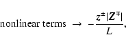
As might be expected, lower temperature atmospheres, with higher gradients, and lower frequency waves allow a stronger dissipation of outwardly propagating waves. On the other hand our results seem to imply that a well developed turbulent spectrum does not change appreciably during propagation.
The dissipation rate has been studied, varying the temperature of the layer and the frequency and amplitude (imposed at the critical point) of the waves. We find that for a given amplitude and frequency, the dissipation rate is stronger in the lower part of the atmosphere and depends strongly on the temperature, which ultimately determines the amount of reflection via the density gradients. As the wave amplitude is increased, the dissipation rate is enhanced, reaching a saturation value which depends on temperature and frequency. Saturation is an effect of nonlinear-dissipative interactions which limit the inward propagating (reflected) wave amplitude once the outgoing amplitude is increased beyond a given value (which also depends on temperature and frequency). Below a critical frequency (whose temperature dependence is negligible), dissipation assumes a constant rate all the way down to "zero-frequency'' fluctuations, while above the critical frequency the dissipation rate tends to zero as frequency is increased, since the amount of reflection decreases with frequency (WKB behavior). The local interaction analysis shows that even if the amplitudes of the inward propagating waves at the base are negligible, continuous reflection due to wind and Alfvén speed gradients can produce significant dissipation (see comments in Fig. 5 at the end of Sect. 3.1); however, only low frequency waves are efficiently dissipated for reasonable wave amplitudes.
We have also investigated
a more realistic calculation, considering non-local interactions,
where an outwardly propagating Alfvén wave is allowed to
interact nonlinearly with the total rms value of inward fluctuations summed
over all frequencies (and vice versa).
Our approach differs from what has been done in a recent paper of
Cranmer & van Ballegooijen (2005) in two related aspects concerning
the nonlinear-dissipative interactions.
We consider the full expression of the wave action density, hence including the
downward propagating flux, or in other words, the nonlinear equations of the
Elsässer fields are integrated simultaneously to include the effect of the
dissipation in a consistent way.
Nonlinear interactions act on both types of
(counterpropagating) waves,
thereby producing the
attenuation of the reflected component which affects the driving of the
global dissipation.
In our analysis, the
description of the total rms value of the fluctuation
is approximated by two or three
representative waves with different frequencies spread across a spectrum, the
"zero frequency'' wave for the low frequencies, and the higher frequencies
selected from spectra with different slopes.
The strength of the coupling, i.e., the total energy in the outward modes at the
lower frequencies (for which reflection is efficient) is crucial for the way in
which energy is dissipated along the spectrum.
If the amplitude of the low frequency wave is high enough (say
![]() at the base for a
at the base for a
![]() atmosphere)
dissipation of all the outward modes is driven by the low-frequency
(quasi-2D) reflected waves: the coupling may be considered strong.
A second important aspect is the
slope of the spectrum or equivalently the relevant energy residing in the higher
frequency waves.
Its effect is to
enable dissipation of the low-frequency reflected component, since there is
little reflected energy at high frequencies, and ultimately to reduce the
dissipation efficiency of all the waves coupled.
In summary, for a given total outward energy, dissipation is more efficient if
the spectra have
higher energies at lower frequencies, i.e. steeper spectral slopes.
atmosphere)
dissipation of all the outward modes is driven by the low-frequency
(quasi-2D) reflected waves: the coupling may be considered strong.
A second important aspect is the
slope of the spectrum or equivalently the relevant energy residing in the higher
frequency waves.
Its effect is to
enable dissipation of the low-frequency reflected component, since there is
little reflected energy at high frequencies, and ultimately to reduce the
dissipation efficiency of all the waves coupled.
In summary, for a given total outward energy, dissipation is more efficient if
the spectra have
higher energies at lower frequencies, i.e. steeper spectral slopes.
Setting the lowest frequency to higher values, say
![]() ,
produces some differences in the results, but the global analysis remains
unchanged.
From Fig. 3 one can guess how the strength of the coupling is
affected and hence how the spectra change. In fact the higher the frequency is,
the lower the amount of reflected waves; hence the lowest frequency wave is
less efficient in driving the dissipation of all the waves coupled.
Imposing the same amplitude at the critical point the strength of the coupling
is lower, linear effects (i.e. differences in the wave
propagation due to different reflection rates) become more important and the
spectra show a somewhat higher modification.
However, increasing the amplitude
of the lowest frequency wave restores the importance of nonlinear terms
(the coupling) which overcome the linear effects.
These considerations remain valid
if one chooses the lowest frequency in the low-frequency plateaus of
the curves in
Fig. 3.
Note that the rightward extension of the plateau increases with increasing wave
amplitude.
,
produces some differences in the results, but the global analysis remains
unchanged.
From Fig. 3 one can guess how the strength of the coupling is
affected and hence how the spectra change. In fact the higher the frequency is,
the lower the amount of reflected waves; hence the lowest frequency wave is
less efficient in driving the dissipation of all the waves coupled.
Imposing the same amplitude at the critical point the strength of the coupling
is lower, linear effects (i.e. differences in the wave
propagation due to different reflection rates) become more important and the
spectra show a somewhat higher modification.
However, increasing the amplitude
of the lowest frequency wave restores the importance of nonlinear terms
(the coupling) which overcome the linear effects.
These considerations remain valid
if one chooses the lowest frequency in the low-frequency plateaus of
the curves in
Fig. 3.
Note that the rightward extension of the plateau increases with increasing wave
amplitude.
We have also considered
a spherically expanding length scale
![]() .
In this case,
the qualitative features discussed above remain essentially the same
(for high enough initial amplitudes).
The main effect of the expansion is to reduce the phenomenological
gradient 1/L(r) entering the nonlinear term of
Eq. (12) as we move further out in the atmosphere so
that dissipation in the higher part of the layer is greatly reduced.
As a result the amount of energy dissipated is decreased and one can
actually attribute differences in the dissipation rate of waves at
different frequencies almost entirely to differences in their
propagation through the low atmosphere where gradients are greater and
hence where most of reflection takes place.
.
In this case,
the qualitative features discussed above remain essentially the same
(for high enough initial amplitudes).
The main effect of the expansion is to reduce the phenomenological
gradient 1/L(r) entering the nonlinear term of
Eq. (12) as we move further out in the atmosphere so
that dissipation in the higher part of the layer is greatly reduced.
As a result the amount of energy dissipated is decreased and one can
actually attribute differences in the dissipation rate of waves at
different frequencies almost entirely to differences in their
propagation through the low atmosphere where gradients are greater and
hence where most of reflection takes place.
Of course, to better understand the spectral evolution in a stratified atmosphere one should also include the chromosphere, the photosphere and the transition region. Here different physical conditions are encountered and it is not clear how the evolution of the waves in these regions affects the development of "Alfvénic turbulence''.
Modeling the deeper stratified layers as
a set of isothermal layer with different temperatures (with a discontinuity
across the transition region)
produces changes of
the parameter ![]() which has been held fixed in our analysis.
In our case, how changes in
which has been held fixed in our analysis.
In our case, how changes in ![]() affect the result may be discussed
qualitatively.
First note that for a given temperature, the wind solutions are selected
(see Eq. (2)) and hence the wind
profile and its gradients remain the same.
As
affect the result may be discussed
qualitatively.
First note that for a given temperature, the wind solutions are selected
(see Eq. (2)) and hence the wind
profile and its gradients remain the same.
As ![]() is increased the Alfvén
speed decreases (still maintaining its characteristic profile,
i.e. a maximum at
is increased the Alfvén
speed decreases (still maintaining its characteristic profile,
i.e. a maximum at ![]() ), its gradients decrease too and the
Alfvén critical point moves to lower radii.
In the linear case the net effect is an enhanced transmission at low
and intermediate frequencies.
When nonlinear interactions are taken into account the
amplitudes must be scaled to get the
same quantitative results, i.e. the same amplitude may be regarded as low in
a high
), its gradients decrease too and the
Alfvén critical point moves to lower radii.
In the linear case the net effect is an enhanced transmission at low
and intermediate frequencies.
When nonlinear interactions are taken into account the
amplitudes must be scaled to get the
same quantitative results, i.e. the same amplitude may be regarded as low in
a high ![]() plasma or high in a low
plasma or high in a low ![]() plasma as far as
the strength of the coupling is concerned because, for a given temperature,
the strength depends entirely on the amount of reflection.
When multiple isothermal layers with different
temperatures and different thicknesses are considered,
other
characteristic length scales and gradients are introduced in the equation
describing the wave propagation.
The transmission properties
of the entire atmosphere are altered, as are the
properties of wave dissipation and the spectral slope
(we leave this question to a following paper).
plasma as far as
the strength of the coupling is concerned because, for a given temperature,
the strength depends entirely on the amount of reflection.
When multiple isothermal layers with different
temperatures and different thicknesses are considered,
other
characteristic length scales and gradients are introduced in the equation
describing the wave propagation.
The transmission properties
of the entire atmosphere are altered, as are the
properties of wave dissipation and the spectral slope
(we leave this question to a following paper).
Our results concern the evolution of a spectrum formed with only three
frequencies which might not capture the whole shape modification
in a complex atmosphere.
In our model atmosphere, even if highly stratified, the density gradients,
change gradually without discontinuities.
However, the Alfvén waves observed in the solar wind do not necessarily
originate at a photospheric level
and can be generated directly in the corona.
Moreover coronal structures can produce localized gradients so that
the propagation of the waves can be dramatically altered with respect to the
simple case studied here.
One can then say that many processes, different from a
turbulent cascade,
are able to transform a
complex signal
into a simple spectrum as observed in situ in the solar wind.
Acknowledgements
We acknowledge financial assistance from the European RT network TOSTISP contract No. HPRN-CT-2001-00310 and from the Italian Ministry of Research contract COFIN No. 2002025872, and the New Zealand Marsden Fund (02-UOW-050 MIS). We would like to thank the IPAM program "Great Challenge Problems in Computational Astrophysics'' at UCLA where this work was completed. A. Verdini would like to thank S. Landi for carefully reading the manuscript and for useful suggestions.
Table A.1:
Values of the outgoing wave amplitude (km s-1) imposed at
the top of the atmosphere which, once integrated backward, give rms
velocity field fluctuations values at the base between
![]() and
and
![]() .
L(r) signifies that an expanding turbulent
lengthscale has been used. Except where indicated a flat spectrum is imposed at
the top boundary.
.
L(r) signifies that an expanding turbulent
lengthscale has been used. Except where indicated a flat spectrum is imposed at
the top boundary.
Note how the differences in the amount of dissipated energy among
different couplings (second box) disappear as the power-law scaling is
introduced in the initial (top) condition (compare the values relative
to cases I, II, III and IV with those ones
in the last box).
Generally we can say that for lower temperature and lower frequencies
(of the coupled waves) the dissipation is higher.
Comparing again the results obtained when flat or power-law spectra
are imposed as the initial (
![]() )
condition, we can conclude that
in the former dissipation efficiency is stronger (Fig. 7 right
panel)
even if the total amount of dissipation is actually reduced
(because the flat spectrum contains a greater amount of energy to start with).
)
condition, we can conclude that
in the former dissipation efficiency is stronger (Fig. 7 right
panel)
even if the total amount of dissipation is actually reduced
(because the flat spectrum contains a greater amount of energy to start with).
![$\displaystyle \qquad+\frac{1}{2}\left(\vec{z}^- -\vec{z}^+\right)\left[\vec{\na...
...\vec{\nabla}\cdot \vec{U}\right)\right]=
-\frac{1}{\rho}\vec{\nabla}p_{\rm tot}$](/articles/aa/full/2005/46/aa2748-05/img52.gif)
![$\displaystyle \qquad-\left[\left(\vec{z}^\mp\cdot\vec{\nabla}\right)\vec{z}^\pm...
...\right]
+\frac{1}{2}
\left(\vec{z}^\mp\cdot\frac{\vec{\nabla}\rho}{\rho}\right)$](/articles/aa/full/2005/46/aa2748-05/img53.gif)
![$\displaystyle \qquad\times \left[\vec{V}_{\rm a}\pm\frac{1}{2}\left(\vec{z}^- -\vec{z}^+\right)\right],$](/articles/aa/full/2005/46/aa2748-05/img54.gif)
![\begin{displaymath}
\qquad+\frac{1}{2}\frac{\vec{z}^--\vec{z}^+}{U\pm
V_{\rm a}...
...rm d}{{\rm d}r}\left(V_{\rm a}\mp\frac{1}{2}U\right)\right]=0.
\end{displaymath}](/articles/aa/full/2005/46/aa2748-05/img84.gif)
![$\displaystyle 1 - \frac{\rho_{\rm c}U_{\rm c}R_{\rm c}^2
\left[
\left(U_{\rm c}...
...\rm ac}\right)^2\vert\vec{z}^+_{\rm c}\vert^2
\right]
}
{U_{\rm c}\:V_{\rm ac}}$](/articles/aa/full/2005/46/aa2748-05/img221.gif)
![$\displaystyle \times \frac{U_0\:V_{\rm a0}}
{\rho_0 U_0 R_0^2 \left[
\left(U_0+...
...c{z}_0^+\vert^2
-\left(U_0-V_{\rm a0}\right)^2\vert\vec{z}_0^-\vert^2
\right]
}$](/articles/aa/full/2005/46/aa2748-05/img222.gif)
![$\displaystyle 1 - g(\alpha)
\frac
{\vert\vec{z}_{\rm c}^+\vert^2}
{\vert\vec{z}_0^+\vert^2 - \vert\vec{z}_0^-\vert^2\left[1-g(\alpha)\right]},$](/articles/aa/full/2005/46/aa2748-05/img223.gif)