1 - Instituto de Astrofísica de Canarias, 38205 La Laguna, Tenerife, Spain
2 - Dpto. de Astrofísica, Universidad de La Laguna, La Laguna, 38206, Tenerife, Spain

Abstract
Observational results concerning possible changes in the granulation of Main Sequence stars were found by analysing their seismic power spectra obtained from photometric microvariability. We analysed as many as 178 stars with spectral types F, G, K, and M observed for 54 days. We present evidence of changes in the lifetime and contrast of the granulation, which both increase from F to M stars, although within the limit of resolution.

Stellar evolution theory predicts the existence of external convective zones for late type stars in the H-R diagram, which are similar to the solar one, but which have different depths. Observation of these convective zones in stars that are different from the Sun is currently very difficult and can only be done indirectly. However, the interest of this kind of observation for the study of stellar structure, a key point in understanding the universe, is not in question. Till now, some attempts have been made through several studies of the spectral-line asymmetries (Dravins 1987; Gray & Nagel 1989; Cottrell 1998), which require very high spectral resolution and spectrometric accuracy, as well as full development of hydrodynamic models to be able to interpret the observations.

Asteroseismology opens a new way to measure the global properties of convective motions in stars through analysing their seismic power spectra, thereby gaining new observational insight into stellar structure. Helioseismology of disk-integrated sunlight has shown that the background of the Sun's seismic power spectrum is dominated by structures present in the solar convection zone (Harvey 1984; Jiménez et al. 1988; Harvey et al. 1993; Pallé et al. 1995; Régulo et al. 2002; Vázquez Ramió et al. 2002). The possibility of measuring this background spectrum in Main Sequence (MS) stars other than the Sun was suggested in Vázquez Ramió et al. (2004).

In Sect. 2 of this work, a precise study is made of the seismic spectra of 178 MS stars with spectral types F, G, K, and M. For these stars, precise photometric observations were obtained during 54 consecutive nights and their power spectra analysed to look for variations among stars of different spectral type. Their power spectra can be reproduced by modelling two convective structures, one with a characteristic lifetime around 9 min and another one with a characteristic lifetime around 28 h, which could be associated with the known solar granulation and supergranulation, respectively. Such analysis is performed in Sect. 3. In Sect. 4, photometric solar data obtained with VIRGO equipment (Fröhlich et al. 1995) aboard SOHO (Domingo et al. 1995) are also analysed at both the maximum and the minimum of the solar activity. Finally, these data are analysed in the same way as for the stellar data, to study the effect of the terrestrial atmosphere and the observing window function on the stellar results.

2 Stellar data analysis

We analysed CCD photometric data on 178 MS stars from 54 consecutive nights. The data were collected with the STARE (STellar Astrophysics & Research Exoplanets) telescope (Brown & Charbonneau 1999) in June-July 2003. STARE, located at an altitude of 2400 m at the "Observatorio de El Teide'', in Tenerife (Spain), is a 9.9 cm telescope with a Pixelvision 2K $\times$ 2K Charge-Coupled Device camera with a field of view of 6.1 degrees square. Although STARE is devoted to the detection of exoplanet transits, the large amount of stars observed, the cadence of the observations, and the long continuous time series were all very appropriate to our work. The photometry performed on STARE data was done with specific software based on a pixel-weighting scheme (Jenkins et al. 2000). The observed stars belong to a Hercules constellation field, and the time series had a total length of 54 nights, with a sampling time around 2 min and a full duty cycle of 22.38%.

In order to get the spectral types of the stars observed with STARE, the Two Micron All Sky Survey (2MASS) J and K photometry were used. The 2MASS survey is being carried out by two identical, fully dedicated, 1.3 m Cassegrain equatorial telescopes that are located at Mt. Hopkins, near Tucson, and at Cerro Tololo, near La Serena, Chile. Each telescope is equipped with a camera that houses 3 near-infrared arrays, so that the sky is surveyed simultaneously at J (1.25 $\mu$ m), H (1.65 $\mu$ m), and K (2.16 $\mu$ m).

Using the coordinates of the stars observed by STARE, their counterparts catalogued in 2MASS were found as well as their magnitudes in the J, H, and K filters. Then, taking the J-K colour into account, a spectral type was assigned to the stars, following the table from Bessel & Brett (1988).

Only stars with the lowest standard deviation in their time series and lowest level of flat noise in the power spectrum at frequencies higher than 3 mHz were used. With these requests 50 F, 50 G, 49 K, and 29 M type stars were selected. Most of these stars are MS; however, a few of the 29 M stars could be giants. As can be seen in Fig. 1, the magnitudes of the sample of stars of different spectral types are not exactly equally distributed around the same values, the G type stars being the dimmer ones.

These data were analysed using a Wavelet Transform (Torrence & Compo 1998) instead of a classical Fast Fourier Transform (FFT), because this local analysis of power in a time series is particularly appropriate for the study of non-stationary signals. The Wavelet Transform (WT) is of special interest in our analysis of non-stationary convective signals, because it can be seen as a signal decomposition into a set of basis functions called wavelets that are spatially localized, instead of the non-local strictly periodic sines and cosines used by the FFT. These wavelets are obtained from a single wavelet, known as a "mother'' wavelet, by dilations and contractions (scaling), as well as shifts. Therefore, in a WT, the concept of scale is introduced as an alternative to frequency. The WT maps the signal into a two dimensional function in a time-scale space, where not only the signal is decomposed into their different scales but also the time-dependence of the signal is simultaneously analysed.

$\begin{displaymath}\Psi( \eta) = \pi^{-1/4}~ \; {\rm e}^{{\rm i} \omega_{0} \eta... ...\eta^{2}/2} ~ \; \; \; \; \; {\rm with} ~ \; \; \omega_{0}=6, \end{displaymath}$

$\begin{displaymath}\Psi \left( \frac{ \eta - n} {s}\right) = \left(\frac {1} {s}\right)^{1/2} ~ \; \Psi_{o} \left( \frac{ \eta - n} {s}\right), \end{displaymath}$

Since the photometric time series is not exactly equally spaced in time, the first step before calculating the WT is to re-sample the data. Nonetheless, as the data are almost equally spaced around 120 s, boxes of this length are generated. In most cases, only one point falls in the box; when two points are in the same box, the mean value is used, but if there is no data in the box, a zero is introduced.

The Wavelet Transforms are then calculated with these re-sampled time series. To have one-dimensional WT, an average in time is taken for each two-dimensional WT. The one-dimensional WT squared is quite similar to the classical FFT power spectrum, and it will be referred as the Power Wavelet Transform (PWT) from now onwards. For clarity, the scale is translated into frequency; see Fig. 2 where a weighted average PWT for the 50 F stars is shown for three different treatments of the window function of the data. In that average, the variance $\sigma ^{2}$ of the entire series of each F star is used to weight the mean.

The next important issue to analyse is the window function of the time series. The duty cycle of the series is 22.38%, typically with 7 h of data per night. When the PWT of a time series is calculated, a clear peak at 24 h ( $1.157\times 10^{-5}$ Hz) appears (see Fig. 2 continuous line). A possible way to reduce this effect is to remove the zeros from the time series during the daytime. The idea behind this operation is that, as our data are generated by non-stationary movements, the signals are non-coherent. The fact of removing the zeros will affect the spectra at low frequencies only, because of the different time re-distribution of the nights, while the rest will be unchanged and, hopefully, the 24-h window function will be removed. The result of this exercise is also shown in Fig. 2 (dashed line). Actually, the peak at 24 h has disappeared and the PWT seems unchanged above this frequency, but a new peak at $\sim$ 7 h ( $3.9682\times 10^{-5}$ Hz) appears, which corresponds to the length of each night of data. To avoid this negative effect, the mean value of each night was removed from the time series prior to the wavelet analysis. As a result, a filter below the frequency that corresponds to 7 h ( $4.0 \times 10^{-5}$ Hz) is introduced, but, above this frequency, the PWT is not distorted by the window function, see Fig. 2 (dotted line). Introducing the filter has some advantage at high frequencies and is not a real drawback at low frequencies where the information is lost anyway by the masking effect of the window function.

$\begin{figure} \par\includegraphics[width=7cm,clip]{3620fig2.ps} \end{figure}$

Figure 2: Weighted average Power Wavelet Transform (PWT) in logarithmic scale of the 50 F-stars analysed. The variance $\sigma ^{2}$ of each entire series is used to weight the average. Continuous line: average PWT of the full time series of data, where a peak at 24 h appears as a consequence of the 22.4% duty cycle of the data. Dashed line: average PWT of the series but removing the zeros from it; the peak at 7 h corresponds to the length of each night of data. Dotted line: average PWT of the series where the mean value of each night's photometry has been substracted from the data. (See text for details.)

Open with DEXTER

The next step is to create a unique PWT from the stars of the same spectral type. This was done in three different ways. First, a weighted average of the filtered PWT of each star is calculated for a given spectral type. The variance $\sigma ^{2}$ of the entire series is used to weight the mean. These are the PWTs shown in Fig. 2 for F-type stars. However, as the magnitudes of the sample of stars of different spectral types are not exactly equally distributed around the same values (see Fig. 1), and in order to avoid any bias in the results, it seems convenient to weight each star according to its magnitude before generating the weighted average PWT for each spectral type.

Two different approaches were followed to correct each star for its magnitude. The first approach was to model the flat noise N (the noise of each PWT above 3 mHz) for each spectral type as a function of the magnitude J of each star in a linear way, because in the range of magnitudes used, the relation between the noise and the magnitude is almost linear: N= a J + b. The result of this fit was used to scale each individual PWT. The result is a reduction of the dispersion of the PWTs of stars with the same spectral type around the mean value.

The other correction was just to force all the PWTs of the same spectral type to have the same noise level at frequencies above 3 mHz, under the assumption that, above this frequency, the noise level must be the same for all of them, because all the data were collected at the same time, with the same instrument, and through the same terrestrial atmosphere. This last approach is the one that seems to produce the most consistent results, although the three different weighted averages do not produce real differences in the final results within the errors.

The mean weighted average PWT is shown in Fig. 3 for stars of each analysed spectral type. Although they seem to be fairly similar, they have some small differences. To search for these possible differences, two kinds of fits were performed on each of the four mean PWTs we have, one for each spectral type F, G, K, and M.

$\begin{figure} \par\includegraphics[width=7cm,clip]{3620fig3.ps} \par\end{figure}$	Figure 3: Mean-weighted average PWTs in logarithmic scale for the F (continuous line), G (dashed line), K (dashed-dotted line), and M (dotted line) analysed stars, above 4.0 $\times 10^{-5}$ Hz , where the data are not filtered.
Open with DEXTER

3 Stellar acoustic Power Wavelet Transforms

3.1 Linear fitting

As the log of the PWTs above $\nu \approx 10^{-4}$ Hz seems to be rather linear, a first approach could be to make linear fits and look for changes in their slopes. Therefore, two linear fits above $1.0 \times 10^{-4}$ Hz were calculated. Two fits are necessary because a change in the slope exists, being impossible to fit a unique line. The linear fits to the different PWTs were done between $1.0 \times 10^{-4}$ Hz and $0.6 \times 10^{-3}$ Hz and between $0.7 \times 10^{-3}$ Hz and $2.5 \times 10^{-3}$ Hz. The slopes obtained are explained in Tables 1 to 3. Although both slopes are related with short period convective movements (provided those are the dominant features in the PWT at such frequencies), as we will see in the next section, the range between $0.7 \times 10^{-3}$ Hz and $2.5 \times 10^{-3}$ Hz is dominated more by the noise present in the data.

The slopes were calculated from the linear fits to the logarithm of the weighted average PWT of each spectral type using: a) weighted average PWTs without any correction for the magnitude of the stars, see Table 1; b) a linear correction for the magnitude of the stars before averaging, see Table 2; and c) leveling up the PWTs of all stars of each spectral type to have the same level of noise above 3 mHz, see Table 3. The results found are very similar; in all cases the slopes tend to increase, above the errors, with the spectral type from F to M stars, although in case c), G stars show slopes that are more consistent with those of the other spectral types. The fact that the slopes of G stars are smaller than the others, especially at high frequencies, could be expected, because as they are the dimmer stars, they are the most affected by the noise, with an effect of reducing the slope of the power spectra at high frequencies.

To confirm this conclusion, sub-samples of stars with similar magnitudes were analysed in two blocks, because there is not a common range of magnitudes for all spectral types with enough stars. For spectral types F and G, the stars with J magnitude in the range of 9.0 to 10.2, 38 F, and 25 G stars, were selected, while for K and M spectral types the range selected was from 8.5 to 10.0, resulting in 36 K and 16 M stars. These sub-samples were analysed exactly like the full samples and without any correction for the magnitude of the stars, yielding slopes of the linear fits to the logarithm of the mean PWTs shown in Table 4. These slopes support the previous conclusion that to impose the same flat noise level is a reasonable assumption allowing the use of the complete set of stars.

Table 1: Slopes of the linear fits to the logarithm of the mean weighted PWTs without any correction for the magnitude of the stars.

Table 2: Slopes of the linear fits to the logarithm of the mean weighted PWTs with a linear correction for the magnitude of the stars before averaging.

Table 3: Slopes of the linear fits to the logarithm of the mean weighted PWTs leveling up all the stars of each spectral type to have the same level of noise above 3 mHz.

Table 4: Slopes of the linear fits to the logarithm of the mean weighted PWTs for sub-samples of the analysed stars and without any correction for the magnitude of the stars.

3.2 Fitting a model similar to the Sun

When solar oscillations are observed, the ultimate limit on the sensitivity of these signals is due to the solar atmospheric noise that Harvey (1984) first modelled for the Sun as the sum of exponential decay functions with different characteristic lifetimes $\tau$ and amplitudes A. Then the background noise spectrum can be described by the following function, supposing only two convective structures are present or detectable in the data:

$\begin{displaymath}P(\nu) \;= \;\frac {A_{1}} {1 \; + \; (2 \pi \nu \tau_{1})^{2... ...\; \frac {A_{2}} {1\; + \; (2 \pi \nu \tau_{2})^{2}} \;+ \; N, \end{displaymath}$

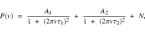(1)

Assuming the same behaviour for solar-like stars, Eq. (1) was fitted to the mean PWTs above $4.0 \times 10^{-5}$ Hz of our four spectral-type stars. To perform these non-linear fits, the Marquardt method was applied (Press et al. 1986). The fitted range covers from $4.0 \times 10^{-5}$ to $2.5 \times 10^{-3}$ Hz, because at lower frequencies, the data are filtered, which is the reason it is not possible to conclude anything about super-granulation or long-period convective movements. However, this non-linear fit is not robust enough to appropriately modify the initial guesses for the lifetime parameters $\tau$ ; so, with a "wrong'' value of these parameters, the fit just does not converge. However, when using a value that allows the fit to converge, the A parameters are very robust and it works very well even with initial guesses far from the final values. For this reason, contrary to the values for A, the parameters $\tau _{1}$ and $\tau_{2}$ were not obtained directly from the fit, but estimated beforehand as a first step of an iterative process.

In order to estimate the initial guesses of the lifetimes well, the fits of the stellar PWTs were done iteratively in a double loop, where $\tau_{2}$ took values between 12 and 48 h with 2 h steps, and for each value of $\tau_{2}$ , $\tau _{1}$ took values between 200 and 700 s with 20 s steps. The idea was to find the values of $\tau_{2}$ and $\tau _{1}$ that minimise the $\chi^{2}$ of the non-linear fit. It was found that the value for $\tau_{2}$ is not critical in the range where the fit was made (above $4.0 \times 10^{-5}$ Hz), and a value of 28 h works fairly well. Further, using this value for $\tau_{2}$ , a first estimation for $\tau _{1}$ is obtained from the minimisation of $\chi^{2}$ .

$\begin{figure} \par\includegraphics[width=7cm,clip]{3620fig4.ps} \end{figure}$	Figure 4: Mean weighted average PWTs in logarithmic scale for the analysed F stars (continuous line) and for the generated power spectrum (dotted line) above $4.0 \times 10^{-5}$ Hz, where the data are not filtered.
Open with DEXTER

Table 5: Parameters A₁ (in arbitrary units) and $\tau _{1}$ (in seconds), related to the granular contrast and its characteristic lifetime, obtained from the weighted average PWTs.

With these values for $\tau_{2}$ , and $\tau _{1}$ and the fitted values for A₁, A₂ and N, numerical power spectra are generated for each analysed spectral type using Eq. (1). The created power spectrum for the F stars is plotted in Fig. 4, showing that it is possible to reproduce the observed PWTs of the stars with the two functions given in Eq. (1), with characteristic lifetimes $\tau_{1} \simeq 9$ min and $\tau_{2} \simeq 28$ h, plus noise. In Fig. 4, $\tau _{1}$ has a value of 500 s and $\tau_{2}$ of 100 800 s, and the parameters A₁, A₂, and N were obtained from the fit to the PWTs of the analysed F stars.

To obtain a better estimation of $\tau _{1}$ , the linear fits used in Sect. 3.1 were performed on the generated power spectrum of each spectral type, and the value of $\tau _{1}$ was changed slightly till the slopes of these fits were equal to the observed ones for each spectral type. Changes in $\tau_{2}$ did not affect the values of the fitted slopes and the parameters A₁, A₂, and N were recalculated from the non-linear fit to Eq. (1) for each value of $\tau _{1}$ used.

The results obtained for the parameters A₁ and $\tau _{1}$ , related to the contrast and characteristic time scale for granulation, are shown in Table 5. A clear change appears in both parameters, increasing from F to M stars. As the WT was not calibrated in amplitude, parameter A₁ has arbitrary units.

4 Analysis of a G type star: the Sun

The data used in this section correspond to solar observations with the SPM-VIRGO experiment. This irradiance data are obtained from three sun-photometers that are part of the SPM-VIRGO experiment (Fröhlich et al. 1995) aboard the SOHO satellite. Data are simultaneously obtained at three wavelengths: 402 nm (B), 500 nm (G), and 865 nm (R) at a cadence of exactly 60 s. The data have a filter at low frequency, below $\approx$ 5 days.

$\begin{figure} \par\includegraphics[width=7cm,clip]{3620fig5.ps} \end{figure}$	Figure 5: PWTs in logarithmic scale for 480 days of solar VIRGO data in the blue channel, at the maximum of the solar activity (continuous line) and at the minimum (dotted line).
Open with DEXTER

$\begin{figure} \par\includegraphics[width=7cm,clip]{3620fig6.ps} \end{figure}$	Figure 6: PWTs in logarithmic scale for 480 days of solar VIRGO data in the three channels (B, G, R) at the maximum of the solar activity.
Open with DEXTER

From the full data series, series of 480 and 54 days with a cadence of 120 s at the maximum and minimum of solar activity were selected, in the three available filters. The series of 480 days are the longest possible series at maximum and minimum, and they were used to analyse the behaviour of the solar convective structures at maximum and minimum of solar activity. The series of 54 days were used to be directly comparable with our stellar observed data.

For the series of 480 days of data, a WT was calculated with the same "mother wavelet'' and number of scales used with the stellar data. The PWT for filter B at maximum and minimum of the solar activity are plotted in Fig. 5, and the PWT for the three filters at the Maximum of the Solar Activity are shown in Fig. 6.

The series of 54 days were analysed following the same procedure as the stellar data. First, the window of the stellar observed data was applied to these solar series; second, the mean values of each day of data was removed and the PWT obtained. The slopes of the linear fits to the PWTs of the series of 480 days of data in the same ranges where the stellar data were fitted are shown in Table 6, and Table 7 shows the results for the series of 54 days.

4.1 The lifetimes

The solar data were reproduced as the stellar data with Eq. (1), which means the assumption of only two convective structures present in the Sun. To reproduce the slopes of Table 6, values of $\tau_{1}=210$ s and $\tau_{2}=28$ h are needed. As can be seen in Table 6, a consistently slight decrease in the slopes exists between the slopes fitted at maximum and minimum of solar activity, but well within the errors of the fits.

This value of $\tau _{1}$ needed to reproduce the observed slopes of the linear fits to the PWTs of the solar data is smaller than the ones needed to reproduce the slopes of the stellar PWTs, although we expect to have similar values, at least for G stars.

The biggest difference between the solar and the stellar data, after the solar data were analysed with the same length, cadence, and windows function as the stellar ones is the terrestrial atmospheric noise present in the stellar but not in the solar data. To see if this noise could produce the obtained difference in the slopes of the linear fits, random noise was added to the time solar series of data at a level that allowed us to reproduce the slopes of the linear fits to the logarithm of the PWTs of the stellar data in the range from $0.7 \times 10^{-3}$ to $2.5 \times 10^{-3}$ Hz. However, the slopes in the range from $1.0 \times 10^{-4}$ to $0.6 \times 10^{-3}$ Hz did not change within the errors, although a slight increase was obtained.

Table 6: Slopes of the linear fits to the logarithm of the PWTs of the solar series for 480 days of data.

Table 7: Slopes of the linear fits to the logarithm of the PWTs of the solar series for 54 days of data analysed as the stellar data, including its observed window function.

The characteristic lifetime of 210 s found for the solar granulation, even though shorter than most of the values found in the literature (Hirzberger et al. 1999), is not incompatible with some of them (Title et al. 1989), and it fully agrees with the latest results obtained by Del Moro (2004). However, this value is clearly smaller than the one found for G type stars, even when the solar data were analysed matching the stellar data, that is, by using the same length of data, the window function, and with random noise introduced to simulate the effect of the terrestrial atmosphere. Related to this difference, it is very interesting to note the recent work of Bruntt et al. (2005) where the acoustic power spectrum of Procyon A (F5) is analysed with a result for the granulation timescale of $750 \pm 200$ s.

It is interesting to compare the result of the characteristic lifetime of the solar granulation found here with previous estimations obtained in our past work, from the analysis of the solar power spectrum. The first result (Jiménez et al. 1988) from ground based radial velocity data, gives a value of $\tau=300$ s. A more recent work (Vázquez Ramió et al. 2002), where the same data used in this paper were analysed using FFT's instead of WT's, produces results fully compatible with ours, being $\tau \sim 220$ s with a slight variation depending on the used filter. However, data in radial velocity instead of irradiance (Régulo et al. 2002) taken from GOLF (Gabriel et al. 1995) aboard SOHO simultaneously with the irradiance data used in this work, gives results similar to the ones obtained here for G type stars, $\tau=585$ s in the maximum of solar activity and $\tau=463$ s in the minimum.

4.2 The contrast

To fit the contrast of the convective structures A₁ and A₂ in Eq. (1), the values of $\tau_{1}=210$ s and $\tau_{2}=28$ h obtained previously to reproduce the slopes of Table 6, were used. With these values of $\tau$ , the non-linear fit to Eq. (1) was performed up to 36 h and the values of the contrast of the convective structures A₁ and A₂ were calculated for the three filters providing the already known evidence for variations in the convective contrast which increases towards shorter wavelengths, see Fig. 6. Moreover, a clear decrease in the contrast around 50 % for the Blue and Green filters and near 30% for the Red one, were obtained from maximum to minimum in the convective structure with $\tau=28$ h that represents the super-granulation range, see Table 8. Although some part of this change could be due to the change from maximum to minimum of the active regions, as this region of the spectrum was filtered and the fits were made till 36 h only, it is difficult to assume that all the change is a remainder of changes in the very low frequency part of the spectrum.

Table 8: Ratios of the parameters A₁ (obtained at maximum and minimum of the solar activity) and A₂. These parameters are related with the granular and super-granulation contrast, obtained from a non-linear fit of Eq. (1) to the solar PWTs.

As far as the granulation contrast variation from maximum to minimum solar activity, our analysis do not provide conclusive evidence, although values are consistently below unity (see Table 8) they lie well within errors. However, it is important to point out that the quality of VIRGO solar data allows a much more precise analysis than the one performed in this work, where the aim was to carry out an analysis to be compared with the stellar data. Nevertheless, even with this limited analysis, the results are fully compatible with more precise studies that have been done previously (Vázquez Ramió et al. 2002).

5 Discussion and conclusions

Weighted average WT of MS stars with spectral type F, G, K, and M have been analysed in this paper to look for changes in the convective structures of these stars with the spectral type. Due to the window function of the observed stars, only information above $4.0 \times 10^{-5}$ Hz is useful; for this reason we concentrated on the possible changes in the granulation structures.

Two linear fits at frequency intervals above $1.0 \times 10^{-4}$ Hz were performed where their slopes are related to the lifetime of the granulation. A clear increase in these slopes towards cooler stars was found. The slopes of stars with spectral type G depart from the general tendency, because these stars are the faintest of the sample and, especially in the range between $0.7 \times 10^{-3}$ and $2.5 \times 10^{-3}$ Hz, the random noise effects tend to diminish the slope of the faintest stars and to increase the slope of the brightest, which in our sample are the stars with spectral type K.

When using a model for the PWTs as the sum of two functions, as shown in Eq. (1) with characteristic times $\tau _{1}$ around 9 min and $\tau_{2}$ of 28 h plus random noise, values of $\tau _{1}$ between 500 and 620 s are required, with $\tau_{1}=500$ s the value that allows to reproduce the slopes of the linear fits to the logarithm of the PWT of F stars and $\tau_{1}=620$ s, the value needed for M stars. This means a change of 20% in the characteristic lifetime of the granulation with the spectral type, in the sense that the lifetime is slightly higher for cooler stars.

The mean PWTs of each spectral type were fitted to Eq. (1) in order to analyse how the granulation contrast changes with the spectral type. The results show that the granulation contrast increases about 30% on average from one spectral type to the next cooler one. We could think that this change in the contrast is partially due to the different magnitude distribution of the different spectral types; however, this distribution is not linear with spectral type, as the G and K stars are the dimmest and brightest, respectively, while the contrast increases steadily from F to M stars.

It seems clear from our analysis, given the error bars, that the characteristic parameters of the granulation, contrast and lifetime, increase with the spectral type for late type stars. Such increase is higher for the contrast parameter. On the other hand, stellar evolution theory predicts an increase in the depth of the convective envelopes towards cooler stars (Kippenhahn & Weigert 1991). Thus, it is not surprising to find that the lifetime and the contrast of the granulation are bigger when the convective zone is deeper.

Related to the change of solar convective parameters with the activity cycle, a slight decrease in the granulation lifetime from maximum to minimum is found, although within the errors, as well as a clear change in the contrast for the super-granulation decreasing with activity. No changes in the granulation contrast with solar activity is observed.

An observational approach to convection in main sequence stars

1 Introduction