A&A 443, 451-463 (2005)
DOI: 10.1051/0004-6361:20041903
P. Favre1,2 - T. J.-L. Courvoisier1,2 - S. Paltani1,3
1 - INTEGRAL Science Data Center, 16 Ch. d'Ecogia, 1290
Versoix, Switzerland
2 - Geneva Observatory, 51 Ch. des
Maillettes, 1290 Sauverny, Switzerland
3 - Laboratoire
d'Astrophysique de Marseille, Traverse du Siphon, BP 8, 13376
Marseille Cedex 12, France
Received 25 August 2004 / Accepted 3 August 2005
Abstract
We analyse the ultraviolet variability time scales
in a sample of 15 type 1 Active Galactic Nuclei (AGN) observed by
IUE. Using a structure function analysis, we demonstrate the
existence in most objects of a maximum variability
time scale of the order of 0.02-1.00 year. We do not find any
significant dependence of these maximum variability time scales on
the wavelength, but we observe a weak correlation
with the average luminosity of the objects. We also observe
in several objects the existence of long-term variability, which
seems decoupled from the short-term one. We interpret the
existence of a maximum variability time scale as a possible
evidence that the light curves of type 1 AGN are the result of
the superimposition of independent events. In the framework of
the so-called discrete-event model, we study the event energy and
event rate as a function of the object properties. We
confront our results to predictions from existing models
based on discrete events. We show that models based on a fixed
event energy, like supernova explosions, can be
ruled out. In their present form, models based on magnetic
blobs are also unable to account for the observed relations. Stellar
collision models, while not completely satisfactory, cannot be excluded.
Key words: galaxies: active - galaxies: Seyfert - quasars: general - ultraviolet: galaxies
This difficulty led several authors (Cid Fernandes et al. 1996; Paltani & Courvoisier 1997 (hereafter PC97); Aretxaga et al. 1997; Cid Fernandes et al. 2000 (hereafter CSV00); see also Aretxaga & Terlevich 1994) to consider a more phenomenological approach based on the discrete-event model, which provides a simple explanation for the variability: The variability is the result of a superimposition of independent events occurring at random epochs at a given rate. The motivations for the discrete-event model are twofold: Temporal analysis allows to constrain the event properties, while its generality leaves room for a large variety of physical events. It can be a reasonable approximation for models like starburst (Aretxaga & Terlevich 1994; Aretxaga et al. 1997), stellarcollisions (Courvoisier et al. 1996; Torricelli-Ciamponi et al. 2000), or magnetic blobs above an accretion disk (Haardt et al. 1994).
In this paper, we use data from the International Ultraviolet Explorer (IUE) covering about 17 years to determine the UV characteristic time scales in a sample of Seyfert 1 galaxies and QSOs, using a methodology similar to that used in Collier & Peterson (2001, hereafter CP01). While CP01 concentrated on the measure of time scales shorter than 100 days by selecting short portions of the light curves in which the time sampling was denser, we use here the full available light curves (on average 16.5 years), highlighting a wider range of time scales, and extend the sample to 15 objects. Furthermore, using 12 wavelength windows between 1300 and 3000 Å, we investigate for the first time the existence of a wavelength dependence of the variability time scale.
We interpret the variability properties of our objects in terms of discrete-event model, and we study their parameters as a function of the object properties. Our approach is similar to that of CSV00, although we use data from IUE gathered during almost 17 years, while they use optical data covering about seven years. Furthermore, the sample of CSV00 is composed of PG quasars (median z: 0.16) while ours is mainly composed of Seyfert 1 galaxies at a much smaller redshift (median z: 0.033). Their observations thus not only cover about three times less time than ours, but the observation durations arefurther diminished in the observer's frame. Finally, as variability increases towards shorter wavelengths (Kinney et al. 1991; Paltani & Courvoisier 1994; di Clemente et al. 1996; Trèvese & Vagnetti 2002), the study of the variability is more efficient in the UV than in the optical.
The formalism of the discrete-event model was mainly developed in Cid Fernandes et al. (1996), PC97, Aretxaga et al. (1997), and CSV00. In the discrete-event model, the variability is due to the superimposition of independent events, occurring at random epochs, on top of a possible constant source. In the simplest form that we use here, all events are identical.
The total luminosity density at wavelength ![]() can be expressed as:
can be expressed as:
 |
(1) |
We selected all the type 1 AGN spectra available in early December 2001 in the INES (IUE Newly Extracted Spectra) v3.0 database at VILSPA/LAEFF, which used a new noise model and background determination (Rodríguez-Pascual et al. 1999). We extracted the objects monitored for several years for which at least 20 large aperture, small dispersion observations have been performed with the SWP instrument (1150-1950 Å). These conditions were imposed by the temporal analysis (see Sect. 4.1). Table 1 gives a list of the selected objects with their common names and redshifts. We finally have in our sample 13 Seyfert 1 galaxies, one broad-line radio galaxy (BLRG), and one quasar.
| Name | Classification | z | SWP | LWP/R |
|
EB-V | |
| (year) | (
|
||||||
| Mrk 335 | Seyfert 1 | 0.0257 | 26 | 28 | 12.66 |
|
0.059 |
| Mrk 509 | Seyfert 1 | 0.0343 | 39 | 32 | 15.06 |
|
0.060 |
| Mrk 926 | Seyfert 1 | 0.0475 | 22 | 16 | 14.51 |
|
0.053 |
| Mrk 1095 | Seyfert 1 | 0.0331 | 35 | 23 | 10.82 |
|
0.170 |
| NGC 3516 | Seyfert 1 | 0.0088 | 71 | 22 | 16.67 |
|
0.054 |
| NGC 3783 | Seyfert 1 | 0.0097 | 95 | 84 | 13.54 |
|
0.141 |
| NGC 4151 | Seyfert 1 | 0.0033 | 153 | 137 | 18.09 |
|
0.031 |
| NGC 4593 | Seyfert 1 | 0.0083 | 20 | 15 | 8.31 |
|
0.034 |
| NGC 5548 | Seyfert 1 | 0.0171 | 175 | 148 | 16.60 |
|
0.024 |
| NGC 7469 | Seyfert 1 | 0.0163 | 65 | 15 | 17.79 |
|
0.079 |
| 3C 120.0 | Seyfert 1 | 0.0330 | 43 | 21 | 15.40 |
|
0.160 |
| 3C 273 | Quasar | 0.1583 | 124 | 114 | 15.36 |
|
0.027 |
| 3C 390.3 | BLRG | 0.0561 | 99 | 11 | 16.37 |
|
0.071 |
| Fairall 9 | Seyfert 1 | 0.0461 | 139 | 63 | 15.80 |
|
0.042 |
| ESO 141-55 | Seyfert 1 | 0.0371 | 26 | 16 | 11.33 |
|
0.075 |
![\begin{figure}
\par\includegraphics[width=8.8cm,clip]{1903f1.eps}\end{figure}](/articles/aa/full/2005/44/aa1903-04/img49.gif) |
Figure 1: Average IUE spectrum of the Seyfert 1 galaxy Mrk 335. The position of the 12 spectral windows is indicated by the gray areas. |
When building the light curves, FITS headers of all spectra
were carefully checked for anomalies. We excluded spectra which were affected by
an objective technical problem stated in the FITS headers (e.g., no
significant flux detected, object out of aperture, no guiding, no
tracking). Spectra for which the pointing direction was
farther than 10
![]() from the object position were also discarded. For 3C 273,
the selected spectra correspond to the list described in Türler et al. (1999).
from the object position were also discarded. For 3C 273,
the selected spectra correspond to the list described in Türler et al. (1999).
Two observations showing clearly spurious fluxes were removed; one in NGC 3516 (Julian day: 2 449 760.78), and one in NGC 5548 (Julian day: 2 448 993.89). No correction for reddening was applied, as this should have no qualitative influence on our results (See Sect. 5.3).
The light curves at 1300-1350 Å for all objects in our sample are presented in Fig. 2. The monitoring durations in the rest frame of the objects are between 8.31 years (NGC 4593) and 18.09 years (NGC 4151), see Table 1.
![\begin{figure}
\par\includegraphics[width=16.7cm,clip]{1903f2.eps}\end{figure}](/articles/aa/full/2005/44/aa1903-04/img51.gif) |
Figure 2: Light curves in the range 1300-1350 Å for the 15 objects of our sample. Only one error bar is drawn on each panel for clarity (in the upper- or lower-left corner). |
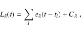
The first-order structure function of a light curve x(t) is a
function of the time lag ![]() ,
and is defined by:
,
and is defined by:
 |
(6) |
We estimate the SFs of our light curves by averaging flux differences
over predefined time bins, considering only the bins containing at least six pairs. We oversample
the SFs (i.e. the bin-to-bin interval is smaller than the bin width) in order to emphasize
their characteristics. The bins are geometrically spaced, i.e. the bin-to-bin interval is
constant on a Log scale.
Finally, we do not attempt to determine error bars on the
SFs, as none of the prescriptions found in the literature
seem satisfactory. For example, in the prescriptions of
Simonetti et al. (1985) and CP01, the uncertainty on the SF values is proportional to
ni -1/2, where
ni is the number of pairs in bin i. These prescriptions produce underestimated error bars at
large ![]() (illustrated in
Fig. 3 of CP01), because the number of pairs is increasing roughly exponentially with
(illustrated in
Fig. 3 of CP01), because the number of pairs is increasing roughly exponentially with ![]() because
of the geometric spacing of the bins, while
the total information in the light curve is finite.
because
of the geometric spacing of the bins, while
the total information in the light curve is finite.
Structure functions of the 1300-1350 Å light curves for the 15 objects of our sample are presented in Fig. 3. The asymptotic values at twice the light curve variances are also shown. Narrow structures in the SF (see e.g. Fairall 9, 3C 390.3) are very probably due to the high inter-correlation of the SF (because the same measurements are used in several bins), and are probably not physical.
![\begin{figure}
\par\includegraphics[width=17cm,clip]{1903f3.eps}\end{figure}](/articles/aa/full/2005/44/aa1903-04/img56.gif) |
Figure 3:
Structure functions of the light curves at 1300-1350 Å. The
horizontal dashed lines show the asymptotic value of twice the
variance of x(t). The continuous line shows the best fit, while the value of
|
In Fig. 3, we observe that, for a majority of objects, the SFs show a plateau at about twice the variance of the light curves.
However, in some cases, the SF continues to increase for ![]() larger than
larger than ![]() 5 years.
Paltani et al. (1998) presented a similar analysis on 3C 273, and
concluded that a second component, varying on
long time scales, was present, particularly at long wavelengths. Such a component
appears in the form of a SF rising sharply at large
5 years.
Paltani et al. (1998) presented a similar analysis on 3C 273, and
concluded that a second component, varying on
long time scales, was present, particularly at long wavelengths. Such a component
appears in the form of a SF rising sharply at large ![]() .
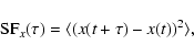
To cope with the possibility of the existence of a second
component, we fit the SFs using the same function as in Paltani et al. (1998):
.
To cope with the possibility of the existence of a second
component, we fit the SFs using the same function as in Paltani et al. (1998):
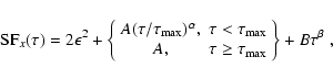 |
(7) |
We first fit the 1300-1350 Å SFs; we shall discuss the longer wavelength SFs
in Sect. 4.3. The values of
![]() are given in Table 2, corrected for time dilatation. The best fits are shown in
Fig. 3 by a continuous line.
are given in Table 2, corrected for time dilatation. The best fits are shown in
Fig. 3 by a continuous line. ![]() was fitted as a free parameter. The best fit values found for these parameters
were comparable to the noise variance mesured in the light curves.
In four objects (NGC 3516, NGC 4151, NGC 7469,
Fairall 9), the fit does not converge unless we fix the noise
parameter
was fitted as a free parameter. The best fit values found for these parameters
were comparable to the noise variance mesured in the light curves.
In four objects (NGC 3516, NGC 4151, NGC 7469,
Fairall 9), the fit does not converge unless we fix the noise
parameter ![]() and the slope
and the slope ![]() in the fits. We have
tested that reasonable choices of
in the fits. We have
tested that reasonable choices of ![]() and
and ![]() have little influence on
the value of
have little influence on
the value of
![]() in those four SFs.
We checked as well that the monitoring duration (
in those four SFs.
We checked as well that the monitoring duration (![]() in Table 1) had no influence on the measure
of
in Table 1) had no influence on the measure
of
![]() .
.
The SFs of NGC 3516, and NGC 4151 show strong structures between 0.1 and 1 year,
but their behavior at ![]() is compatible with an extrapolation of their behavior at
is compatible with an extrapolation of their behavior at ![]() .
Our fit interprets the strong structures as evidence of a
.
Our fit interprets the strong structures as evidence of a
![]() ,
but we need to check
that the structures themselves do not result from the sampling. To do that, we simulated light curves using a random
walk, and projected them on the original light curve sampling. None of our simulations reproduced the
observed structures in the SFs, and we consider therefore that a maximum time scale is really present in
these two objects. The shape of the SFs forces us however to make the error bars on
,
but we need to check
that the structures themselves do not result from the sampling. To do that, we simulated light curves using a random
walk, and projected them on the original light curve sampling. None of our simulations reproduced the
observed structures in the SFs, and we consider therefore that a maximum time scale is really present in
these two objects. The shape of the SFs forces us however to make the error bars on
![]() extend up to 1 year in these two objects. In Fairall 9, no plateau can be seen, but there is a clear change in the slope
of the SF between
extend up to 1 year in these two objects. In Fairall 9, no plateau can be seen, but there is a clear change in the slope
of the SF between ![]() year and
year and ![]() years. We interpret this as the presence of a
years. We interpret this as the presence of a
![]() in this range of time scale, followed by a very strong slowly varying component.
In NGC 3783, a similar change of slope occurs, and it is impossible to locate
in this range of time scale, followed by a very strong slowly varying component.
In NGC 3783, a similar change of slope occurs, and it is impossible to locate
![]() unequivocally. This is reflected in the error bar on
unequivocally. This is reflected in the error bar on
![]() for this object. Several other objects
show the existence of a second variability component, but it does not affect the measurement of
for this object. Several other objects
show the existence of a second variability component, but it does not affect the measurement of
![]() .
.
We repeated the analysis of the SFs without including a slow component of variability in the model, i.e. we fitted the data with B=0. The values
of
![]() found are compared in Table 2. The values found with B=0 are all inside the error
bars except for NGC 3516, NGC 3783 and NGC 4151. For NGC 3516 and NGC 4151, the fits do not represent the data.
Thus for a majority of objects, the addition of a second component has no effect while it significantly improves the fits
for NGC 3516, NGC 3783 and NGC 4151.
found are compared in Table 2. The values found with B=0 are all inside the error
bars except for NGC 3516, NGC 3783 and NGC 4151. For NGC 3516 and NGC 4151, the fits do not represent the data.
Thus for a majority of objects, the addition of a second component has no effect while it significantly improves the fits
for NGC 3516, NGC 3783 and NGC 4151.
We conclude that with these data, we cannot decide if a second component is detected or not. This second variability component, while interesting per se, is outside the scope of this paper, and shall not be discussed further.
For all the objects, we estimate the effect of the binning on
![]() by computing and
fitting 100 SFs (at 1300-1350 Å) for
each object with different binnings, with corresponding bin-to-bin intervals between 0.002 year and 0.1 year.
For all objects, the distribution of the measured
by computing and
fitting 100 SFs (at 1300-1350 Å) for
each object with different binnings, with corresponding bin-to-bin intervals between 0.002 year and 0.1 year.
For all objects, the distribution of the measured
![]() is
mono-peaked, meaning that a single value of
is
mono-peaked, meaning that a single value of
![]() was
always found by the algorithm. The width of this peak determines an
empirical uncertainty on
was
always found by the algorithm. The width of this peak determines an
empirical uncertainty on
![]() (Table 2).
(Table 2).
We measure
![]() from 0.022 to 0.997 year for the 15 objects
of our sample. Our time scales are of the same order of magnitude as
the one found by previous studies in the optical-UV (Hook et al. 1994; Trevese et al. 1994; Cristiani et al. 1996; Paltani et al. 1998; Giveon et al. 1999; CSV00). The time scales
found by CP01 and Paltani et al. (1998) are indicated in Fig. 3 by a vertical
line and are in reasonable agreement with what we have found, 3C 390.3 and
NGC 3783 excepted. The discrepancy can be explained by the fact that CP01 "detrend'' their
SFs with a linear component (i.e. they remove a
linear fit from their light curves), arguing that the measured SF will
deviate from their theoretical shape if the light curve shows a linear
trend. Our method of including a second, slowly variable component in
the structure functions is more general than the "detrending'', because it makes
less strict assumptions on
the temporal properties of the slowly varying component.
It is nevertheless equivalent in the case where a linear trend is
effectively present in the data. Our method is also more
consistent in the sense that all components are handled in a similar
way. Furthermore, a linear trend would make little sense in
objects like NGC 4151.
from 0.022 to 0.997 year for the 15 objects
of our sample. Our time scales are of the same order of magnitude as
the one found by previous studies in the optical-UV (Hook et al. 1994; Trevese et al. 1994; Cristiani et al. 1996; Paltani et al. 1998; Giveon et al. 1999; CSV00). The time scales
found by CP01 and Paltani et al. (1998) are indicated in Fig. 3 by a vertical
line and are in reasonable agreement with what we have found, 3C 390.3 and
NGC 3783 excepted. The discrepancy can be explained by the fact that CP01 "detrend'' their
SFs with a linear component (i.e. they remove a
linear fit from their light curves), arguing that the measured SF will
deviate from their theoretical shape if the light curve shows a linear
trend. Our method of including a second, slowly variable component in
the structure functions is more general than the "detrending'', because it makes
less strict assumptions on
the temporal properties of the slowly varying component.
It is nevertheless equivalent in the case where a linear trend is
effectively present in the data. Our method is also more
consistent in the sense that all components are handled in a similar
way. Furthermore, a linear trend would make little sense in
objects like NGC 4151.
| Object |
|
|
|
| (year) | (year) | (year) | |
| Mrk 335 |
|
0.222 |
|
| Mrk 509 |
|
0.550 |
|
| Mrk 926 |
|
0.227 |
|
| Mrk 1095 |
|
0.438 |
|
| NGC 3516 |
|
4.896 |
|
| NGC 3783 |
|
1.229 |
|
| NGC 4151 |
|
2.200 |
|
| NGC 4593 |
|
0.262 |
|
| NGC 5548 |
|
0.154 |
|
| NGC 7469 |
|
0.023 |
|
| 3C 120.0 |
|
0.287 |
|
| 3C 273 |
|
0.459 |
|
| 3C 390.3 |
|
0.635 |
|
| Fairall 9 |
|
0.760 |
|
| ESO 141-55 |
|
1.014 |
|
An easy way to explain the existence of a maximum variability time scale is provided by the discrete-event model.
For a Poissonian sequence of events, the SF is proportional to the SF of a single event (Paltani 1996; Aretxaga et al. 1997; CSV00)
and only has structures on time scales shorter than the event duration.
We interpret the observed SFs using discrete events for which we assume a triangular, symmetric shape.
The event shape was chosen for its simplicity (Paltani et al. 1998), but it
has been shown that choosing other shapes does not affect
significantly the results given by the temporal analysis (CSV00).
Our events are described with only two parameters at wavelength ![]() :
the event amplitude
:
the event amplitude
![]() and the event duration
and the event duration
![]() ;
;
![]() being defined as the time
needed to reach the maximum flux.
It follows that
being defined as the time
needed to reach the maximum flux.
It follows that
![]() and
and
![]() in this case (see Sect. 2).
in this case (see Sect. 2).
While the SFs are in theory able to measure the event duration, this measure can be affected by
the noise and sampling of the light curve in a complex and unpredictable way. To test if
![]() measures a property of the
light curves, and not of the sampling, we produce synthetic light curves
by simulation, and measure their
measures a property of the
light curves, and not of the sampling, we produce synthetic light curves
by simulation, and measure their
![]() .
In the simulations, we add randomly triangular events with a
given duration
.
In the simulations, we add randomly triangular events with a
given duration
![]() ,
keeping the same sampling as the
original light curve.
A noise with an amplitude equal to the average of the instrumental noise is added to each light curve.
We take 40 test values for
,
keeping the same sampling as the
original light curve.
A noise with an amplitude equal to the average of the instrumental noise is added to each light curve.
We take 40 test values for
![]() ,
from
10-3 to 10 years, geometrically spaced.
,
from
10-3 to 10 years, geometrically spaced.
For each object and each
![]() ,
we build 1000 light curves, compute
their SFs and, measure
,
we build 1000 light curves, compute
their SFs and, measure
![]() using the
method described above. The event rate N is randomly chosen between 5
and 500 events per year.
The result of the simulation is, for each object and each
using the
method described above. The event rate N is randomly chosen between 5
and 500 events per year.
The result of the simulation is, for each object and each
![]() ,
the distribution of the
resulting
,
the distribution of the
resulting
![]() .
These distributions allow us to determine which input
.
These distributions allow us to determine which input
![]() can provide
the observed
can provide
the observed
![]() .
For 3C 273 for example, the distribution of
.
For 3C 273 for example, the distribution of
![]() produced
a peak around 0.56 year, as represented in Fig. 4. The fit of the peak of Fig. 4 with a Gaussian
gives
produced
a peak around 0.56 year, as represented in Fig. 4. The fit of the peak of Fig. 4 with a Gaussian
gives
![]() years.
years.
We note that we never observe a B parameter (see Sect. 4.1) significantly larger than 0 in our simulations. This is expected as we do not include a second component.
The simulations for all objects showed a result qualitatively identical to that for 3C 273, i.e. the distributions
of
![]() present a single peak. This means therefore that, for each object,
present a single peak. This means therefore that, for each object,
![]() determines a unique event duration, that can be derived from the simulations. The values of
determines a unique event duration, that can be derived from the simulations. The values of
![]() are
given in Table 2. We stress that our simulations are driven by the real sampling of the light curves,
and are therefore more specific than, for example, those discussed in Welsh (1999), or CP01.
are
given in Table 2. We stress that our simulations are driven by the real sampling of the light curves,
and are therefore more specific than, for example, those discussed in Welsh (1999), or CP01.
For each object of the sample, we apply the method described in Sect. 4.1 to compute the event durations from the light curves 1450 to 2975 Å.
Structure functions from 1300 Å to 3000 Å are presented in Appendix A for each object, along with a description of the particularity of each set of SFs. As an example, we show the case of NGC 5548 in Fig. 5.
It is not possible to deduce a value of
![]() for all 180 light curves. This is mainly due to the fact that, for some of the objects, the number of
observations in the LW range is too small. In addition some particular light curves are very noisy. In such cases,
the SF usually does not have the canonical shape, and the fit does not succeed. We thus reject the time scale corresponding to those
particular SFs. Each individual case is described in Appendix A. In some cases, the noise is such that, although
for all 180 light curves. This is mainly due to the fact that, for some of the objects, the number of
observations in the LW range is too small. In addition some particular light curves are very noisy. In such cases,
the SF usually does not have the canonical shape, and the fit does not succeed. We thus reject the time scale corresponding to those
particular SFs. Each individual case is described in Appendix A. In some cases, the noise is such that, although
![]() can be derived from the SF, its
uncertainty is very large. In such cases, one should interpret any variation in
can be derived from the SF, its
uncertainty is very large. In such cases, one should interpret any variation in
![]() with caution.
with caution.
Figure 6 presents the variability time scale
![]() as
a function of the wavelength for all the objects. We find that
as
a function of the wavelength for all the objects. We find that
![]() is reasonably
constant over the wavelength range we use, as the small fluctuations
can be explained by the difficulty to measure a precise
value of
is reasonably
constant over the wavelength range we use, as the small fluctuations
can be explained by the difficulty to measure a precise
value of
![]() on some noisy SF. For the particular case of
NGC 5548 for example, the variations are inside the uncertainties derived in the previous section.
This result was a also found by Paltani et al. (1998) for 3C 273.
on some noisy SF. For the particular case of
NGC 5548 for example, the variations are inside the uncertainties derived in the previous section.
This result was a also found by Paltani et al. (1998) for 3C 273.
In two objects however, NGC 7469 and Fairall 9, the SFs present a very strong
increase in
![]() at long wavelengths. For NGC 7469, this is due to a lack of short
term sampling of the LW light curves, which prevents the recovery of any time scale below 0.5 year. In Fairall 9, a similar lack
of short term sampling affects the determination of
at long wavelengths. For NGC 7469, this is due to a lack of short
term sampling of the LW light curves, which prevents the recovery of any time scale below 0.5 year. In Fairall 9, a similar lack
of short term sampling affects the determination of
![]() .
However, the values of
.
However, the values of
![]() in the LW range
are within the uncertainties on
in the LW range
are within the uncertainties on
![]() determined at 1300 Å.
determined at 1300 Å.
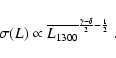
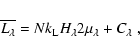
The relationship between the event duration and the luminosity has some important consequences for the discrete-event model that we will discuss below (Sect. 5.4). We note, however, that only a weak dependence between the event duration and the average luminosity of the object is possible as the values of the former cover less than two orders of magnitude while the latter covers four orders of magnitude. We thus measure a physical time scale which has at most a small dependence on the luminosity of the objects.
The event duration
![]() as a function of the
average luminosity
as a function of the
average luminosity
![]() of the object at 1300-1350 Å is shown in
Fig. 7. We use a simple cosmology with H0=60 km s-1 Mpc-1, and q0=0.5
throughout.
of the object at 1300-1350 Å is shown in
Fig. 7. We use a simple cosmology with H0=60 km s-1 Mpc-1, and q0=0.5
throughout.
Using Spearman's correlation coefficient, we find a correlation between the event duration and the
luminosity (s=0.38), marginally significant at the 16% level (Null hypothesis). The dependence of
![]() on
on
![]() can be expressed as
can be expressed as
![]() ,
where the index
,
where the index
![]() has been determined using the BCES linear regressions (Akritas & Bershady 1996).
has been determined using the BCES linear regressions (Akritas & Bershady 1996).
![\begin{figure}
\par\includegraphics[width=8.8cm,clip]{1903f7.eps}\end{figure}](/articles/aa/full/2005/44/aa1903-04/img105.gif) |
Figure 7:
Variability time scales
|
The steady component
![]() (Sect. 2)
can have various physical origins. For example, it can be associated to
the non-flaring part of the accretion disk, or to the host-galaxy stellar contribution
(Cid Fernandes et al. 1996; CSV00). We shall however continue our
discussion in a model-independent way.
We can constrain
(Sect. 2)
can have various physical origins. For example, it can be associated to
the non-flaring part of the accretion disk, or to the host-galaxy stellar contribution
(Cid Fernandes et al. 1996; CSV00). We shall however continue our
discussion in a model-independent way.
We can constrain
![]() for a particular light curve by imposing that it does not exceed
the minimum observed luminosity
for a particular light curve by imposing that it does not exceed
the minimum observed luminosity
![]() .
On the other hand,
.
On the other hand,
![]() is an obvious lower limit (although Paltani & Walter (1996)
argued that
is an obvious lower limit (although Paltani & Walter (1996)
argued that
![]() ,
at least for
,
at least for
![]() Å). In the following, we shall use these
two constraints as limiting cases.
Å). In the following, we shall use these
two constraints as limiting cases.
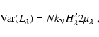
For each object, we compute the event amplitude
![]() from Eq. (5)
using both
from Eq. (5)
using both
![]() and
and
![]() .
Figure 8 shows the
spectral shape of
.
Figure 8 shows the
spectral shape of
![]() for NGC 5548.
We integrate
for NGC 5548.
We integrate
![]() interpolated over the wavelength range 1300-3000 Å
to obtain the energy E released in one event, assuming isotropic emission:
interpolated over the wavelength range 1300-3000 Å
to obtain the energy E released in one event, assuming isotropic emission:
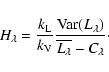
Table 3 gives the event energies and rates found with the
![]() ,
and
,
and
![]() assumptions. Event energies are
found in the range
1048-1052 erg, and maximum event rates in the range
9-1133 event year-1 (
assumptions. Event energies are
found in the range
1048-1052 erg, and maximum event rates in the range
9-1133 event year-1 (
![]() )
while minimum event rates are found in the
range 2-270 event year-1 (upper limit of
)
while minimum event rates are found in the
range 2-270 event year-1 (upper limit of
![]() ).
Fig. 9 shows the event energy E as a function of the 1300-1350 Å luminosity, using the upper
and lower limits on
).
Fig. 9 shows the event energy E as a function of the 1300-1350 Å luminosity, using the upper
and lower limits on
![]() .
.
![\begin{figure}\par\includegraphics[width=8.6cm,clip]{1903f8.eps}\end{figure}](/articles/aa/full/2005/44/aa1903-04/img111.gif) |
Figure 8:
Event amplitude spectrum
|
| Name | N | E | N | E |
| (year-1) | (
|
(year-1) | (
| |
|
|
| |||
| Mrk 335 |
|
|
|
|
| Mrk 509 |
|
|
|
|
| Mrk 926 |
|
|
|
|
| Mrk 1095 |
|
|
|
|
| NGC 3516 |
|
|
|
|
| NGC 3783 |
|
|
|
|
| NGC 4151 |
|
|
|
|
| NGC 4593 |
|
|
|
|
| NGC 5548 |
|
|
|
|
| NGC 7469 |
|
|
|
|
| 3C 120.0 |
|
|
|
|
| 3C 273 |
|
|
|
|
| 3C 390.3 |
|
|
|
|
| Fairall 9 |
|
|
|
|
| ESO 141-55 |
|
|
|
|
![\begin{figure}
\par\includegraphics[bb=20 150 570 500,clip,width=8.8cm,clip]{1903f9.eps}\end{figure}](/articles/aa/full/2005/44/aa1903-04/img172.gif) |
Figure 9:
Event energy as a function of the object luminosity in the hypothesis
|
![\begin{figure}
\par\includegraphics[bb=20 150 570 500,clip,width=8.8cm,clip]{1903f10.eps}\end{figure}](/articles/aa/full/2005/44/aa1903-04/img173.gif) |
Figure 10:
Event rate as a function of the object luminosity in the hypothesis
|
With
![]() ,
E and
,
E and
![]() are clearly correlated (Spearman correlation coefficient: s=0.85), with a Null hypothesis
probability of less than 0.1%. A linear regression gives
are clearly correlated (Spearman correlation coefficient: s=0.85), with a Null hypothesis
probability of less than 0.1%. A linear regression gives
![]() ,
with
,
with
![]() using the BCES method (Akritas & Bershady 1996) (Fig. 9, left panel).
using the BCES method (Akritas & Bershady 1996) (Fig. 9, left panel).
When using
![]() ,
the correlation is preserved (Spearman: s=0.89), with a Null hypothesis probability of less
than 0.1% and an index
,
the correlation is preserved (Spearman: s=0.89), with a Null hypothesis probability of less
than 0.1% and an index
![]() (Fig. 9, right panel).
We note that E and
(Fig. 9, right panel).
We note that E and
![]() are lower limits
since no corrections for reddening were applied. The correlation should be preserved by applying the corrections, as both E and
are lower limits
since no corrections for reddening were applied. The correlation should be preserved by applying the corrections, as both E and
![]() would be scaled
by the same factor. We tested this hypothesis by correcting the light curves for reddening and recomputing the relation
would be scaled
by the same factor. We tested this hypothesis by correcting the light curves for reddening and recomputing the relation
![]() .
The correlation is
preserved (Spearman correlation coefficient: s=0.83) with an index
.
The correlation is
preserved (Spearman correlation coefficient: s=0.83) with an index
![]() for the case
for the case
![]() as well as for the case
as well as for the case
![]() (Spearman correlation coefficient: s=0.84) with an index
(Spearman correlation coefficient: s=0.84) with an index
![]() .
These values are consistent with
the non-dereddened values.
.
These values are consistent with
the non-dereddened values.
The event rates as a function of the object luminosity are given in Fig. 10, for both the upper and lower limits on
![]() .
A non-significant anticorrelation is found in the
.
A non-significant anticorrelation is found in the
![]() case (Spearman's s=-0.12, Null hypothesis probability of 66.64%),
while a marginally significant anticorrelation is found for
case (Spearman's s=-0.12, Null hypothesis probability of 66.64%),
while a marginally significant anticorrelation is found for
![]() (Spearman's s=-0.39, Null hypothesis probability of 15%).
Using the data corrected for reddening, one finds as well a non-significant anticorrelation (Spearman's s=-0.02, Null hypothesis probability of non-correlation
of 93.96%) in the case
(Spearman's s=-0.39, Null hypothesis probability of 15%).
Using the data corrected for reddening, one finds as well a non-significant anticorrelation (Spearman's s=-0.02, Null hypothesis probability of non-correlation
of 93.96%) in the case
![]() ,
and a non-significant anticorrelation for
,
and a non-significant anticorrelation for
![]() (Spearman's s=-0.17, Null hypothesis
probability of 54.12%).
(Spearman's s=-0.17, Null hypothesis
probability of 54.12%).
We showed in Sect. 5.1 that the event
duration
![]() is a shallow function of the luminosity
and in Sect. 5.3 that the measured event energy
is a shallow function of the luminosity
and in Sect. 5.3 that the measured event energy
![]() ,
with
,
with
![]() .
These two results, expectedly, lead to values of
.
These two results, expectedly, lead to values of ![]() in agreement
with the measure of PC97. We thus established that the event parameter
which drives the
in agreement
with the measure of PC97. We thus established that the event parameter
which drives the ![]() dependence is the event energy, and not its duration, nor its rate.
dependence is the event energy, and not its duration, nor its rate.
PC97 showed that in this case one should expect a variability-luminosity relation in the form:
 |
(9) |
We have shown that a characteristic variability time scale exists, which
can be measured in the light curves. It can be associated with the
event duration in a model-independent way. We have obtained
event durations in the range 0.03 to 1.6 years, which may possibly be related
to the four physical time scales associated to black holes. They all depend on
the black hole mass
![]() and Schwarzschild radius
and Schwarzschild radius ![]() .
We review them below, from the fastest to the slowest,
following Edelson & Nandra (1999) and Manmoto et al. (1996).
.
We review them below, from the fastest to the slowest,
following Edelson & Nandra (1999) and Manmoto et al. (1996).
![\begin{figure}
\par\includegraphics[width=8.8cm,clip]{1903f11.eps}\end{figure}](/articles/aa/full/2005/44/aa1903-04/img202.gif) |
Figure 11: Time scales vs. black hole mass. The gray area shows the range of timescales found in this study. |
In the starburst model (Aretxaga et al. 1997), the variability of AGN is produced by supernovae (SNe) explosions and compact supernovae remnants (CSNRs). The SNe generate the CSNR in the interaction of their ejecta with the stellar wind from the progenitor. Terlevich et al. (1992) showed that the properties of CSNR match the properties of the broad-line region of AGN.
Aretxaga & Terlevich (1993,1994) modeled the B band
variability of the Seyfert galaxies NGC 4151 and NGC 5548
with this model. For NGC 4151, an event rate of 0.2-0.3 events year-1 was found. However,
typical predictions of the model are more of the order of 3-200 events year-1 (Aretxaga et al. 1997), consistent
with what we found. The event energy has to be constant (3-5
![]() erg; e.g. Aretxaga et al. 1997), in
clear contradiction with our result.
The lifetime of CSNR (0.2-3.8 years) is compatible with the event durations found here.
But no correlation with the object luminosity is expected, the more luminous objects
simply having higher SNe rates. Again, this is contrary to our results. Finally, Aretxaga et al. (1997) show
that a -1/2 slope of the
erg; e.g. Aretxaga et al. 1997), in
clear contradiction with our result.
The lifetime of CSNR (0.2-3.8 years) is compatible with the event durations found here.
But no correlation with the object luminosity is expected, the more luminous objects
simply having higher SNe rates. Again, this is contrary to our results. Finally, Aretxaga et al. (1997) show
that a -1/2 slope of the ![]() relation should always be found with this model, which again is not observed.
relation should always be found with this model, which again is not observed.
In this model, each event is associated with the discharge of an active magnetic blob
above an accretion disk. In the model proposed by Haardt et al. (1994), a fraction of the local
accretion power goes into magnetic field structures allowing the
formation of active blobs above the disk. Reconnection of the magnetic
field lines in the corona permits the transfer of the energy into
kinetic energy of fast particles. The energy is stored and released in
the so-called charge and discharge times ![]() and
and ![]() with
with
![]() .
Using the dynamo model of Galeev et al. (1979) for the blob formation,
Haardt et al. (1994) show that
.
Using the dynamo model of Galeev et al. (1979) for the blob formation,
Haardt et al. (1994) show that ![]() scales with the blob size
scales with the blob size ![]() which
itself scales with the total luminosity L of the source. This trend
is clearly not seen in our
data (Fig. 7). Furthermore, the total number of active loops
which
itself scales with the total luminosity L of the source. This trend
is clearly not seen in our
data (Fig. 7). Furthermore, the total number of active loops
![]() ,
at any
time, does not depend on the luminosity nor on the mass of the object.
The blob rate
,
at any
time, does not depend on the luminosity nor on the mass of the object.
The blob rate
![]() becomes therefore proportional to L-1, also in
clear contradiction with our results that show that the event rate is
not correlated with the luminosity. Finally, the energy released by a
single blob can be written
becomes therefore proportional to L-1, also in
clear contradiction with our results that show that the event rate is
not correlated with the luminosity. Finally, the energy released by a
single blob can be written
![]() ,
where
,
where
![]() is given
by Eq. (7) of Haardt et al. (1994). The energy E released then
goes with L2, also in contradiction with the results deduced here
in which
is given
by Eq. (7) of Haardt et al. (1994). The energy E released then
goes with L2, also in contradiction with the results deduced here
in which
![]() .
.
Courvoisier et al. (1996) proposed that the energy radiated in AGN originates in a number of collisions
between stars that orbit the supermassive black hole at very high velocities in a volume of some 100 ![]() .
They computed the rate
.
They computed the rate
![]() of head-on stellar
collisions in a spherical shell of width
of head-on stellar
collisions in a spherical shell of width
![]() ,
located at distance r from the central black
hole. The stars are assumed to have mass
,
located at distance r from the central black
hole. The stars are assumed to have mass ![]() and radius R of the Sun. This
reads:
and radius R of the Sun. This
reads:
 |
(10) |
 |
(12) |
 |
(13) |
We need now to relate the average luminosity to the black hole mass.
This relation comes from
![]() .
As
.
As
![]() and
and
![]() ,
we
finally have:
,
we
finally have:
| (14) |
In this model, the variability time scale
![]() is expected
to be related to the time needed to the expanding sphere to become
optically thin. This point is discussed in Courvoisier & Türler (2004) who found that for clumps of
about one Solar mass, the expansion time is about
is expected
to be related to the time needed to the expanding sphere to become
optically thin. This point is discussed in Courvoisier & Türler (2004) who found that for clumps of
about one Solar mass, the expansion time is about
![]() s. This enters in the
range of time scales found here.
The collision rate should be going with
s. This enters in the
range of time scales found here.
The collision rate should be going with
![]() ,
which implies
,
which implies
![]() ,
which is not seen in our data.
,
which is not seen in our data.
Finally, a model of accretion disk instabilities has been suggested (Kawaguchi et al. 1998) to explain the optical variability of AGN. The SOC state model (Mineshige et al. 1994) is producing power density spectra in good agreement with the observations but, since it is not an event-based model, it is difficult to use the measurements discussed here to constrain it.
We showed the existence of a maximum variability time scale in the ultraviolet light curves of 15 type 1 AGN, in the range 1300-3000 Å. We found variability time scales in the range 0.02-1.00 year.
In the framework of the discrete-event model, we showed that these time scales can be related to the event duration in a simple manner. A weak dependence of the event duration with the object luminosity at 1300 Å is found. The event duration is not a function of the wavelength in the range 1300 to 3000 Å.
The event energy per object varies from 1048 to 1052 erg with a corresponding event rate comprised between 2 and 270 events per year, assuming the presence of a constant component in the light curves.
Our results do not depend on the constant component
![]() .
While we can only provide lower and upper bounds on
.
While we can only provide lower and upper bounds on
![]() ,
its choice does not
change the conclusions.
,
its choice does not
change the conclusions.
The event energy is strongly correlated with the object luminosity. We show that the combined
relations of the event energy
![]() ,
and event
duration
,
and event
duration
![]() with the object luminosity,
lead to the trend seen in the variability-luminosity relationship in the rest
frame, i.e. that both variables are correlated with a slope of about 0.08.
We thus established that the event parameter
which drives the
with the object luminosity,
lead to the trend seen in the variability-luminosity relationship in the rest
frame, i.e. that both variables are correlated with a slope of about 0.08.
We thus established that the event parameter
which drives the ![]() dependence is the event energy, and not its duration, nor its rate.
dependence is the event energy, and not its duration, nor its rate.
These results allow us to constrain the physical nature of the events. We show that neither the starburst model nor the magnetic blob model can satisfy these requirements. On the other hand, stellar collision models in which the average properties of the collisions depend on the mass of the central black hole may be favored, although the model will need to be improved as the result we found (for instance, the lack of correlation between the event rate and the luminosity) does not match the predictions.
Acknowledgements
S.P. acknowledges a grant from the Swiss National Science Foundation.
![\begin{figure}\par\includegraphics[width=15cm,clip]{m335.4.4.eps}\end{figure}](/articles/aa/full/2005/44/aa1903-04/img234.gif) |
Figure A.1: Mrk 335, SF for the light curves 1300 to 3000 Å. The fit did not succeed for the SF (d), (f), (j), (l), because of noisy light curves (see Figs. A.2-A.5). The time scales corresponding to the SF (d), (f), (j), (l) are thus rejected. |
![\begin{figure}
\par\includegraphics[width=8.8cm]{m335.lc.1.eps}\end{figure}](/articles/aa/full/2005/44/aa1903-04/img235.gif) |
Figure A.2: Mrk 335, comparison of the noisy light curve 1950-2000 Å (dashed line) with the 1300-1350 Å light curve. |
![\begin{figure}
\par\includegraphics[width=8.8cm]{m335.lc.2.eps}\end{figure}](/articles/aa/full/2005/44/aa1903-04/img236.gif) |
Figure A.3: Mrk 335, comparison of the noisy light curve 2200-2250 Å (dashed line) with the 1300-1350 Å light curve. |
![\begin{figure}
\par\includegraphics[width=8.8cm]{m335.lc.3.eps}\end{figure}](/articles/aa/full/2005/44/aa1903-04/img237.gif) |
Figure A.4: Mrk 335, comparison of the noisy light curve 2700-2750 Å (dashed line) with the 1300-1350 Å light curve. |
![\begin{figure}
\par\includegraphics[width=8.8cm]{m335.lc.4.eps}\end{figure}](/articles/aa/full/2005/44/aa1903-04/img238.gif) |
Figure A.5: Mrk 335, comparison of the noisy light curve 2975-3025 Å (dashed line) with the 1300-1350 Å light curve. |
![\begin{figure}
\par\includegraphics[width=15cm]{m926.4.4.eps}\end{figure}](/articles/aa/full/2005/44/aa1903-04/img240.gif) |
Figure A.7: Mrk 926, SF for the light curves 1300 to 3000 Å. The fit did not succeed for the all the SF built from data taken with the LW instrument (1950-3025 Å). The reason is the small number of epochs (16) taken with the LW (see Fig. A.8). We thus reject the time scales corresponding to the SF (d)-(l). |
![\begin{figure}
\par\includegraphics[width=8.8cm]{m926.lc.1.eps}\end{figure}](/articles/aa/full/2005/44/aa1903-04/img241.gif) |
Figure A.8: Mrk 926, comparison of the LW light curves (dashed lines) with the 1300-1350 Å light curve. |
![\begin{figure}
\par\includegraphics[width=15cm]{m1095.4.4.eps}\end{figure}](/articles/aa/full/2005/44/aa1903-04/img242.gif) |
Figure A.9: Mrk 1095, SF for the light curves 1300 to 3000 Å. The fit did not succeed for the SF (d), (e), (f), because of noisy light curves (see Fig. A.10). The time scales corresponding to the SF (d), (e), (f) are thus rejected. |
![\begin{figure}
\par\includegraphics[width=8.8cm]{m1095.lc.1.eps}\end{figure}](/articles/aa/full/2005/44/aa1903-04/img243.gif) |
Figure A.10: Mrk 1095, comparison of the noisy 1950-2000, 2100-2150, 2200-2250 light curves (dashed lines) with the 1300-1350 Å light curve. |
![\begin{figure}
\par\includegraphics[width=15cm]{n3516.4.4.eps}\end{figure}](/articles/aa/full/2005/44/aa1903-04/img244.gif) |
Figure A.11:
NGC 3516, SF for the light curves 1300 to 3000 Å. The fit of the SF (a)-(c) follows what was done in Sect. 4.1 (two parameters fixed).
The LW was less used than the SWP during the intensive monitoring made in 1993 (see Fig. A.12). The number of LW epochs is smaller (22) than for the SWP (71). Although
the fit seems to have succeeded in the LW range, one should be careful in interpreting the result as evidence for the presence of a longer timescale
as the SF slope |
![\begin{figure}
\par\includegraphics[width=8.8cm]{n3516.lc.1.eps}\end{figure}](/articles/aa/full/2005/44/aa1903-04/img245.gif) |
Figure A.12: NGC 3516, comparison of the LW light curves (dashed lines) with the 1300-1350 Å light curve. |
![\begin{figure}
\par\includegraphics[width=15cm]{n3783.4.4.eps}\end{figure}](/articles/aa/full/2005/44/aa1903-04/img246.gif) |
Figure A.13: NGC 3783, SF for the light curves 1300 to 3000 Å. The time scales obtained from the LW data are more scattered because the LW data have 12% less epochs than the SWP. |
![\begin{figure}
\par\includegraphics[width=15cm]{n7469.4.4.eps}\end{figure}](/articles/aa/full/2005/44/aa1903-04/img250.gif) |
Figure A.17: NGC 7469, SF for the light curves 1300 to 3000 Å. The fit of the SF (a)-(c) follows what was done in Sect. 4.1 (two parameters fixed). Only SWP was used for the intensive monitoring made in 1996 (see Fig. A.18). As in NGC 3516, the number of LW epochs is smaller (16) than for the SWP (95). The fit did not succeed for the SF (e), (f), (h), (k), (l). The corresponding time scales were thus rejected. The SF (d), (g), (i), (j) may be interpreted as showing evidence for the presence of a longer timescale in the data, but this result should be taken with caution because of the small number of epochs taken into account. |
![\begin{figure}
\par\includegraphics[width=8.8cm]{n7469.lc.1.eps}\end{figure}](/articles/aa/full/2005/44/aa1903-04/img251.gif) |
Figure A.18: NGC 7469, comparison of the LW light curves (dashed lines) with the 1300-1350 Å light curve. |
![\begin{figure}
\par\includegraphics[width=15cm]{3c120.4.4.eps}\end{figure}](/articles/aa/full/2005/44/aa1903-04/img252.gif) |
Figure A.19: 3C 120.0, SF for the light curves 1300 to 3000 Å. The fit did not succeed for the SF (b), (d), (g)-(l) because of noisy light curves (see Fig. A.20, A.21). The time scales corresponding to these SF are thus rejected. |
![\begin{figure}
\par\includegraphics[width=8.8cm]{3c120.lc.1.eps}\end{figure}](/articles/aa/full/2005/44/aa1903-04/img253.gif) |
Figure A.20: 3C 120.0, comparison of the noisy 1450-1500 Å light curve (dashed line) with the 1300-1350 Å light curve. |
![\begin{figure}
\par\includegraphics[width=8.8cm]{3c120.lc.2.eps}\end{figure}](/articles/aa/full/2005/44/aa1903-04/img254.gif) |
Figure A.21: 3C 120.0, comparison of the noisy LW (d), (g)-(l) light curves (dashed lines) with the 1300-1350 Å light curve. |
![\begin{figure}
\par\includegraphics[width=15cm]{3c273.4.4.eps}\end{figure}](/articles/aa/full/2005/44/aa1903-04/img255.gif) |
Figure A.22: 3C 273, SF for the light curves 1300 to 3000 Å. The fit did not succeed for the SF (i)-(k) because of noisy light curves (see Fig. A.23-A.25). The time scales corresponding to these SF are thus rejected. |
![\begin{figure}
\par\includegraphics[width=8.8cm]{3c273.lc.1.eps}\end{figure}](/articles/aa/full/2005/44/aa1903-04/img256.gif) |
Figure A.23: 3C 273, comparison of the noisy 2550-2600 Å light curve (dashed line) with the 1300-1350 Å light curve. |
![\begin{figure}
\par\includegraphics[width=8.8cm]{3c273.lc.2.eps}\end{figure}](/articles/aa/full/2005/44/aa1903-04/img257.gif) |
Figure A.24: 3C 273, comparison of the noisy 2700-2750 Å light curve (dashed line) with the 1300-1350 Å light curve. |
![\begin{figure}
\par\includegraphics[width=8.8cm]{3c273.lc.3.eps}\end{figure}](/articles/aa/full/2005/44/aa1903-04/img258.gif) |
Figure A.25: 3C 273, comparison of the noisy 2875-2925 Å light curve (dashed line) with the 1300-1350 Å light curve. |
![\begin{figure}
\par\includegraphics[width=15cm]{3c390.4.4.eps}\end{figure}](/articles/aa/full/2005/44/aa1903-04/img259.gif) |
Figure A.26: 3C 390.3, SF for the light curves 1300 to 3000 Å. Only SWP was used for the intensive monitoring made in 1995-1996 (see Fig. A.27). The number of LW epochs is too small to build measurable SF. The fit did not succeed and no time scales could be deduced in the range 1950 to 2975 Å for this object. |
![\begin{figure}
\par\includegraphics[width=8.8cm]{3c390.lc.1.eps}\end{figure}](/articles/aa/full/2005/44/aa1903-04/img260.gif) |
Figure A.27: 3C 390.3, comparison of the LW light curves (dashed lines) with the 1300-1350 Å light curve. |
![\begin{figure}
\par\includegraphics[width=15cm]{eso141.4.4.eps}\end{figure}](/articles/aa/full/2005/44/aa1903-04/img262.gif) |
Figure A.29: ESO 141-55, SF for the light curves 1300 to 3000 Å. The fit did not succeed for the SF (d), (f) due to noisy light curves (see Fig. A.30); the corresponding time scales were thus rejected. |
![\begin{figure}
\par\includegraphics[width=8.8cm]{eso141.lc.1.eps}\end{figure}](/articles/aa/full/2005/44/aa1903-04/img263.gif) |
Figure A.30: ESO 141-55, comparison of the noisy 1950-2000 Å and 2200-2250 Å light curves (dashed lines) with the 1300-1350 Å light curve. |
![\begin{figure}
\par\includegraphics[width=8.8cm,clip]{1903f4.eps}\end{figure}](/articles/aa/full/2005/44/aa1903-04/img99.gif)
![\begin{figure}
\par\includegraphics[width=17cm,clip]{1903f5.eps}\end{figure}](/articles/aa/full/2005/44/aa1903-04/img100.gif)
![\begin{figure}
\par\includegraphics[width=14.2cm,clip]{1903f6.eps}\end{figure}](/articles/aa/full/2005/44/aa1903-04/img102.gif)
![\begin{figure}
\par\includegraphics[width=15cm]{m509.4.4.eps}\end{figure}](/articles/aa/full/2005/44/aa1903-04/img239.gif)
![\begin{figure}
\par\includegraphics[width=15cm]{n4151.4.4.eps}\end{figure}](/articles/aa/full/2005/44/aa1903-04/img247.gif)
![\begin{figure}
\par\includegraphics[width=15cm]{n4593.4.4.eps}\end{figure}](/articles/aa/full/2005/44/aa1903-04/img248.gif)
![\begin{figure}
\par\includegraphics[width=15cm]{5548.0.9.eps}\end{figure}](/articles/aa/full/2005/44/aa1903-04/img249.gif)
![\begin{figure}
\par\includegraphics[width=15cm]{f9.4.4.eps}\end{figure}](/articles/aa/full/2005/44/aa1903-04/img261.gif)