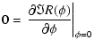
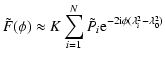
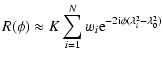
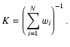
A&A 441, 1217-1228 (2005)
DOI: 10.1051/0004-6361:20052990
M. A. Brentjens1,2 - A. G. de Bruyn2,1
1 - Kapteyn Astronomical Institute, University of Groningen,
PO Box 800, 9700 AV Groningen, The Netherlands
2 -
ASTRON, PO Box 2, 7990 AA Dwingeloo, The Netherlands
Received 4 March 2005 / Accepted 20 June 2005
Abstract
We extend the rotation measure work of Burn (1966, MNRAS, 133, 67) to
the cases of limited sampling of ![]() space and non-constant
emission spectra. We introduce the rotation measure transfer function
(RMTF), which is an excellent predictor of
space and non-constant
emission spectra. We introduce the rotation measure transfer function
(RMTF), which is an excellent predictor of ![]() ambiguity problems
with the
ambiguity problems
with the ![]() coverage. Rotation measure synthesis can be
implemented very efficiently on modern computers. Because the analysis
is easily applied to wide fields, one can conduct very fast RM surveys
of weak spatially extended sources. Difficult situations, for example
multiple sources along the line of sight, are easily detected and
transparently handled. Under certain conditions, it is even possible
to recover the emission as a function of Faraday depth within a single
cloud of ionized gas. Rotation measure synthesis has already been
successful in discovering widespread, weak, polarized emission
associated with the Perseus cluster (de Bruyn & Brentjens 2005, A&A, 441, 931). In
simple, high signal to noise situations it is as good as traditional
linear fits to
coverage. Rotation measure synthesis can be
implemented very efficiently on modern computers. Because the analysis
is easily applied to wide fields, one can conduct very fast RM surveys
of weak spatially extended sources. Difficult situations, for example
multiple sources along the line of sight, are easily detected and
transparently handled. Under certain conditions, it is even possible
to recover the emission as a function of Faraday depth within a single
cloud of ionized gas. Rotation measure synthesis has already been
successful in discovering widespread, weak, polarized emission
associated with the Perseus cluster (de Bruyn & Brentjens 2005, A&A, 441, 931). In
simple, high signal to noise situations it is as good as traditional
linear fits to ![]() versus
versus ![]() plots. However, when the
situation is more complex or very weak polarized emission at high
rotation measures is expected, it is the only viable option.
plots. However, when the
situation is more complex or very weak polarized emission at high
rotation measures is expected, it is the only viable option.
Key words: methods: data analysis - techniques: polarimetric - magnetic fields - polarization - ISM: magnetic fields - Cosmology: large-scale structure of Universe
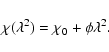
Polarization observations at radio frequencies are an important diagnostic tool in the study of galactic and extragalactic magnetic fields (e.g. Widrow 2002; Vallee 1997; Kronberg 1994). Due to birefringence of the magneto-ionic medium, the polarization angle of linearly polarized radiation that propagates through the plasma is rotated as a function of frequency. This effect is called Faraday rotation. There exist many papers describing aspects of Faraday rotation work. The most relevant ones for this work are Burn (1966), Gardner & Whiteoak (1966), Sokoloff et al. (1998), Sokoloff et al. (1999), and Vallee (1980).
![\begin{figure}
\par\includegraphics[width=8.8cm,clip]{2990fg1a.eps}\hspace*{2mm}
\includegraphics[width=8.8cm,clip]{2990fg1b.eps}\end{figure}](/articles/aa/full/2005/39/aa2990-05/img32.gif) |
Figure 1:
|
| Open with DEXTER | |
Assuming that the directions of the velocity vectors of the
electrons gyrating in a magnetized plasma are isotropically distributed,
Le Roux (1961) showed that the intrinsic degree of polarization of
synchrotron radiation from plasma in a uniform magnetic field
is given by
 |
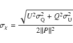
(2) |
From observations of the Crab nebula by Woltjer (1958),
Westfold (1959) determined that
![]() .
This would imply a polarization fraction of
approximately 67%, independent of frequency. In many radio sources,
the observed polarization fractions are much lower. Usually the
polarization fraction decreases steeply with increasing wavelength
(Strom & Conway 1985; Conway & Strom 1985).
.
This would imply a polarization fraction of
approximately 67%, independent of frequency. In many radio sources,
the observed polarization fractions are much lower. Usually the
polarization fraction decreases steeply with increasing wavelength
(Strom & Conway 1985; Conway & Strom 1985).
Burn (1966) discusses this depolarization effect extensively. One of the mechanisms he discusses is Faraday dispersion: emission at different Faraday depths along the same line of sight.
Following Burn (1966), we make a clear distinction between
Faraday depth (![]() )
and rotation measure (RM). We define the
Faraday depth of a source as
)
and rotation measure (RM). We define the
Faraday depth of a source as
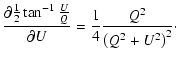
The rotation measure is commonly defined as the slope of a
polarization angle ![]() versus
versus ![]() plot:
plot:
 |
(4) |
 |
(5) |
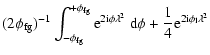
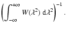
P can be written as
If there is only one source along the line of sight, which
in addition has no internal Faraday rotation, and does not suffer from
beam depolarization, then the Faraday depth of that source is equal to
its rotation measure at all wavelengths:
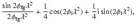
A simple example illustrates this. Imagine a classical double
radio galaxy, of which the lobe closest to us is at a Faraday depth of
![]() .
The lobe itself is
Faraday thin and has an intrinsic polarized flux density of
0.25 Jy beam-1 (positive Stokes Q). At low frequencies, there
is usually some polarized Galactic foreground emission between us and
the radio galaxy. The Galactic foreground is modelled as a uniform slab with a constant,
uniform magnetic field. The total integrated polarized surface
brightness of the Galactic foreground at
.
The lobe itself is
Faraday thin and has an intrinsic polarized flux density of
0.25 Jy beam-1 (positive Stokes Q). At low frequencies, there
is usually some polarized Galactic foreground emission between us and
the radio galaxy. The Galactic foreground is modelled as a uniform slab with a constant,
uniform magnetic field. The total integrated polarized surface
brightness of the Galactic foreground at ![]() is 1 Jy beam-1(positive Stokes Q). The Faraday dispersion function
is 1 Jy beam-1(positive Stokes Q). The Faraday dispersion function ![]() is a
top hat function:
is a
top hat function:
 |
(10) |
Figure 1 plots ![]() ,
,
![]() ,
and
,
and
![]() for Eq. (13).
for Eq. (13).
![]() is the real
part of
is the real
part of
![]() .
We have taken
.
We have taken
![]() and
and
![]() .
At low
.
At low ![]() ,
the foreground dominates over the
lobe, forcing Stokes Q of the sum of the polarizations to be
positive, while U can be both positive and negative. In this regime,
,
the foreground dominates over the
lobe, forcing Stokes Q of the sum of the polarizations to be
positive, while U can be both positive and negative. In this regime,
![]() oscillates around zero. However, when the foreground is
significantly depolarized, the lobe starts to dominate the total (Q,
U) vector. This point is reached somewhere near
oscillates around zero. However, when the foreground is
significantly depolarized, the lobe starts to dominate the total (Q,
U) vector. This point is reached somewhere near
![]() m2. From there on the total (Q, U) vector runs through
all four quadrants. As the polarized flux of the foreground vanishes,
the total polarization angle approaches more and more a straight line
corresponding to a RM of +10 rad m-2.
m2. From there on the total (Q, U) vector runs through
all four quadrants. As the polarized flux of the foreground vanishes,
the total polarization angle approaches more and more a straight line
corresponding to a RM of +10 rad m-2.
![\begin{figure}
\par\includegraphics[width=8.8cm,clip]{2990fg2.eps}\end{figure}](/articles/aa/full/2005/39/aa2990-05/img80.gif) |
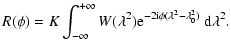
Figure 2:
Cartoon sketching the relation between emission,
|
| Open with DEXTER | |
Figure 2 shows an example of a fairly
complex line of sight. There are three areas with polarized emission
(A, B, and C), of which two (A and B) also have internal Faraday
rotation. The middle panel shows the non-monotonic relation between
Faraday depth and physical depth. Although area B is larger in
physical depth, area A is larger in Faraday depth due to the high
absolute value of
![]() .
.
A physical interpretation of this example would be that region A and its adjacent rotation-only areas reside in our Galaxy, area B and its neighboring rotation-only areas are a galaxy cluster, and area C represents a collection of distant polarized sources without any internal Faraday rotation of their own. Line of sight 1 goes through the cluster, while line of sight 2 just misses it. This causes C to be at different Faraday depth in the two lines of sight.
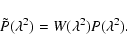
Because of the Fourier nature of both Eq. (6) and radio synthesis imaging,
there exist many analogies between the two. Examples are
uv plane sampling versus ![]() sampling and synthesized beam
versus RMTF. Therefore we prefer to call the process of inversion
"Rotation Measure synthesis'' ("RM-synthesis'' for short).
sampling and synthesized beam
versus RMTF. Therefore we prefer to call the process of inversion
"Rotation Measure synthesis'' ("RM-synthesis'' for short).
Similar methods have recently been applied to pulsar observations
(Mitra et al. 2003; Weisberg et al. 2004). de Bruyn (1996) applied
the method for the first time to an entire field of view. He also
introduced the concept of a Rotation Measure Transfer Function (RMTF,
see also Sect. 2 of this work). When
applied to a complete field of view instead of just one line of sight,
the output of a RM-synthesis is a so-called "RM-cube''. The RM-cube
has axes ![]() ,
,
![]() ,
and
,
and ![]() .
It is the Faraday rotation
equivalent of a 21 cm line cube. The application to wide fields
allowed the discovery of widespread, very faint polarized emission
associated with the Perseus cluster (de Bruyn & Brentjens 2005).
.
It is the Faraday rotation
equivalent of a 21 cm line cube. The application to wide fields
allowed the discovery of widespread, very faint polarized emission
associated with the Perseus cluster (de Bruyn & Brentjens 2005).
Modern correlator backends, like the ones installed at the WSRT, the GMRT, and the ATCA and the one to be installed at the EVLA deliver the visibilities in many (32 to 1024) narrow channels across a wide band (typically 16 to 160 MHz). The narrow channels move the bandwidth depolarization limit to much higher rotation measures. The wider bands yield very high sensitivities if the full bandwidth can be used. Thanks to these backends RM-synthesis has finally become a practical, even necessary observing method.
Section 2 discusses the generally
incomplete sampling of
![]() .
We formally derive the
RMTF. Section 3 treats
modifications to the assumption that
.
We formally derive the
RMTF. Section 3 treats
modifications to the assumption that ![]() is frequency
independent. In Sect. 4 we treat the relation between the RMTF
and
is frequency
independent. In Sect. 4 we treat the relation between the RMTF
and ![]() ambiguities in traditional RM fitting. Section 5 describes RM-synthesis with Stokes Q or
U only. Section 6 gives advice
on designing Faraday rotation experiments, taking the findings of this
work into account. Section 7 concludes
this work. Appendix A expands on error
estimation in RM work and Appendix B treats an example simulation
illustrating a few important concepts presented in this work.
ambiguities in traditional RM fitting. Section 5 describes RM-synthesis with Stokes Q or
U only. Section 6 gives advice
on designing Faraday rotation experiments, taking the findings of this
work into account. Section 7 concludes
this work. Appendix A expands on error
estimation in RM work and Appendix B treats an example simulation
illustrating a few important concepts presented in this work.
Table 1: List of symbols.
The goal of this section is to approximate
![]() by Fourier inverting a generalized version of Eq. (6).
Table 1 summarizes the symbols that
are used throughout this paper. We generalize Eq. (6) by introducing the weight
function
by Fourier inverting a generalized version of Eq. (6).
Table 1 summarizes the symbols that
are used throughout this paper. We generalize Eq. (6) by introducing the weight
function
![]() .
.
![]() is also called the sampling
function. It is nonzero at all
is also called the sampling
function. It is nonzero at all ![]() points where measurements
are taken. It is zero elsewhere. Obviously,
points where measurements
are taken. It is zero elsewhere. Obviously,
![]() for
for
![]() because of the lack of measurements there. The
observed polarized flux density, or surface brightness in the case of
spatially extended sources, is
because of the lack of measurements there. The
observed polarized flux density, or surface brightness in the case of
spatially extended sources, is
 |
(19) |
![\begin{figure}
\par\includegraphics[width=8.5cm,clip]{2990fg3.eps}\end{figure}](/articles/aa/full/2005/39/aa2990-05/img136.gif) |
Figure 3:
RMTF of a 92 cm dataset taken with the Westerbork Synthesis
Radio Telescope. There are 126 usable channels in the dataset. All
(Q,U) vectors have been derotated to
|
| Open with DEXTER | |
The above set of equations is not yet our final result.
Figure 3 displays the rotation measure transfer
function corresponding to the ![]() sampling of our Perseus data
set (de Bruyn & Brentjens 2005). It only shows a small part of the
RMTF close to the peak. The response function displays a rapid
rotation of the (real, imaginary) vector. Because one usually samples
sampling of our Perseus data
set (de Bruyn & Brentjens 2005). It only shows a small part of the
RMTF close to the peak. The response function displays a rapid
rotation of the (real, imaginary) vector. Because one usually samples
![]() space at finite intervals, this rotation makes it very
difficult to correctly estimate the polarization angle at or near the
maximum of
space at finite intervals, this rotation makes it very
difficult to correctly estimate the polarization angle at or near the
maximum of
![]() .
If the Faraday depth of a frame is only a tenth
of the width of the RMTF away from the actual Faraday depth of the
source, the (real, imaginary) vector may already be rotated by
several tens of degrees.
.
If the Faraday depth of a frame is only a tenth
of the width of the RMTF away from the actual Faraday depth of the
source, the (real, imaginary) vector may already be rotated by
several tens of degrees.
Equations (22) and (23) correspond to derotating all polarization
vectors back to their position at
![]() .
At first this appears
sensible, because the polarization vector at
.
At first this appears
sensible, because the polarization vector at
![]() is directly
related to the electric field vector in the plane of the
sky without any Faraday rotation. Nevertheless no information is lost by
derotating to some other common
is directly
related to the electric field vector in the plane of the
sky without any Faraday rotation. Nevertheless no information is lost by
derotating to some other common
![]() .
.
The more general versions of Eqs. (22) and (23) are
The simplest way to see this is to consider the case when
![]() .
This changes the
convolution in Eq. (25) into a
multiplication. Hence the result of the righthand side of Eq. (25) can be written as
.
This changes the
convolution in Eq. (25) into a
multiplication. Hence the result of the righthand side of Eq. (25) can be written as
 |
(27) |
Ideally, the response in the entire main peak of the RMTF
should be parallel to the actual polarization vector at
![]() .
The best way of achieving that is keeping the orthogonal
response as close to zero as possible. We set the derivative of the
imaginary part at
.
The best way of achieving that is keeping the orthogonal
response as close to zero as possible. We set the derivative of the
imaginary part at ![]() to zero:
to zero:
A drawback of having
![]() is that the polarization
angle that one derives still needs to be transformed to a polarization
angle at
is that the polarization
angle that one derives still needs to be transformed to a polarization
angle at
![]() ,
if one wants information on the orientation
of the electric field direction in the source. In case of a
high S/N ratio, this is very easy:
,
if one wants information on the orientation
of the electric field direction in the source. In case of a
high S/N ratio, this is very easy:
 |
(33) |
![\begin{figure}
\par\includegraphics[width=8.5cm,clip]{2990fg4.eps}\end{figure}](/articles/aa/full/2005/39/aa2990-05/img160.gif) |
Figure 4:
RMTF of the same dataset as described in
Fig. 3. This time, however, all |
| Open with DEXTER | |
Figure 4 shows the same RMTF as
Fig. 3, except that
![]() is set to
the weighted average
is set to
the weighted average ![]() .
The improvement with respect to the
orthogonal response is evident. The response function is almost
completely real between the first minima. The only drawback is that
one cannot convert the observed polarization angle at
.
The improvement with respect to the
orthogonal response is evident. The response function is almost
completely real between the first minima. The only drawback is that
one cannot convert the observed polarization angle at ![]() to a
to a
![]() vector in a straightforward way. In order to accomplish
reliable derotation to
vector in a straightforward way. In order to accomplish
reliable derotation to
![]() ,
one needs a sufficiently high
S/N ratio to determine the Faraday depth with an accuracy well within
the full width at half maximum (FWHM) of the RMTF. This is
not a problem for bright sources that are already detected in
individual channels, but for faint emission that is only detectable
after RM-synthesis, one cannot usually do this. These signal to noise
statements are quantified in Sect. 4
and Appendix A.
,
one needs a sufficiently high
S/N ratio to determine the Faraday depth with an accuracy well within
the full width at half maximum (FWHM) of the RMTF. This is
not a problem for bright sources that are already detected in
individual channels, but for faint emission that is only detectable
after RM-synthesis, one cannot usually do this. These signal to noise
statements are quantified in Sect. 4
and Appendix A.
In most correlators, all channels have equal bandwidth ![]() ,
centred
around
,
centred
around
![]() ,
the central frequency of the channel. Our
prime coordinate is
,
the central frequency of the channel. Our
prime coordinate is ![]() ,
not
,
not ![]() .
If we assume a top hat
channel bandpass, we have for every channel:
.
If we assume a top hat
channel bandpass, we have for every channel:
If
![]() for all channels, we may approximate
the integrals in Eqs. (25) and (26) by sums:
for all channels, we may approximate
the integrals in Eqs. (25) and (26) by sums:
In this section we investigate the effect of the emission spectrum of
a source on the method. We start with the most general case of an
arbitrary spectrum at each Faraday depth. We substitute
 |
(39) |
 |
(40) |
The second case is a specialization of the first case. Equation (44) reduces to Eq. (15) in case of a flat
spectrum. The approximate Faraday dispersion function compensated for
a non-flat spectrum is given by:
 |
(45) |
Equation (42) applies only in some very
specific scenarios. It holds for example in optically thin
synchrotron-emitting and Faraday-rotating clouds that have the same
relativistic electron energy distribution throughout the
cloud. It also holds if multiple optically thin clouds along the line
of sight happen to have the same spectral dependence. Optically thin
synchrotron radiation has a spectrum that is proportional to
![]() over a large range of frequencies
(Conway et al. 1963). For most sources,
over a large range of frequencies
(Conway et al. 1963). For most sources,
![]() is in the range
is in the range
![]() .
In extreme cases
the spectral index of optically thin emission can approach 0
(e.g. the Crab nebula) or -3 (for halo or relic sources in galaxy
clusters).
.
In extreme cases
the spectral index of optically thin emission can approach 0
(e.g. the Crab nebula) or -3 (for halo or relic sources in galaxy
clusters).
In general, spectral indices vary across a map. One can of course easily correct for the spectra of sources that are reliably detected in individual channel maps. This is impossible for sources that are much fainter and only show up after averaging the full band. For those objects it makes sense to estimate some "average'' spectral index and apply that to the entire map.
What is the effect of using the wrong spectral index in correcting for the spectrum of a single source along the line of sight? The contributions of multiple sources along the line of sight is simply the sum of their individual responses. Because the spectrum is an amplitude only effect, it has no influence on the location of the maximum of the Faraday dispersion function of the source. Therefore its derived Faraday depth is unaffected. It does distort the RMTF associated with the source at points away from the main peak. This complicates deconvolution algorithms slightly.
![\begin{figure}
\par\includegraphics[width=8.5cm,clip]{2990fg5.eps}\end{figure}](/articles/aa/full/2005/39/aa2990-05/img189.gif) |
Figure 5:
Absolute value of the approximated Faraday dispersion
function of several Faraday thin sources with different spectral
indices. The |
| Open with DEXTER | |
Figure 5 gives the Faraday
dispersion functions of Faraday thin model sources with spectral
indices -3 to 0. It is seen that the largest effect
occurs close to the nulls of the RMTF. The difference
between
![]() and
and
![]() is small over the 17% total
frequency bandwidth in the simulation. It will not be noticeable if
the emission has such low S/N that it is invisible in individual
channels. For comparison, the normalized
is small over the 17% total
frequency bandwidth in the simulation. It will not be noticeable if
the emission has such low S/N that it is invisible in individual
channels. For comparison, the normalized
![]() of a
Faraday thick uniform slab model is included. The slab emits at
of a
Faraday thick uniform slab model is included. The slab emits at
![]() .
It is seen that the
effect of even a tiny amount of
.
It is seen that the
effect of even a tiny amount of ![]() structure in the source is
much larger than the effect of changing the spectral index by
structure in the source is
much larger than the effect of changing the spectral index by ![]() .
.
The general case of an arbitrary spectral dependence at multiple Faraday depths is not invertible. One can only recover the Faraday dispersion function if the spectral dependence is the same at all Faraday depths along the line of sight. One should then divide the observed polarization by the spectral dependence in I. Figure 5 shows that if the spectral index is estimated with an absolute uncertainty less than 1, the maximum absolute error of the estimated flux density at a certain Faraday depth is less than 2-5% of the brightest emission along the line of sight. This accuracy is easily exceeded for sources that are visible in total intensity. Sources that have not been detected in total intensity should generally be assigned a spectral index of -1. This worked very well in our observations of the Perseus cluster, where we see large, faint polarized features that have no detectable counterpart in total intensity (de Bruyn & Brentjens 2005).
The traditional way to compute the rotation measure of a source is to
measure its polarization angle at several wavelengths and determine
the slope of a straight line through the polarization angle as a
function of ![]() .
This method suffers from so-called
.
This method suffers from so-called ![]() ambiguity problems. If only a few data points are available, there may
exist multiple RM solutions that are equally good, but have the
polarization angle of the data points wrapped around one or more
turns. Complicated methods have been devised to attempt to circumvent
these problems, some of which are quite successful. An example is the
"Pacerman'' method (Vogt et al. 2004; Dolag et al. 2004), which operates on images,
and does a good job in finding and correcting
ambiguity problems. If only a few data points are available, there may
exist multiple RM solutions that are equally good, but have the
polarization angle of the data points wrapped around one or more
turns. Complicated methods have been devised to attempt to circumvent
these problems, some of which are quite successful. An example is the
"Pacerman'' method (Vogt et al. 2004; Dolag et al. 2004), which operates on images,
and does a good job in finding and correcting ![]() ambiguities using
spatial continuity arguments.
ambiguities using
spatial continuity arguments.
In this section we show that the RMTF is an excellent indicator of
possible ![]() ambiguity problems. By analyzing the RMTF, one can
take measures to minimize or even eradicate any potential
ambiguity problems. By analyzing the RMTF, one can
take measures to minimize or even eradicate any potential ![]() problems in the experiment in advance. We also show that using
only RM-synthesis to determine Faraday depths is as
accurate as traditional
problems in the experiment in advance. We also show that using
only RM-synthesis to determine Faraday depths is as
accurate as traditional ![]() fitting, but has the added value
of straightforward
fitting, but has the added value
of straightforward ![]() ambiguity problem detection.
ambiguity problem detection.
We first consider traditional ![]() fitting. This is done by
linear least squares minimization of a merit function
fitting. This is done by
linear least squares minimization of a merit function ![]() .
If the
estimated errors of all points are equal, then the merit function
looks like Eq. (49)
.
If the
estimated errors of all points are equal, then the merit function
looks like Eq. (49)
![\begin{figure}
\par\includegraphics[width=8.3cm,clip]{2990fg6.eps}\end{figure}](/articles/aa/full/2005/39/aa2990-05/img208.gif) |
Figure 6:
Comparison of merit function |
| Open with DEXTER | |
![\begin{figure}
\par\mbox{
\includegraphics[width=8.7cm,clip]{2990fg7a.eps}\hspace*{2mm}
\includegraphics[width=8.7cm,clip]{2990fg7b.eps} }
\end{figure}](/articles/aa/full/2005/39/aa2990-05/img210.gif) |
Figure 7:
Both plots show, from top to bottom, merit function |
| Open with DEXTER | |
![\begin{figure}
\mbox{
\includegraphics[width=8.7cm,clip]{2990fg8a.eps}\hspace*{2mm}
\includegraphics[width=8.7cm,clip]{2990fg8b.eps} }
\end{figure}](/articles/aa/full/2005/39/aa2990-05/img211.gif) |
Figure 8: This plot shows the effect of tweaking the exact frequencies of eight sampling points. The lefthand panel shows the same RMTF as the lefthand panel of Fig. 7. In the righthand plot, however, we stretched the frequency intervals such that low frequency intervals are wider than high frequency intervals. This eliminates the resonances from the lefthand plot. |
| Open with DEXTER | |
If the model RM is sufficiently different from the actual RM, one
expects the errors li to be approximately uniformly distributed in
the range
![]() .
Because the square is taken, this is
equivalent to a uniform distribution in the range
.
Because the square is taken, this is
equivalent to a uniform distribution in the range
![]() .
The average value of li2 is then
given by
.
The average value of li2 is then
given by
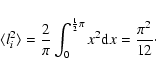 |
(51) |
An interesting aspect seen in
Fig. 6 is that the envelope of
![]() looks like
looks like ![]() when
when
![]() .
Deep
minima of
.
Deep
minima of ![]() are associated with high peaks in the
RMTF. In fact, they appear to be approximately proportional to
are associated with high peaks in the
RMTF. In fact, they appear to be approximately proportional to
![]() .
These deep minima are closely related to so-called
.
These deep minima are closely related to so-called
![]() ambiguities in traditional RM measurements. They
are points that fit the data (almost) equally well as the "true''
solution.
ambiguities in traditional RM measurements. They
are points that fit the data (almost) equally well as the "true''
solution.
The similarity between the envelope of ![]() and
and ![]() is better demonstrated in Fig. 7.
It shows both
is better demonstrated in Fig. 7.
It shows both ![]() and
and ![]() over a large range in
over a large range in
![]() .
The lefthand panel displays
.
The lefthand panel displays ![]() and
and ![]() for 8 points,
equally spaced in frequency. To facilitate comparison, the total
width of the pattern,
for 8 points,
equally spaced in frequency. To facilitate comparison, the total
width of the pattern,
![]() ,
has been scaled to match the
width of the
,
has been scaled to match the
width of the ![]() sampling of
Fig. 6. The righthand panel of
Fig. 7 shows
sampling of
Fig. 6. The righthand panel of
Fig. 7 shows ![]() and
and ![]() based
on the same input data as Fig. 6.
It is obvious that the RMTF of a 126 point sampling has much lower
side lobes than an 8-point sampling.
based
on the same input data as Fig. 6.
It is obvious that the RMTF of a 126 point sampling has much lower
side lobes than an 8-point sampling. ![]() ambiguities are
completely eliminated.
ambiguities are
completely eliminated.
The lefthand panel of Fig. 8 shows the
same RMTF as the lefthand panel of
Fig. 7. The two resonances to the left
and right are due to the near-regularity of the sampling
points in ![]() space. If the frequency intervals at the lower
frequencies are stretched more than at the intervals at
higher frequencies, for example by making them decrease linearly with
increasing frequency, one can make the pattern in
space. If the frequency intervals at the lower
frequencies are stretched more than at the intervals at
higher frequencies, for example by making them decrease linearly with
increasing frequency, one can make the pattern in ![]() space
less regular. The result is shown in the righthand panel of
Fig. 8. The resonances are now lower and
wider. If one requires the highest side lobes to be at least 5
space
less regular. The result is shown in the righthand panel of
Fig. 8. The resonances are now lower and
wider. If one requires the highest side lobes to be at least 5![]() lower than unity, then a total S/N of 20 (7 per channel) is sufficient
to prevent
lower than unity, then a total S/N of 20 (7 per channel) is sufficient
to prevent ![]() ambiguities outside the main peak of the RMTF. Using
the same requirement, in case of the 126 points, a S/N of 6 in total
(0.6 per channel) is enough to prevent
ambiguities outside the main peak of the RMTF. Using
the same requirement, in case of the 126 points, a S/N of 6 in total
(0.6 per channel) is enough to prevent ![]() ambiguities outside the
main peak of the RMTF.
ambiguities outside the
main peak of the RMTF.
![]() ambiguities are conceptually closely related to the grating
response of a regularly spaced interferometer like the WSRT. When an
interferometer only has baselines that are a multiple of some fixed
distance, then its instantaneous synthesized beam is a collection of
parallel fan beams. Each fan beam has the same peak amplitude.
Therefore, without any further constraints it is impossible to
determine in which fan beam the source is actually located. The same
holds true for
ambiguities are conceptually closely related to the grating
response of a regularly spaced interferometer like the WSRT. When an
interferometer only has baselines that are a multiple of some fixed
distance, then its instantaneous synthesized beam is a collection of
parallel fan beams. Each fan beam has the same peak amplitude.
Therefore, without any further constraints it is impossible to
determine in which fan beam the source is actually located. The same
holds true for ![]() sampling. If one only samples
sampling. If one only samples ![]() space at regular intervals, there exist multiple solutions that fit
the data equally well. These solutions correspond to peaks of unit
amplitude in the RMTF: grating responses.
space at regular intervals, there exist multiple solutions that fit
the data equally well. These solutions correspond to peaks of unit
amplitude in the RMTF: grating responses.
Figure 6 also shows that there
are multiple minima of ![]() within the main lobe of the RMTF. These
indicate uncertainties in the RM smaller than the width of the main
peak. We shall now investigate the uncertainty in RM within the main
peak of
within the main lobe of the RMTF. These
indicate uncertainties in the RM smaller than the width of the main
peak. We shall now investigate the uncertainty in RM within the main
peak of ![]() .
.
The standard error in the RM when obtained by fitting a straight line
to a plot of ![]() versus
versus ![]() is given by
is given by
 |
(54) |
 |
(55) |
In RM-synthesis, one determines the RM of a single source along the
line of sight by fitting, for example, a parabola to the main peak of
![]() .
The detailed procedure is to first find the brightest
point in a critically sampled Faraday dispersion function (2-3 points
per
.
The detailed procedure is to first find the brightest
point in a critically sampled Faraday dispersion function (2-3 points
per
![]() ), covering a wide range in
), covering a wide range in ![]() .
This is followed
by oversampling the region around the peak by a large factor. A
parabolic fit to the 10-20 points directly surrounding the peak then
yields the RM of the source.
.
This is followed
by oversampling the region around the peak by a large factor. A
parabolic fit to the 10-20 points directly surrounding the peak then
yields the RM of the source.
We have simulated this procedure in order to get a quantitative idea
of the typical error in RM that one obtains, given a certain noise
level in the Stokes Q and U images, and a certain set of sample
points
![]() .
The results are shown in
Fig. 9. The total signal-to-noise ratio is
equal to
.
The results are shown in
Fig. 9. The total signal-to-noise ratio is
equal to
![]() .
The solid line is Eq. (52). The points are standard deviations in
RM computed from 1000 iterations per S/N ratio point. We have assumed
the noise in Stokes Q and U to be equal and Gaussian. We see
excellent agreement with the error expected for traditional
.
The solid line is Eq. (52). The points are standard deviations in
RM computed from 1000 iterations per S/N ratio point. We have assumed
the noise in Stokes Q and U to be equal and Gaussian. We see
excellent agreement with the error expected for traditional
![]() fitting (the straight line). At a S/N ratio less than 4,
the points deviate strongly from the line. This is due to the fact
that the non-Gaussianity of the noise in P is only noticeable close
to the origin of the complex plane. It is stressed that a total S/N of
4 when having 126 channels implies a S/N per channel of slightly less
than 0.4. It is impossible to determine a polarization
angle with such a low S/N in the case of standard
fitting (the straight line). At a S/N ratio less than 4,
the points deviate strongly from the line. This is due to the fact
that the non-Gaussianity of the noise in P is only noticeable close
to the origin of the complex plane. It is stressed that a total S/N of
4 when having 126 channels implies a S/N per channel of slightly less
than 0.4. It is impossible to determine a polarization
angle with such a low S/N in the case of standard ![]() fitting.
fitting.
It is also possible to perform a RM-synthesis with Stokes Q or Uonly. There exist many radio observations that have produced only Stokes I and Q, for example spectral line work with arrays equipped with linearly polarized feeds, or data from backends with limited correlator capacity. However, by using only one of the two Stokes parameters, one loses information about the sign of the Faraday depth.
![\begin{figure}
\par\includegraphics[width=8.6cm]{2990fg9.eps}\end{figure}](/articles/aa/full/2005/39/aa2990-05/img233.gif) |
Figure 9:
Comparison between the standard error in RM obtained by
traditional line fitting (line) to simulated RM-synthesis experiments
where a parabola was fit to the main peak of the Faraday dispersion
function (dots). The 126 |
| Open with DEXTER | |
The derivation is started with Eq. (25). The identities
 |
(59) | ||
 |
(60) |
![\begin{figure}
\par\includegraphics[width=16cm,clip]{2990fg10.eps}\end{figure}](/articles/aa/full/2005/39/aa2990-05/img241.gif) |
Figure 10:
Comparison of Q-only RM-synthesis ( left) and Q+URM-synthesis ( right) for Faraday depths
|
| Open with DEXTER | |
Figure 10 compares
results of a complete RM-synthesis of data of the Perseus cluster,
taken with the WSRT (de Bruyn & Brentjens 2005), to results of a
Q-only RM-synthesis of the same dataset. It compares both the
Galactic foreground emission at low Faraday depth, and the emission at
higher Faraday depth that we attribute to the Perseus cluster. It is
clearly seen that the noise in the Q-only images is increased with
respect to the complete RM-synthesis. The bar-like feature at
![]() ,
,
![]() is already visible in the Q-only images. This
demonstrates that one actually can detect faint emission at high
Faraday depths using only Stokes Q or U images. Unless the
situation is simple, meaning only one discrete source along the line
of sight, these images are unfortunately not useful in a quantitative
sense. However, it is an efficient way to discover weak, Faraday
rotated, polarized emission in existing datasets, which can
then be followed up with full polarization observations.
is already visible in the Q-only images. This
demonstrates that one actually can detect faint emission at high
Faraday depths using only Stokes Q or U images. Unless the
situation is simple, meaning only one discrete source along the line
of sight, these images are unfortunately not useful in a quantitative
sense. However, it is an efficient way to discover weak, Faraday
rotated, polarized emission in existing datasets, which can
then be followed up with full polarization observations.
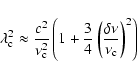
Three main parameters are involved when planning a rotation-measure
experiment, namely the channel width
![]() ,
the width of
the
,
the width of
the ![]() distribution
distribution
![]() ,
and the shortest
wavelength squared
,
and the shortest
wavelength squared
![]() .
They are summarized in
Fig. 11. These parameters determine
respectively the maximum observable Faraday depth, the resolution in
.
They are summarized in
Fig. 11. These parameters determine
respectively the maximum observable Faraday depth, the resolution in
![]() space, and the largest scale in
space, and the largest scale in ![]() space to which one is
sensitive. Estimates for the FWHM of the main peak of the RMTF, the
scale in
space to which one is
sensitive. Estimates for the FWHM of the main peak of the RMTF, the
scale in ![]() space to which sensitivity has dropped to 50% and
the maximum Faraday depth to which one has more than 50% sensitivity
are approximately
space to which sensitivity has dropped to 50% and
the maximum Faraday depth to which one has more than 50% sensitivity
are approximately
It is interesting to compare Eqs. (61) and (62). This is where the analogy between RM-synthesis and regular synthesis imaging breaks down. In synthesis imaging, the width of the synthesized beam is inversely proportional to the maximum absolute uv vector. That is, the distance between the origin and the uvpoint most distant from it. The maximum scale that one can measure depends on the shortest baseline. Therefore one is always maximally sensitive to structures smaller than the width of the synthesized beam.
| |
Figure 11: The three instrumental parameters that determine the output of a Faraday rotation experiment. |
| Open with DEXTER | |
This is quite different in RM-synthesis. In RM-synthesis it
is possible that a source is unresolved in the sense that its extent
in ![]() is less than the width of the RMTF, yet "resolved'' out
because one has not sampled the typical
is less than the width of the RMTF, yet "resolved'' out
because one has not sampled the typical ![]() -scale of the source due
to lack of small
-scale of the source due
to lack of small ![]() points. Equation (61) shows that the width of the RMTF
depends on the width of the
points. Equation (61) shows that the width of the RMTF
depends on the width of the ![]() distribution, not on the
largest
distribution, not on the
largest ![]() measured. Nevertheless the largest scale in
measured. Nevertheless the largest scale in ![]() that one is sensitive to is set by the smallest
that one is sensitive to is set by the smallest ![]() as is
shown in Eq. (62). In order to truly
resolve Faraday thick clouds in
as is
shown in Eq. (62). In order to truly
resolve Faraday thick clouds in ![]() space in the sense that one
could see internal structure, the main peak of the RMTF should be
narrower than the maximum scale to which one is sensitive. Because
space in the sense that one
could see internal structure, the main peak of the RMTF should be
narrower than the maximum scale to which one is sensitive. Because
![]() ,
the requirement for resolving Faraday thick
structures is
,
the requirement for resolving Faraday thick
structures is
For deconvolution the RMTF should be known as accurately as possible for all sources within the field of view and along the line of sight. The main problems are:
After primary beam correction, one should align the channel maps
spectrally. Our preferred method is to determine the average
total intensity of a large sample of sources, and scale the images until
the average of the ensemble in a particular channel map matches the
value at
![]() .
Using this approach, the
spectra of as yet undetected emission should be approximately flat to
within a spectral index range of
.
Using this approach, the
spectra of as yet undetected emission should be approximately flat to
within a spectral index range of ![]() .
Of course one could flatten
source spectra on an individual basis. This is only useful if one is
interested in bright sources that are easily detected in individual
channels.
.
Of course one could flatten
source spectra on an individual basis. This is only useful if one is
interested in bright sources that are easily detected in individual
channels.
A convenient property of RM-synthesis is that more-or-less frequency
independent instrumental problems end up at ![]() ,
convolved with the RMTF. This means that instrumental problems are
highly reduced at higher absolute Faraday depths. In other words: at
high Faraday depth, we "wind-up'' the instrumental polarization
problems, while "unwinding'' the Faraday rotated cosmic polarization
signals.
,
convolved with the RMTF. This means that instrumental problems are
highly reduced at higher absolute Faraday depths. In other words: at
high Faraday depth, we "wind-up'' the instrumental polarization
problems, while "unwinding'' the Faraday rotated cosmic polarization
signals.
We have extended the work of Burn (1966) to the cases of limited
sampling of ![]() space and some spectral dependencies. We have
introduced the RMTF, which is an excellent predictor of
space and some spectral dependencies. We have
introduced the RMTF, which is an excellent predictor of ![]() ambiguity problems in the frequency setup. RM-synthesis can be
implemented very efficiently on modern computers. For example, a RM-
synthesis of 126 input maps of 10242 pixels, yielding
ambiguity problems in the frequency setup. RM-synthesis can be
implemented very efficiently on modern computers. For example, a RM-
synthesis of 126 input maps of 10242 pixels, yielding
![]() output maps of 10242 pixels (P, Q, and U) takes less than 5 min on a laptop equipped with a 2 GHz Intel Pentium processor and
512 MB of RAM.
output maps of 10242 pixels (P, Q, and U) takes less than 5 min on a laptop equipped with a 2 GHz Intel Pentium processor and
512 MB of RAM.
Because the analysis is easily applied to wide fields, one can conduct very fast RM surveys of weak sources. Difficult situations, for example multiple sources along the line of sight, are easily detected. Under certain conditions, it is even possible to recover the emission as a function of Faraday depth within a single cloud of ionized gas.
Instrumental problems that are weakly frequency independent, or have a very characteristic frequency dependence, are easily separated from cosmic signals that are only subject to Faraday rotation.
Rotation measure synthesis has already been successful in discovering
widespread, weak, polarized emission associated with the Perseus cluster
(de Bruyn & Brentjens 2005). In simple, high signal to noise
situations it is as good as traditional linear fits to ![]() versus
versus
![]() plots. However, when the situation is more complex, or
very weak polarized emission at high rotation measures is expected, it
is the only viable option.
plots. However, when the situation is more complex, or
very weak polarized emission at high rotation measures is expected, it
is the only viable option.
Acknowledgements
We acknowledge Robert Braun, Torsten Enßlin and Peter Katgert for useful and vivid discussions on the subject. The Westerbork Synthesis Radio Telescope is operated by ASTRON (Netherlands Foundation for Research in Astronomy) with support from the Netherlands Foundation for Scientific Research (NWO).
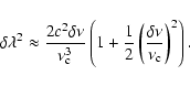
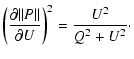
The expected standard errors in RM/Faraday depth and ![]() are
useful quantities when planning a rotation measure experiment. In this
appendix we present a formal derivation.
are
useful quantities when planning a rotation measure experiment. In this
appendix we present a formal derivation.
| (A.1) | |||
| (A.2) |
The derivation is done in two steps. First we derive the standard
error in the polarization angle and total polarization,
![]() and
and
![]() of measurements in individual
channels. Then we apply standard results for the least squares fit of
a straight line to obtain
of measurements in individual
channels. Then we apply standard results for the least squares fit of
a straight line to obtain
![]() and
and
![]() ,
the
standard errors in rotation measure / Faraday depth and the
polarization angle at
,
the
standard errors in rotation measure / Faraday depth and the
polarization angle at
![]() .
.
Error propagation (Squires 2001) gives us
 |
(A.9) | ||
 |
(A.10) |
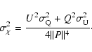 |
(A.11) |
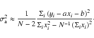 |
(A.13) |
Equation (A.16) may now be simplified by substituting Eqs. (A.17) and (A.12). The final result is:
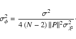 |
(A.18) |
 |
(A.19) |
 |
(A.20) |
In this appendix we show, as an illustration, three model runs of an RM-synthesis of an artificial Faraday dispersion function, measured with a realistic frequency sampling. We hope that these figures aid in understanding the most important aspects of RM-synthesis specifically and rotation measure work in general.
Sources that are extended in the plane of the sky have their surface
brightness measured in Jy per steradian. For point sources the flux in Jy
is sufficient to characterize it. The respective brightness units for
sources that are both extended in the plane of the sky and in Faraday
depth are Jy steradian-1 (rad m-2)-1 or Jy m2rad-3. Sources that are extended in the plane of the sky and
point-like in ![]() space have their brightness in
space have their brightness in ![]() space
measured in Jy steradian-1. The brightness of the measured
Faraday dispersion function has units of Jy (beam on the sky)-1(rmtf)-1. Sources that are point-like in the plane of the sky
have the steradian-1 or (beam on the sky)-1 removed.
space
measured in Jy steradian-1. The brightness of the measured
Faraday dispersion function has units of Jy (beam on the sky)-1(rmtf)-1. Sources that are point-like in the plane of the sky
have the steradian-1 or (beam on the sky)-1 removed.
In order to keep the units simple, we made all simulated sources point-like in the sky plane. Hence the units used in the figures in this appendix are:
The RMTF in all three figures is the same because the pattern and
width of the ![]() coverage is exactly the same for all of
them. The only difference is the absolute position of the
pattern. Figure B.1 has
coverage is exactly the same for all of
them. The only difference is the absolute position of the
pattern. Figure B.1 has
![]() ,
Fig. B.2 has
,
Fig. B.2 has
![]() ,
and Fig. B.3 has
,
and Fig. B.3 has
![]() .
.
The three sources in this simulation have different properties to illustrate different cases.
Source B represents the other extreme. Being several RMTFs wide, one
requires
![]() in order to
recover the full flux of the source. Only
Fig. B.1 meets this requirement. In
Fig. B.2, only two bumps at the edges
of the source remain. Because in
Fig. B.2 we only sample smaller scales
in
in order to
recover the full flux of the source. Only
Fig. B.1 meets this requirement. In
Fig. B.2, only two bumps at the edges
of the source remain. Because in
Fig. B.2 we only sample smaller scales
in ![]() due to the larger
due to the larger
![]() ,
the only parts
of source B that remain are the parts where these smaller scales are
important: the edges. Source B has practically disappeared in
Fig. B.3.
,
the only parts
of source B that remain are the parts where these smaller scales are
important: the edges. Source B has practically disappeared in
Fig. B.3.
Source C is of an intermediate type. Because its typical ![]() -scale is
narrower than source B, there is a larger fraction of the total flux
recovered in Figs. B.2 and B.3.
-scale is
narrower than source B, there is a larger fraction of the total flux
recovered in Figs. B.2 and B.3.
In analogy to radio interferometric observations, one could state that
the ![]() sampling in
Fig. B.1 corresponds to a connected
element array, where one samples all scales up to
sampling in
Fig. B.1 corresponds to a connected
element array, where one samples all scales up to
![]() approximately equally well.
Figure B.3 corresponds to a VLBI
observation, where one misses the short spacings and therefore is
insensitive to extended emission. A fundamental difference with radio
interferometry is that the resolution in
approximately equally well.
Figure B.3 corresponds to a VLBI
observation, where one misses the short spacings and therefore is
insensitive to extended emission. A fundamental difference with radio
interferometry is that the resolution in ![]() space is determined by
the width of the
space is determined by
the width of the ![]() distribution,
distribution,
![]() ,
and not
by the largest
,
and not
by the largest ![]() sampled. Hence one could encounter
situations where a source is not resolved in the sense that the
thickness of the source in
sampled. Hence one could encounter
situations where a source is not resolved in the sense that the
thickness of the source in ![]() is much less than the width of the
RMTF, while at the same time it is resolved out in the sense
that one has not sampled sufficiently short
is much less than the width of the
RMTF, while at the same time it is resolved out in the sense
that one has not sampled sufficiently short ![]() points to
detect the source.
points to
detect the source.


![$\displaystyle \left\{\begin{array}{lcr}
z_i & &z_i < \frac{1}{2}\pi\\ [2mm]
z_i-\pi & &z_i \ge \frac{1}{2}\pi
\end{array}\right.$](/articles/aa/full/2005/39/aa2990-05/img195.gif)

![\begin{displaymath}\rho = N^{-1} \sum_{i=1}^{N} \left(\left[\mbox{RM}\lambda_i^2\right]
\ \mbox{mod}\ \frac{\pi}{2}\right)^2.
\end{displaymath}](/articles/aa/full/2005/39/aa2990-05/img201.gif)


![\begin{figure}
\par\includegraphics[width=17.2cm,clip]{2990fgB1.eps}\end{figure}](/articles/aa/full/2005/39/aa2990-05/img287.gif)
![\begin{figure}
\par\includegraphics[width=17.2cm,clip]{2990fgB2.eps}\end{figure}](/articles/aa/full/2005/39/aa2990-05/img289.gif)
![\begin{figure}
\par\includegraphics[width=17.2cm,clip]{2990fgB3.eps}\end{figure}](/articles/aa/full/2005/39/aa2990-05/img291.gif)