A&A 441, 783-790 (2005)
DOI: 10.1051/0004-6361:20053327
Research Note
P. A. Dybczynski
Astronomical Observatory of the A. Mickiewicz University, S![]() oneczna 36,
60-286 Poznan, Poland
oneczna 36,
60-286 Poznan, Poland
Received 28 April 2005 / Accepted 22 June 2005
Abstract
This is the second in a series of papers presenting an attempt to
reproduce the mechanisms acting currently on the Oort cloud of comets
(Oort 1950, Bull. Astron. Inst. Nether., 11, 91) and producing the observed sample of long-period
comets. We combine the effect of the close, recent stellar passage
with the continuous action of the Galactic tidal perturbation, and
concentrate on the dominant term of this effect, namely the tidal
force induced by the galactic disk matter. The main results presented
in the previous paper of this series are fully confirmed within a
much more realistic model. The results we obtained is that the observable
subpopulation of the Oort cometary cloud remained the same in number,
even after the close stellar passage. The main output of such a passage
is a short time variation in the observable influx of comets and strong
asymmetries present in their perihelion direction distribution.
Key words: comets: general - Oort cloud - solar system: general
In the first paper of this series (Dybczynski 2002c, hereafter Paper I) we presented a detailed analysis of the separate stellar effect on the cometary cloud. We introduced two different numerical models of the cloud itself and calculated probabilities of various cometary end-states as a function of stellar passage geometrical and dynamical parameters. In addition, we discussed the asymmetries in the sample of the observable comets resulting from the stellar impulse on the cloud. The reader can find additional details of some peculiar cases in (Dybczynski 2002b,a). In the present paper we concentrate on the simultaneous action of the single stellar passage and of the Galactic disk tide. The main purpose of this paper is to demonstrate the results of a single stellar passage through or near the Oort cometary cloud under the simultaneous influence of galactic perturbations. In Sects. 2 and 3 we briefly present the nature and output of galactic perturbations, in Sect. 4 we discuss the way of superposition of stellar and Galactic perturbations, in Sect. 5 we describe "dynamical filtering'', an useful tool for speeding the calculations up, in Sect. 6 we present a detailed scheme of our Monte Carlo simulation code and finally in Sects. 7 and 8 we describe results of our simulations.
Among the first papers on the Galactic perturbations on Oort cloud
comets one should mention those by Byl (1986,1983), Harrington (1985),
Heisler & Tremaine (1986) and Matese & Whitman (1989). After recognizing
that the tidal action of the galactic disk matter is about ten times
stronger than the influence of the Galactic center, the simple dynamical
model was proposed to omit the latter, giving the following set of
equations of motion:
In some recent papers on galactic perturbations on the Oort cloud comets (Matese & Lissauer 2002; Brasser 2001; Levison et al. 2001), the authors use the extended models for the Galactic perturbations, accounting for the perturbations from the Galactic center. However, the simple model presented above is quite sufficient for our purpose. Inclusion of the influence of the Galactic center is not necessary here because we follow the cometary motion on relatively short time intervals of only several million years. Pretka (1998) has already shown that different models of the Galactic potential give significant differences only after a substantially longer time. For this reason the objections of Matese & Whitmire (1996) do not apply in our case.
The effects of the galactic disk tidal force on cometary motion described by Eqs. (1) were studied in detail in many papers; see for example Heisler & Tremaine (1986), Pretka & Dybczynski (1994), Breiter et al. (1996), Dybczynski & Pretka (1997,1996).
In numerical simulations described in this paper we use the same two numerical models of the cloud, as described in Paper I. The first one, called DQT, is based on the classic paper (Duncan et al. 1987) on Oort cloud formation. The second one (called DLDW) is based on more recent simulations of the early stages of the planetary system, carried out by Luke Dones and his colleagues (Dones et al. 2000b,1998,2000a). A detailed description and comparison of these two models can be found in Paper I, but key characteristics are worth mentioning here:
Additionally, because we cannot account directly for planetary perturbations
over such huge time intervals, it is convenient to use an additional
parameter, measuring the "transparency'' of the planetary system,
first proposed in Dybczynski & Pretka (1997) and extensively discussed
by Dybczynski (2004). This "planetary system transparency
coefficient'' (P) describes the probability that a comet will
be removed from the cometary cloud by planetary perturbations during
the single perihelion passage. The correct value of P is a complicated
function of the cometary orbital elements, mainly the semi-major axis.
Dybczynski (2004) estimated its value for different groups of
comets using observed, cloned, and simulated comets. He obtained
![]() for comets from the inner part of the Oort cloud and
for comets from the inner part of the Oort cloud and
![]() for outer part comets.
for outer part comets.
![\begin{figure}
\par\includegraphics[width=11.2cm,clip]{3327fig1.eps} %
\par\end{figure}](/articles/aa/full/2005/38/aa3327-05/img19.gif) |
Figure 1: The results of the numerical simulation of producing observable comets with galactic disk tide in the absence of any other perturbing forces. The upper part of this figure describes the distribution of the perihelion directions of observable comets on the celestial sphere in the galactic reference frame. The DLDW model of the cloud was used here. The dashed black line denotes the Solar System invariable plane orientation. One cannot observe any concentrations towards this plane - the flattened inner part of the DLDW model does not manifest in the observable population. In the lower part the obtained observable cometary influx versus time is presented. |
| Open with DEXTER | |
In Fig. 1 one can inspect the flux of observable
comets produced by the galactic disk tide. We used the DLDW model
of the cloud in this case, but its flattened inner part did not manifest
in any way. Because we included a planetary system transparency coefficient
in the simulation the number of observable comets decreases slowly
with time so that comets are slowly removed from the observable (i.e. perturbed
by planets) part of the cloud. After the first 50 mln years the influx
reaches its maximum value of approximately 80 comets per mln years,
which when scaled to the cloud of 1012 proto-comets, gives about
20 new comets with perihelia below OL=5 AU per year, close to
the current estimates of the observed influx. This level of approximation
is quite satisfactory here as the simulation is significantly simplified.
We used here: constant disk matter density ![]() over a long time
interval, a completely thermalized cometary cloud without any imprints
of recent perturbations, a simplified galactic perturbation model
(disk tide only), and a highly simplified planetary perturbations
model. The same simulation performed for the DQT model of the cloud
resulted in the same but less populated distribution, and the influx
obtained was less than one fourth of that for the DLDW model. Because
the planetary system transparency can be applied after the main simulation,
we checked the simulation output for different values of P. If
we take the influx observed for P=0 (planetary system completely
transparent) as 100%, for P=0.5 the influx is reduced to 25%
and it goes down to 12% for P=1, when each comet is removed after
the first passage below 15 AU. A time interval of 500 mln years
is used here only to ensure the complete independence of the initial
cloud state, while we do not pretend to reproduce the real dynamical
evolution of cometary orbits during such a long time. For this purpose
(among others), a more sophisticated Galactic perturbation model should
be used.
over a long time
interval, a completely thermalized cometary cloud without any imprints
of recent perturbations, a simplified galactic perturbation model
(disk tide only), and a highly simplified planetary perturbations
model. The same simulation performed for the DQT model of the cloud
resulted in the same but less populated distribution, and the influx
obtained was less than one fourth of that for the DLDW model. Because
the planetary system transparency can be applied after the main simulation,
we checked the simulation output for different values of P. If
we take the influx observed for P=0 (planetary system completely
transparent) as 100%, for P=0.5 the influx is reduced to 25%
and it goes down to 12% for P=1, when each comet is removed after
the first passage below 15 AU. A time interval of 500 mln years
is used here only to ensure the complete independence of the initial
cloud state, while we do not pretend to reproduce the real dynamical
evolution of cometary orbits during such a long time. For this purpose
(among others), a more sophisticated Galactic perturbation model should
be used.
The stellar and galactic perturbations cannot be simply added. Instead, one has to develop a dynamical model for calculating the resulting effect, accounting for both perturbing agents in a simultaneous manner, as demonstrated by Matese & Lissauer (2002).
When analyzing the output of the single stellar passage under the simultaneous perturbations from the galactic disk tide, it is necessary to follow the motion of each comet numerically recording all its perihelion passages in the solar neighbourhood. The starting point for such a numerical integration is a result of the stellar impulse applied on each comet in the simulated cloud. As described in detail in Paper I, we calculate the complete effect of the stellar passage by means of the improved impulse approximation derived by Dybczynski (1994). After obtaining the new cometary orbit, we integrate its equations of motion numerically in rectangular coordinates in the form of Eqs. (1). For testing purposes we used several different numerical intergators. Due to the relatively simple right-hand sides of these equations, the fastest one was the high order Runge-Kutta-Dormand scheme (Dormand & Prince 1978) with automatic step-length adjustment. Our computer code for this method is based on the original D2RKD7 routine developed by Fox (1984). As the control method we most often used the RA15 routine (Everhart 1985).
The main difficulty which arises in this simultaneous treatment of the Galactic and stellar perturbations is the necessity for a large number of long numerical integrations, what makes such calculations time-consuming. With the aid of the so-called "dynamical filtering'', described in the next section, it is possible to speed the calculations up significantly but only for the single stellar passage. After the stellar perturbation calculation, we can "filter out'' most of the comets from the cloud and numerically integrate only the remaining 10% or so. If we want to study several subsequent stellar passages, it would be necessary to integrate the motion of all of them numerically for most of the time, because the dynamical filter can be applied only after the last passage. Such a calculation would be extremely time-consuming, but we plan to perform some simulations of several stellar passages in the future. Meanwhile, we concentrate on modelling of results of the single passage and searching for any possible fingerprints of a perturbation that can be observed in the observable comet sample during the first several million years after the passage.
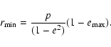
Before we describe our Monte Carlo simulation scheme we present a
very useful method for obtaining the minimum possible perihelion distance
of a comet during its long-term dynamical evolution under the galactic
disk tide. To this aim we use the analytical solution of averaged
equations of a comet motion derived in Breiter et al. (1996).
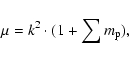
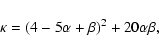
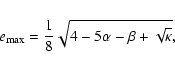
Given the angular momentum vector
![]() and the Laplace vector
and the Laplace vector
![]() of a comet (
of a comet (![]() defined by Eq. (2)), it is easy to calculate
its eccentricity
defined by Eq. (2)), it is easy to calculate
its eccentricity ![]() and parameter
and parameter
![]() .
With auxiliary
variables:
.
With auxiliary
variables:
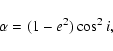
The same formulas as presented above may be used to filter out comets that go too far during their orbit evolution and thence are treated as "lost'' from the cloud. An equivalent criterion may also be derived from the solution proposed by Matese & Whitman (1989), while the formulas proposed by Maciejewski & Pretka (1998) provide a rough estimation only but are thus less effective in this case.
As the main purpose of this paper is to demonstrate the results of
a single stellar passage through or near the Oort cometary cloud under
the simultaneous influence of galactic perturbations, we found it
necessary to separate the sample of comets observable due to the effect
in question from the background of observable comets produced by the
galactic tide alone. We performed such a separation by means of the
dynamical filtering described above. This filter allows us to reject
all comets that can become observable without the stellar action.
In this situation we have a steady state cloud model modified in such
a manner that no comet can be observed under the galactic perturbation
at any time. Then we apply the stellar impulse, which makes some comets
observable without the need of any additional perturbations and, at
the same time, stirs the whole cloud, transferring some other comets
into the region of the phase space from which they might be observable
later due to the disk tide action. This is admittedly a rather artificial
model. It corresponds to the situation where stellar passages are
well separated in time and do not overlap (which is not true in reality)
and all observable comets are removed by planetary perturbations prior
to the stellar passage. However, such a model allows detailed observations
of population of observable comets induced by a single stellar passage
combined with the subsequent Galactic disk tide perturbations. Thus
the ![]() criterion (calculated from Eq. (7)) is used
twice (in opposite ways and with different threshold values) in the
simulation scheme presented below.
criterion (calculated from Eq. (7)) is used
twice (in opposite ways and with different threshold values) in the
simulation scheme presented below.
Our numerical simulation code uses several parameters defining the problem: inner (IB) and outer (OB) boundaries of the cometary cloud, "virgin boundary'' (VB) - the minimum heliocentric distance for which a comet may still be treated as not perturbed by the planets (i.e. it still belongs to the Oort cloud), "lost boundary'' (LB) - the maximum heliocentric distance behind which a comet is treated as lost from the cloud and the observability limit (OL). In all simulations presented in this paper, we used: IB=50 AU, OB= 100 000 AU, VB=15 AU, LB= 150 000 AU, and OL=5 AU.
In our numerical simulation code used to obtain Figs. 5-7, we applied the following scheme:
In simulations performed to obtain results presented in Figs. 2-4, the filtering in Step 4 was omitted; instead some additional initial relaxation of the cometary cloud was added to avoid initial lack of observable comets, visible in Fig. 1 (first 50 mln years).
The effect of planetary perturbations described in Sect. 3 is completely ignored during simulation (except for the indirect account for the past perturbations, Step 4.) and applied only in post-processing (analyzing and plotting) of the data obtained. In the final data sets we record comet orbital elements at each perihelion passage below 15 AU. As a result, at the analysis stage we can apply different values of the "transparency coefficient'' P and different observability limits (5, 3 or 1 AU) without repeating the time-consuming simulation calculations. The only disadvantage to this approach is producing huge output files that contain cometary elements at all perihelion passages below 15 AU.
![\begin{figure}
\par\includegraphics[angle=-90,width=8.8cm,clip]{3327fig2.ps}
\end{figure}](/articles/aa/full/2005/38/aa3327-05/img43.gif) |
Figure 2: The percentage of the observable part of the cometary cloud "refreshed'' by the stellar passage as a function of the perturber velocity and proximity. The upper panel shows results for the DLDW model and the lower one for the DQT model of the cloud. In both cases, stellar mass equals that of the Sun. Curves a, b, c, d, and e describe results for q*=10, 30, 50, 70, and 90 thousand of AU, respectively. Note the different vertical scales of these two panels in this figure and the next one. |
| Open with DEXTER | |
![\begin{figure}
\par\includegraphics[angle=-90,width=8.8cm,clip]{3327fig3.ps}
\end{figure}](/articles/aa/full/2005/38/aa3327-05/img44.gif) |
Figure 3: The fraction of the whole cloud removed (i.e. transfered to the "lost'' state, see text) after the stellar passage. The upper panel shows results for the DLDW model and the lower one for the DQT model of the cloud. Again curves a, b, c, d, and e describe the results for the Sun-star minimal distance d*=10, 30, 50, 70, and 90 thousand of AU, respectively. |
| Open with DEXTER | |
![\begin{figure}
\par\includegraphics[angle=-90,width=8.8cm,clip]{3327fig4.ps}
\end{figure}](/articles/aa/full/2005/38/aa3327-05/img45.gif) |
Figure 4:
Dependence of the removed fraction of the whole
cloud on the mass and velocity of the stellar perturber. The upper
panel shows results for the M*= 3 |
| Open with DEXTER | |
The dynamical filtering described above (see alsoBreiter et al. 1996) may also be used as a tool for examining the overall effect of a stellar passage. Such an approach is very efficient because it is not necessary to integrate any orbits numerically and it gives an overestimation of the size of the observable part of the cloud of only few percent. When applied to DQT and DLDW cometary cloud models, before the stellar passage it gives very similar sizes of the potentially observable part of the cloud under the influence of the galactic disk tide, 6.2% and 6.0% respectively. This means that the probability that a comet will be observable (i.e. the perihelion distance will become lower than the assumed observability limit OL) is on the order of 0.06 if we wait long enough, the period of the long term orbit variations due to the Galactic tide is on the order of 108-1010years.
What is really surprising, after the stellar passage (of any tested mass, velocity, and geometry) the size of this observable part of the cloud remains the same. The only effect of the stellar perturbation is the replacing a small percent of this part with new comets taken from the initially unobservable part. One can observe this effect in Fig. 2 for both cloud models and different stellar velocities and proximity distances. As a result, the probability of being observed does not change due to the stellar passage, the only effect being some asymmetries in apside line direction distributions and variations in the observable cometary influx with time. The remarkable difference between the two cloud model's results comes from the fact that in the DLDW model most comets reside in the outer part of the cloud and are more sensitive to stellar perturbations.
The second result of the stellar perturbation is that a fraction of the whole cometary cloud is lost. Some cometary orbits become hyperbolic, while the aphelion distances of the others become larger than the outer limit of the cloud OL. This fraction of lost comets is different for the two models of the cloud used in this paper, and in both cases it depends on the stellar perturber mass and velocity, see Figs. 3 and 4. Note that even for very strong (and extremely rare) perturbations (large stellar mass with small velocity and deep penetrating passage), this lost fraction does not exceed 10%.
Again the difference between the results obtained for DQT and DLDW models comes from the different structures of these models, shown in detail in Paper I. The DQT model consists of a much more numerous inner part of the cloud, almost immune to stellar perturbations, so the percentage of lost comets is considerably smaller in the case of DQT.
![\begin{figure}
\par\includegraphics[width=11.2cm,clip]{3327fig5.eps} %
%
\end{figure}](/articles/aa/full/2005/38/aa3327-05/img46.gif) |
Figure 5: Results of the numerical simulation of producing observable comets with stellar impulse and galactic disk tide acting simultaneously. The upper part of this figure describes the distribution of the perihelion directions of observable comets on the celestial sphere in the "stellar'' reference frame. The parameters of the star and its passage are shown in the upper left corner. The dashed black line represents the projection of the star heliocentric orbit plane; star perihelion and anti-perihelion directions are marked with full and empty circles, respectively. The continuous black line denotes the position of the galactic disk plane. In the lower part, the obtained observable cometary influx versus time is presented. To be compared directly with Fig. 7 of Paper I. |
| Open with DEXTER | |
![\begin{figure}
\par\includegraphics[width=11.2cm,clip]{3327fig6.ps} %
%
\end{figure}](/articles/aa/full/2005/38/aa3327-05/img47.gif) |
Figure 6: Results of the numerical simulation of producing observable comets with stellar impulse and galactic disk tide acting simultaneously. In this example the output of the strong stellar perturbation with q*=30 000 AU is presented. Because of the high efficiency of such an event, we included two additional copies of the directional distribution of perihelion points for two separate time intervals at the bottom of this figure. High concentration of perihelion points in the first 2 mln years is thus clearly visible. Note the characteristic deficiency of perihelion points near the Galactic equator (solid curve in upper part plot). To be compared directly with Fig. 8 of Paper I. |
| Open with DEXTER | |
![\begin{figure}
\par\includegraphics[width=11.2cm,clip]{3327fig7.eps} %
%
\end{figure}](/articles/aa/full/2005/38/aa3327-05/img48.gif) |
Figure 7: The third example the simulation of producing observable comets with stellar impulse and galactic disk tide acting simultaneously, to be compared directly with Fig. 9 of Paper I. It is the case of rather weak (and the most probable) stellar action for q*= 90 000 AU. The upper plot is presented in the Galactic frame; the straight solid line represents the galactic equator, while the dashed curve represents the heliocentric star orbit plane. In the flux histogram, two consecutive maxima of the same value are clearly shown. The are separated by approx. 9 mln years. A very deep minimum of observable cometary flux occurs 9 mln years after the stellar passage. |
| Open with DEXTER | |
In Paper I we presented three examples of the perihelion direction
distribution of observable comets induced by stellar passages for
![]() 30 000, 60 000, and 90 000 AU. The same three cases
are presented in this paper for a simultaneous stellar and galactic
perturbations model. The corresponding perihelion direction distributions,
as well as the cometary influx time-dependence, are presented in Figs. 5-7. The
format of these pictures is the same as in Paper I: the upper part
presents the equal-area plot of the perihelion direction distribution
on a celestial sphere, while the lower part consists of the histogram
of the observable comet influx versus time. In Fig. 6
there is an additional part of the plot; the perihelion direction
distribution is repeated at the bottom of the figure for two different
time intervals. Because in each simulation we followed numerically
the motion of a comet under the influence of the galactic disk tide
for 20 million years after the stellar passage and checked whether
a comet becomes observable or not, we changed the scale of the horizontal
axis of the flux histograms. To compensate for this (as well as for
the simulated cloud population change for
30 000, 60 000, and 90 000 AU. The same three cases
are presented in this paper for a simultaneous stellar and galactic
perturbations model. The corresponding perihelion direction distributions,
as well as the cometary influx time-dependence, are presented in Figs. 5-7. The
format of these pictures is the same as in Paper I: the upper part
presents the equal-area plot of the perihelion direction distribution
on a celestial sphere, while the lower part consists of the histogram
of the observable comet influx versus time. In Fig. 6
there is an additional part of the plot; the perihelion direction
distribution is repeated at the bottom of the figure for two different
time intervals. Because in each simulation we followed numerically
the motion of a comet under the influence of the galactic disk tide
for 20 million years after the stellar passage and checked whether
a comet becomes observable or not, we changed the scale of the horizontal
axis of the flux histograms. To compensate for this (as well as for
the simulated cloud population change for
![]() 60 000) in
Figs. 5-7,
we also changed the vertical scale so the lower part histograms can
be directly compared with the corresponding plots in Figs. 7-9 of Paper I. The orientations of the upper part plots were also kept
the same. The heliocentric orbit parameters of the stellar perturber
with respect to the Galactic frame are shown in the left upper corner
of each of these figures.
60 000) in
Figs. 5-7,
we also changed the vertical scale so the lower part histograms can
be directly compared with the corresponding plots in Figs. 7-9 of Paper I. The orientations of the upper part plots were also kept
the same. The heliocentric orbit parameters of the stellar perturber
with respect to the Galactic frame are shown in the left upper corner
of each of these figures.
The highly concentrated distributions obtained in all cases in Paper I are spread more in the present model due to the galactic perturbations. But the subsample of comets, observable shortly after the stellar passage, remains concentrated near the anti-perihelion of the star heliocentric orbit in the same manner as in Paper I. It means that if we know the geometry of the stellar passage, we can predict the region of the celestial sphere occupied by the perihelion directions of the observable comets during the first maximum of the flux induced by the stellar perturbation.
In all three examples the flux of observable comets decreases after the first peak (located almost exactly at the same time as in Paper I), then rises again due to the galactic tide perturbations and continues long after the stellar passage. The maximum flux in the first peak appears to be a little smaller in the present model than obtained for the separate stellar perturbation in Paper I. It means that the perihelion distances of some comets placed in the observable part of the cloud, due to the stellar passage, evolve first towards higher values than to the observability limit OL before the first visit among planets and these comets will be observable much later.
It should be noted here that the results presented in Figs. 5-7 are somewhat filtered: in our simulation scheme we removed any potentially observable comets (due to the Galactic tide) from the cometary cloud before the stellar passage occurs. This was done to separate any fingerprints of the stellar perturbation from the background of the comets observable due to the galactic action. As mentioned in the previous section, the overall number of observable comets does not change after the stellar passage, so any stellar fingerprints are limited to the presented asymmetries and variations of the cometary influx with time.
In Paper I we presented distributions of the semi-major axes of the observable comets for three presented examples of stellar passages. They remain almost unchanged in the present model of mixed stellar and galactic perturbation; therefore, we do not present them here and the interested reader is directed to Paper I.
We presented results of simulations of stellar passages through or near the Oort cometary cloud under the simultaneous action of the galactic disk tide. The result of the stellar perturbation for different geometries, masses, and velocities of the perturber and for two different cloud models, is described.
The main conclusions are:
Acknowledgements
The research described in this paper was supported by KBN grant No. 2P03D01324. This manuscript was prepared with LYX, the open source front-end to the TEXsystem.