![[*]](/icons/foot_motif.gif) ,
,
A&A 440, 321-343 (2005)
DOI: 10.1051/0004-6361:20052797
,
K. Jonsell1 - B. Edvardsson1 - B. Gustafsson1 - P. Magain2 - P. E. Nissen3 - M. Asplund4
1 - Department of Astronomy and Space Physics, Uppsala Astronomical
Observatory, Box 515, 751 20 Uppsala, Sweden
2 - Institut d'Astrophysique et de Géophysique, Université de Liège, Allée du 6 Août 17, 4000 Liège, Belgium
3 - Institute of Physics and Astronomy, University of Aarhus,
8000 Aarhus C, Denmark
4 - Research School of Astronomy and Astrophysics, Mount Stromlo
Observatory, Cotter Road, Weston, ACT 2611, Australia
Received 31 January 2005 / Accepted 26 April 2005
Abstract
We have derived abundances of O, Na, Mg, Al, Si, Ca, Sc, Ti, V, Cr, Fe, Ni,
and Ba for 43 metal-poor field stars in the solar neighbourhood, most of
them subgiants or turn-off-point stars with iron abundances [Fe/H] ranging
from -0.4 to -3.0. About half of this sample has not been
spectroscopically analysed in detail before. Effective
temperatures were estimated from uvby photometry, and surface gravities
primarily from Hipparcos parallaxes. The analysis is differential relative
to the Sun, and was carried out with plane-parallel MARCS models.
Various sources of error are discussed
and found to contribute a total error of about 0.1-0.2 dex for most elements,
while relative abundances, such as [Ca/Fe], are most probably more accurate.
For the oxygen abundances, determined in an NLTE analysis of the 7774 Å
triplet lines, the errors may be somewhat larger.
We made a detailed comparison with similar studies and traced the
reasons for the, in most cases, relatively small differences.
Among the results we find that [O/Fe] possibly increases beyond
[Fe/H] = -1.0, though considerably less so than in results obtained by others
from abundances based on OH lines.
We did not trace any tendency toward strong overionization of iron, and
find the excesses, relative to Fe and the Sun, of the  elements Mg,
Si, and Ca to be smaller than those of O. We discuss some indications that
also the abundances of different
elements relative to Fe vary and
the possibility that some of the scatter around the trends in abundances relative
to iron may be real.
This may support the idea that the formation of Halo stars occurred in
smaller systems with different star formation rates. We verify the finding by
Gratton et al. (2003b, A&A, 406, 131) that stars that do not participate in the rotation
of the galactic disk show a lower mean and larger spread in [/Fe]
than stars participating in the general rotation.
The latter stars also seem to show some correlation between [/Fe] and
rotation speed. We trace some stars with peculiar abundances, among these two Ba
stars, HD 17072 and HD 196944,
the second already known to be rich in s elements. Finally we advocate that a
spectroscopic study of a larger sample of halo stars with well-defined
selection criteria is very important, in order to add to the very considerable
efforts that various groups have already made.
elements Mg,
Si, and Ca to be smaller than those of O. We discuss some indications that
also the abundances of different
elements relative to Fe vary and
the possibility that some of the scatter around the trends in abundances relative
to iron may be real.
This may support the idea that the formation of Halo stars occurred in
smaller systems with different star formation rates. We verify the finding by
Gratton et al. (2003b, A&A, 406, 131) that stars that do not participate in the rotation
of the galactic disk show a lower mean and larger spread in [/Fe]
than stars participating in the general rotation.
The latter stars also seem to show some correlation between [/Fe] and
rotation speed. We trace some stars with peculiar abundances, among these two Ba
stars, HD 17072 and HD 196944,
the second already known to be rich in s elements. Finally we advocate that a
spectroscopic study of a larger sample of halo stars with well-defined
selection criteria is very important, in order to add to the very considerable
efforts that various groups have already made.
Key words: stars: Population II - stars: fundamental parameters - stars: abundances - Galaxy: halo - Galaxy: abundances - Galaxy: evolution
More recently, important clues have come from abundance differences
in various stellar populations.
Thus, Gratton et al. (1996, 2000) and Fuhrmann (1998) have traced significant
[/Fe] ratio (i.e., e.g. Mg, Si, and Ca vs. Fe)
differences between the Thick and Thin Galactic disks, suggesting an age
difference between the two systems and a period of little or no star-formation
in between, possibly marking large-scale infall events.
Different kinematic properties at a given [Fe/H]
may be traced in the disk (see also Bensby et al. 2003).
Also two different populations have been traced for the halo stars, as
reflected in kinematic properties and [/Fe] ratios
(Nissen & Schuster 1997; Gratton et al. 2003a,b).
Gratton et al. distinguish between one population with positive velocity
in orbits around the galactic centre and with close correlations
between rotational velocity, metallicity, and [/Fe], and a second
population with small or retrograde orbital velocity with larger scatter in the
abundances.
The star-to-star scatter in relative abundances, such as in
[/Fe] at a given [Fe/H] for halo stars, may also be used to obtain
information on the supernovae, star-formation processes and gas dynamics in the
early Galaxy, since supernovae with different initial masses produce different
relative amounts of the heavy elements (see Nissen et al. 1994;
Karlsson & Gustafsson 2001; Carretta et al. 2002; Arnone et al. 2004;
Cayrel et al. 2004).
In order to study the star-to-star scatter, as well as the possible existence of fine structure in the halo-population and the transition to the thick disk population in terms of abundances and kinematics, the present project was initiated with observations more than a decade ago. About half of our programme stars have been independently studied more recently. Our results give checks or support of results obtained by others and add some significant knowledge for understanding Halo formation.
 photometry and the Olsen (1993) catalogue of
G-dwarfs. The parameters for the stars lie within the following intervals:
photometry and the Olsen (1993) catalogue of
G-dwarfs. The parameters for the stars lie within the following intervals:
 ,
,
 ,
and [Me/H] < -0.4.
The stars all have
,
and [Me/H] < -0.4.
The stars all have
 .
.
The observations were performed in 1987 and 1988 at the ESO 1.4 m Coudé Auxiliary Telescope, CAT, with the short camera of the Coudé Echelle Spectrometer, CES, equipped with the RCA CCD No. 9. The setup made it possible to obtain a spectral resolving power of 60 000 and a signal to noise ratio over about 200. To get a reasonably large sample of unblended lines of important elements four different wavelength regions were observed: 5670-5720, 6120-6185, 7750-7820, and 8710-8780 Å.
The CCD used in the programme, RCA No. 9, was not fully linear at the time of
observation, as found by one of us in a careful analysis including simulations
of the effects on measured equivalent widths (Gosset & Magain 1993).
To correct for this nonlinearity our equivalent widths, W,
were reduced:
Up to 62 usable absorption lines were measured. For infrared lines with
equivalent widths under 40 mÅ, the widths were measured with a Gaussian fit.
Lines stronger than this were fitted with a Voigt profile. Lines in the visual
region of the stellar spectra were measured by a weighted mean between a
Gaussian fit and a pure numerical integration.
The weighting was estimated by eye
with respect to suspected blends, line strength, etc.
The widths for HD 140283 and HD 196944 in the 7780 Å
region are the averages for two spectra.
In Fig. 1 we compare our equivalent widths for 212 lines with
measurements by Gratton et al. (2003a).
The mean difference (Us-Gratton et al.) is +0.1 mÅ with a standard
deviation of 3.2 mÅ.
![\begin{figure}
\par\includegraphics[width=8.6cm,clip]{2797F01.eps}
\end{figure}](/articles/aa/full/2005/34/aa2797-05/img20.gif) |
Figure 1: Comparison of equivalent width measurements with those of Gratton et al. (2003a). The dotted line indicates the 1-to-1 relation. |
| Open with DEXTER | |
Table 2: Data for the 43 stars in the project. Column 1: stellar identification. Column 2: visual apparent magnitude. Column 3: colour index(b-y). Column 4: balmer discontinuity index c1. Column 5: references for the photometry: 1) Olsen (1983), 2) Schuster & Nissen (1988), 3) Lindgren H. (unpublished), 4) Olsen (1993), 5) Hauck & Mermilliod (1998), 6) Grønbech & Olsen (1976, 1977), 7) SIMBAD. Columns 6-8: stellar space velocities relative to the LSR, see Sect. 3.2. Column 9: stellar masses in units of the Solar mass, see Sect. 3.1.2. Column 10: the effective temperatures. except for HD 196944. Column 11: the metallicities determined from spectroscopy, see Sect. 3.1.2. Column 12: gravitational parameters from Hipparcos parallaxes and evolutionary tracks (VandenBerg et al. 2000), except for HD 196944. Column 13: the classification of the stars according to the SIMBAD database. Column 14: Ba = barium star, b = binary (Nordström et al. 2004), b? = possible binary (Nissen et al. 1997), v = variable (Cayrel de Strobel et al. 1997).
Effective temperatures.
 values for the programme stars were
derived from Strömgren
photometry collected from
sources given in the table caption.
The empirical temperature calibration of Alonso et al. (1996; their Eq. (9))
was used to estimate the effective temperatures.
This calibration is based on the InfraRed Flux Method, a grid of Kurucz'
atmosphere models and a large sample of dwarfs and subdwarfs in the metallicity
range
values for the programme stars were
derived from Strömgren
photometry collected from
sources given in the table caption.
The empirical temperature calibration of Alonso et al. (1996; their Eq. (9))
was used to estimate the effective temperatures.
This calibration is based on the InfraRed Flux Method, a grid of Kurucz'
atmosphere models and a large sample of dwarfs and subdwarfs in the metallicity
range  [Fe/H]
  .
In applying the calibration we iterated until consistency was achieved between
the calculated temperatures, the metallicities, the surface gravities and the
derived iron abundances of the stars.
The effective temperature of the star HD 196944 was adopted from
Zacs et al. (1998).
The reddening was calculated for all stars from H
.
In applying the calibration we iterated until consistency was achieved between
the calculated temperatures, the metallicities, the surface gravities and the
derived iron abundances of the stars.
The effective temperature of the star HD 196944 was adopted from
Zacs et al. (1998).
The reddening was calculated for all stars from H ,
and was
found to be small for all stars but one, so reddening was
neglected in the analysis (see Sect. 5.2, below).
,
and was
found to be small for all stars but one, so reddening was
neglected in the analysis (see Sect. 5.2, below).
Metallicities. The overall metallicities, [Me/H], of the stars were first approximated by using a calibration of Strömgren photometry made by Schuster & Nissen. The metallicities were changed until consistency was achieved with the derived iron abundances, [Fe/H], from lines of Fe I, the surface gravities and the effective temperatures.
Surface gravities.
Values of  were calculated from Hipparcos parallaxes
in the same way as described by Nissen et al. (1997) in their Eq. (3).
An age of 14 Gyr was assumed for all stars.
The stellar masses were estimated from the evolutionary tracks of
VandenBerg et al. (2000).
For some stars, that were not faint enough for these tracks, 0.80
were calculated from Hipparcos parallaxes
in the same way as described by Nissen et al. (1997) in their Eq. (3).
An age of 14 Gyr was assumed for all stars.
The stellar masses were estimated from the evolutionary tracks of
VandenBerg et al. (2000).
For some stars, that were not faint enough for these tracks, 0.80  was adopted.
Some stars were located on the lower side of the track, and some stars resided
in the crowded part of the giant branch.
In these cases, the masses will have higher uncertainties.
The visual magnitudes were adopted from different sources, the bolometric
corrections were determined from Alonso et al. (1995), and the parallaxes
adopted
from the Hipparcos catalogue (ESA 1997). The temperatures, metallicities,
iron abundances, and gravities were iterated until consistency was achieved.
The surface gravity of the star HD 196944 was set to
was adopted.
Some stars were located on the lower side of the track, and some stars resided
in the crowded part of the giant branch.
In these cases, the masses will have higher uncertainties.
The visual magnitudes were adopted from different sources, the bolometric
corrections were determined from Alonso et al. (1995), and the parallaxes
adopted
from the Hipparcos catalogue (ESA 1997). The temperatures, metallicities,
iron abundances, and gravities were iterated until consistency was achieved.
The surface gravity of the star HD 196944 was set to
 according to Zacs et al. (1998).
Microturbulence parameters.
 represents the doppler broadening
of the lines by non-thermal small-scale motions in the stellar atmosphere.
Here the microturbulence parameter was set to
represents the doppler broadening
of the lines by non-thermal small-scale motions in the stellar atmosphere.
Here the microturbulence parameter was set to
 km s-1.
A microturbulence parameter of 1.9 km s-1 was adopted from Zacs et al. (1998)
for the star HD 196944.
km s-1.
A microturbulence parameter of 1.9 km s-1 was adopted from Zacs et al. (1998)
for the star HD 196944.
 ,
,
 and
and
 km s-1 of Dehnen & Binney (1998).
![\begin{figure}
\par\includegraphics[width=8.6cm,clip]{2797F02.eps}
\end{figure}](/articles/aa/full/2005/34/aa2797-05/img34.gif) |
Figure 2:
A Toomre diagram for the stars, where the symbols have been coded
according to the overall stellar metallicity:
-1.0  [Fe/H] (crosses), -1.5 [Fe/H] < -1.0 (open circles),
and [Fe/H] < -1.5 (filled circles). The curves connect loci with identical
total velocities relative to the LSR.
The diagram shows an obvious anticorrelation between overall metallicity and
total LSR velocity. [Fe/H] (crosses), -1.5 [Fe/H] < -1.0 (open circles),
and [Fe/H] < -1.5 (filled circles). The curves connect loci with identical
total velocities relative to the LSR.
The diagram shows an obvious anticorrelation between overall metallicity and
total LSR velocity. |
| Open with DEXTER | |
Figure 2 shows the kinematic Toomre diagram for our sample and displays the well-known relation between overall metallicity and velocity relative to the local standard of rest.
The lines chosen were selected to be essentially free of blends. Since most lines are weak both in the solar and stellar spectra, the effects on the equivalent widths by isotope splitting (IS) and hyperfine-structure splitting (hfs) should not be important. The exception may be the Ba II line (at 6141.71 Å), which is blended with a line of Fe I and which shows both hfs and IS. For this line we made detailed synthetic-spectrum calculations with the programme BSYN, a sister programme to EQWIDTH, taking the iron-line blend and the different line components into consideration with hfs and IS data from McWilliam (1998) and assuming solar isotope ratios. We found, however, that the IS and hfs splittings are negligible for this line.
The oxygen IR triplet lines, used here for determining the oxygen abundances, are known to be severely affected by departures from LTE (e.g. Kiselman 1991, 1993; Nissen et al. 2002). We have therefore solved the statistical-equilibrium equations for an oxygen model atom with 23 levels and 65 radiative transitions, kindly provided by Dan Kiselman. For method and atomic data; see Nissen et al. (2002). These calculations were made individually for each star with appropriate model atmospheres. The corrections in abundances range from -0.07 to -0.33 dex and barely seem affected by the uncertainties in hydrogen-collision cross sections (cf. Nissen et al. 2002).
 ,
excitation energies
,
excitation energies
 ,
and radiation damping constants
,
and radiation damping constants
 .
For some lines of sodium, magnesium and silicon VALD had no radiation damping
constants listed, so they were then taken from the tables of Kurucz (1989).
For the barium line the radiation damping
constant was calculated from lifetimes of relevant energy levels identified
in the tables of Bashkin & Stoner (1975).
The line data are given in Table 3 which is only available in electronic form.
.
For some lines of sodium, magnesium and silicon VALD had no radiation damping
constants listed, so they were then taken from the tables of Kurucz (1989).
For the barium line the radiation damping
constant was calculated from lifetimes of relevant energy levels identified
in the tables of Bashkin & Stoner (1975).
The line data are given in Table 3 which is only available in electronic form.
 values
by running the analysis programme EQWIDTH with known abundances, solar-flux
equivalent widths, and a solar model atmosphere.
The photospheric solar abundances,
values
by running the analysis programme EQWIDTH with known abundances, solar-flux
equivalent widths, and a solar model atmosphere.
The photospheric solar abundances,
 (Table 3), were adopted from
Grevesse & Sauval (1998) with the exception of oxygen for which
the abundance of Asplund et al. (2004) was adopted.
A MARCS model was used with the parameters
(Table 3), were adopted from
Grevesse & Sauval (1998) with the exception of oxygen for which
the abundance of Asplund et al. (2004) was adopted.
A MARCS model was used with the parameters
 K,
K,
 dex, [Fe/H] = 0.00 dex, and
 km s-1.
For the oxygen triplet lines, corrections for NLTE (-0.22 dex) were
applied when determining the gf values.
km s-1.
For the oxygen triplet lines, corrections for NLTE (-0.22 dex) were
applied when determining the gf values.
The choice of a differential analysis relative to the Sun may not be optimal in our case. The stars depart systematically from the Sun in one important respect: they are more metal-poor so their lines from heavy elements are generally weaker. Also, the choice of a MARCS model is not obvious. True enough, errors may cancel if one chooses the Solar model from the same grid as for the programme stars; however, this cancellation may be only partial since, the programme stars are systematically different. Therefore, arguments for adopting a semi-empirical solar model instead can be raised; cf. Sect. 5.6.3.
Table 4:
Spectroscopic metallicities [Fe/H]
 ,
and abundances relative to iron [X/Fe]
,
derived for 13 neutral and ionized species X.
For oxygen, NLTE corrections were applied:
[/Fe] =
,
and abundances relative to iron [X/Fe]
,
derived for 13 neutral and ionized species X.
For oxygen, NLTE corrections were applied:
[/Fe] =
![$\frac{1}{4}({\rm [Mg/Fe]}+
{\rm [Si/Fe]}+{\rm [Ca/Fe]}+{\rm [Ti/Fe]})$](/articles/aa/full/2005/34/aa2797-05/img44.gif) ,
and ['/Fe] =
,
and ['/Fe] =
![$\frac{1}{3}({\rm [Mg/Fe]}+{\rm [Si/Fe]}+{\rm [Ca/Fe]})$](/articles/aa/full/2005/34/aa2797-05/img45.gif) .
.
![\begin{figure}
\par\includegraphics[width=14cm,clip]{2797F03.eps}
\end{figure}](/articles/aa/full/2005/34/aa2797-05/img49.gif) |
Figure 3:
The abundances relative to iron [X/Fe]
 for all species in the
programme as a function of the iron abundance with addition of the data of
Edvardsson et al. (1993) as small dots.
For species where Edvardsson et al. have no data (Sc I, V I and
Cr I) the data of Reddy et al. (2003) is shown instead.
Note the different ordinate scale in panel m).
In panel n) the circles denote
[/Fe]
for all species in the
programme as a function of the iron abundance with addition of the data of
Edvardsson et al. (1993) as small dots.
For species where Edvardsson et al. have no data (Sc I, V I and
Cr I) the data of Reddy et al. (2003) is shown instead.
Note the different ordinate scale in panel m).
In panel n) the circles denote
[/Fe]
![$=\frac{1}{4}({\rm [Mg/Fe]}+{\rm [Si/Fe]}+
{\rm [Ca/Fe]}+{\rm [Ti/Fe]})$](/articles/aa/full/2005/34/aa2797-05/img47.gif) ,
and the crosses
['/Fe] ,
and the crosses
['/Fe]
![$=\frac{1}{3}({\rm [Mg/Fe]}+{\rm [Si/Fe]}+{\rm [Ca/Fe]})$](/articles/aa/full/2005/34/aa2797-05/img48.gif) for
stars with no Ti abundance determinations.
for
stars with no Ti abundance determinations. |
| Open with DEXTER | |
The solar equivalent widths were measured from a computer-readable version of the atlas of Kurucz et al. (1984). The lines were fitted twice with the programme package IRAF: with a Gaussian fit and alternately by a numerical integration. The final width was set as a weighted mean of these values, with the weighting determined by visual inspection.
When determining the gf value of the Ba II 6141.713 Å line, which
has an Fe I blend, we first scaled the iron line gf value to two other
lines of the same multiplet, 6232.5 and 6302.5 Å, which were fitted to the
solar flux atlas of Kurucz et al. (1984).
The relative scaling was based on the gf values listed by Bard et al. (1991),
and the fitting of the two lines resulted in increased
values
by +0.02 and +0.10 dex, respectively.
The adopted
value of the Fe I is -1.40; 0.06 dex higher than
given by Bard et al.
Synthesis of the Ba II line, including the (negligible) hfs and IS
splittings and the Fe I line to the solar atlas, indicated that the Ba
and Fe lines do not differ in central wavelengths by more than 0.005 Å.
Therefore these wavelengths were set to be identical.
Finally, requiring the total equivalent width of the blend to be equal to our
measured solar equivalent width resulted in a
for the Ba II
line of -0.13, which is 1.1  lower than the NBS value of -0.077(Wiese & Martin 1980).
-element behaviour'' of Mg, Si, Ca, and possibly of
Ti, with a rise of [X/Fe] as one proceeds towards the more metal-poor
stars, and a levelling off to a plateau for [Fe/H] < -1.
It is not clear, however, that this plateau level is strictly horizontal, a
question which will be discussed in Sect. 6.
Also, O shows similar behaviour.
We saw "iron-like'' behaviour of Ni and possibly Cr, with [X/Fe] staying
close to solar also for metal-poor stars.
We found that the "odd-Z element'' Al behaves like the
even-Z alpha elements (cf. Si!), while the odd Na behaves differently.
We find that Sc, V, and Ba do not show any clear rise relative to Fe with
decreasing [Fe/H] and that the [Ba/Fe] ratio (based on only one blended feature)
shows a substantial scatter, seemingly caused by some pronounced outliers.
In all panels of Fig. 3 where our data overlap with the disk star
data there is a smooth transition between the data sets.
One important question is if the scatter around the mean trends in Fig. 3 are real or caused by errors in the analysis; e.g., is the increased scatter, when we proceed to stars with [Fe/H] < -1.0, visible for most elements, due to a real spread in abundances or caused by weaker and fewer measurable lines, lower S/N, or more uncertain fundamental parameters? Do the differences in scatter, ranging from 0.03 dex (in [Ca/Fe]) to above 0.1 dex (e.g. in [O/Fe], [Al/Fe], [Ba/Fe]) around the mean relations, tell us anything about nucleosynthesis? Is any of the scatter in the alpha elements [Si/Fe] and [Mg/Fe] real, in view of the smaller scatter in [Ca/Fe] at a given [Fe/H]? Discussion of such questions will be postponed until after both the error discussion in Sect. 5 and a detailed comparison with results from other studies in Sect. 6.
One additional feature of Fig. 3 should be pointed out - the nice agreement in iron abundances as derived from the Fe I lines and the (single!) Fe II line. This agreement will also be further discussed in Sect. 6.
 [X/H]
[X/H]
 were thus calculated for all iron and
nickel lines included in the programme; see Fig. 4. Some
lines did give systematically different abundances from the mean abundance of
the species, and the Ni line 7788 Å was removed from the abundance
determinations altogether.
The reason for the deviating abundances from individual lines
could be due to hidden blends in the Sun, and therefore erroneous
values, or hidden blends or departures from LTE in the stellar spectra depending
on the parameters.
were thus calculated for all iron and
nickel lines included in the programme; see Fig. 4. Some
lines did give systematically different abundances from the mean abundance of
the species, and the Ni line 7788 Å was removed from the abundance
determinations altogether.
The reason for the deviating abundances from individual lines
could be due to hidden blends in the Sun, and therefore erroneous
values, or hidden blends or departures from LTE in the stellar spectra depending
on the parameters.
![\begin{figure}
\par\includegraphics[width=8.8cm,clip]{2797F04.eps}
\end{figure}](/articles/aa/full/2005/34/aa2797-05/img53.gif) |
Figure 4: A consistency check of the abundances of iron ( left) and nickel ( right). The open black circles mark the measurements for each line for each star and the thick (+):s mark the mean for individual lines. For nickel the filled grey circles and the thick ( x):s mark the measurements with the line 7788 Å included. This line was later removed from the analysis due to suspected blending. |
| Open with DEXTER | |
Some silicon lines (6125, 6142, 6145, and 6155 Å) come from double, not single, electron transitions in the atoms. We checked whether these lines behaved differently compared to the rest, but they did not differ more than expected statistically.
Table 5:
The mean abundance effects of changes in effective temperature, surface
gravity, metallicity, and microturbulence.
The last two columns show the abundance change if the -values were
calculated with only the Unsöld approximation, see Sect. 5.6.1
or based on the Holweger & Müller model, see Sect. 5.6.3.
photometry.
However, the mean error in the estimates from the model is typically 0.05 mag.
We conclude that reddenings of typically 0.01 mag
may affect many of our programme stars, leading to underestimates
of effective temperature by about 50 K and of metal abundances
of about 0.03 dex. For a few stars like HD 132475, there
may be more serious underestimates, by even somewhat more than 0.1 dex.
A test was made to investigate the impact of the temperature errors.
Alonso et al. (1996) estimate a standard deviation of 110 K in the effective
temperatures.
Here the parameters were changed  100 K for all stars.
The changes of the chemical abundances were at a mean
100 K for all stars.
The changes of the chemical abundances were at a mean
 dex, but for O I, Ca I, Ti I, V I,
Fe I, and Ba II the mean abundances changed by more than
0.07 dex, see Table 5.
Thus, errors in the effective temperatures have considerable impact on the
result.
dex, but for O I, Ca I, Ti I, V I,
Fe I, and Ba II the mean abundances changed by more than
0.07 dex, see Table 5.
Thus, errors in the effective temperatures have considerable impact on the
result.
A frequently used consistency test of the effective temperatures is to check if the derived abundances are dependent on the excitation energies for the lower states of the lines. The level populations depend on the temperatures through the Boltzmann distribution in the LTE approximation. The numerous lines of Fe I and Ni I with wide ranges both in excitation energy and equivalent widths were selected for these consistency checks. The use of both species together was motivated by the similarities between the elements and the gain in statistics with as many lines as possible.
For each star included in the tests a diagram was plotted to display the
abundance from each line minus the derived mean abundance for the star,
[X/H]
[X/H]
,
versus the excitation energy of the
lower level of the line,
;
see Fig. 5 top
panel. To all diagrams a linear fit was sought, and these slopes were then
plotted in a new diagram with the effective temperatures of the stars on the
abscissa, see Fig. 6.
The check shows that the test is very dependent on the lines employed in the test. If all lines except Ni I 7788 Å are included, the test suggests that the adopted effective temperatures are about 100 K too low for the stars in the lower temperature region and about 25 K too high at high temperatures (thick black line). However, if lines deviating by more than 0.1 dex from the mean in Fig. 4 are removed (removal of the iron lines at 5687 and 8757 Å), the temperatures of the low-temperature stars seem underestimated by some 20 K, while the warmer stars have their temperatures overestimated by about 120 K (thin black line). If spectral lines deviating by more than 0.05 dex are removed (removal of the iron lines at 5687, 5701, 5717, 6136, 6137, 6157, 6170, 7780, 8757, and 8763 Å), then adopted effective temperatures of the low-temperature stars are about 70 K too high and high temperature stars have temperatures about 130 K too low (thick grey line). The conclusion is that this test, assuming that the LTE approximation is valid, suggests that the errors in temperature are not larger than 150 K. For a few stars the temperatures may, however, be underestimated by even more, due to reddening. More precise conclusions cannot be drawn.
 km s-1 for all stars.
The average change of the mean abundances were only
km s-1 for all stars.
The average change of the mean abundances were only  dex. An
exception was barium, for which the change was
dex. An
exception was barium, for which the change was  dex.
dex.
![\begin{figure}
\par\includegraphics[width=8.8cm,clip]{2797F05.eps}
\end{figure}](/articles/aa/full/2005/34/aa2797-05/img60.gif) |
Figure 5: An example of consistency diagrams for an individual star, in this case HD 126793. Filled circles represent iron lines and open circles nickel lines. Linear fits were made to the data for individual stars, and the derived slopes were studied as functions of stellar parameters, e.g., in Fig. 6. |
| Open with DEXTER | |
![\begin{figure}
\par\includegraphics[width=8.8cm,clip]{2797F06.eps}
\end{figure}](/articles/aa/full/2005/34/aa2797-05/img61.gif) |
Figure 6: A consistency check for the effective temperatures. Filled circles and thick black line: all lines included. Squares and black line: the lines 5687 and 8757 Å were removed. Grey triangles and grey line: the lines at 5687, 5701, 5717, 6136, 6137, 6157, 6170, 7780, 8757, and 8763 Å were removed. |
| Open with DEXTER | |
We also checked if the adopted value of 1.5 km s-1 for all stars (except for
HD 196944) give consistent results by investigating whether the line
strengths,
 ,
and the relative abundances
of the lines, [X/H]
[X/H]
,
are correlated.
,
and the relative abundances
of the lines, [X/H]
[X/H]
,
are correlated.
 represents the width the line would have if the mean abundance
from all lines is adopted, following Magain (1984).
If the assumed microturbulence parameter and the underlying line-formation
theory are correct, the relative abundances derived from the individual lines
would be independent of line strength.
represents the width the line would have if the mean abundance
from all lines is adopted, following Magain (1984).
If the assumed microturbulence parameter and the underlying line-formation
theory are correct, the relative abundances derived from the individual lines
would be independent of line strength.
The test was performed in a way similar to that for the effective temperature;
Sect. 5.2. A diagram was plotted for each star with the relative
abundance, [X/H]
[X/H]
,
on the ordinate and the
theoretical line strength,
,
on the
abscissa, see the lower panel of Fig. 5. To all figures a
linear fit was sought.
The results show again that this kind of test is heavily dependent on which lines are included, although one may conclude that the microturbulences are slightly overestimated in general and not optimal for some stars. This has, however, very little impact on the derived mean elemental abundances, with the exception of barium, as discussed in Sect. 6.8.
The metallicities of the model atmospheres were changed 0.5 dex for all
stars.
The change of the mean abundances were on average 0.02 dex, but
higher for Sc II, Fe II and Ba II, as seen in
Table 5.
The conclusion is that errors in the metallicities do not have a large impact.
The derived iron abundances are compared with metallicities given by the
Schuster & Nissen (1989) calibration of Strömgren photometry
in Fig. 7.
Note that the correction to Magain's (1987, 1989) [Fe/H] scale was not
applied - as this scale was found by Gosset & Magain (1993) to be affected
by a non-linear detector.
The derived abundances differed from the photometric ones by
-0.01 dex on average with a standard deviation of 0.25 dex, a maximum
difference of 1.01 dex (HD 91121, with photometry from a separate
source) and a minimum difference of -0.58 dex (HD 196944,
supergiant).
If we remove the 2 outliers,
the mean difference does not change and the equation of the black line is
![\begin{figure}
\par\includegraphics[width=8.8cm,clip]{2797F07.eps}
\end{figure}](/articles/aa/full/2005/34/aa2797-05/img65.gif) |
Figure 7: Comparison of derived iron abundances, [Fe/H], with metallicities from Strömgren photometry obtained from the calibration of Schuster & Nissen (1989). The solid line shows Eq. (2) and the dotted line indicates the 1-to-1 relation. |
| Open with DEXTER | |
0.3 dex.
Our neglect of interstellar absorption may make our assumed reddening-free
V magnitudes too large.
Using the result from Sect. 5.2 above, we estimate that typical
 values hardly exceed 0.04 mag for most stars, and not 0.4 mag for any
of them.
This corresponds to overestimates in
by 0.02 to 0.16 dex,
respectively.
We have compared our gravity estimates with those obtained from Strömgren
photometry and the isochrones of VandenBerg & Bell (1985).
The results agree very well with those obtained here
from the Hipparcos parallaxes. We thus find a relation
values hardly exceed 0.04 mag for most stars, and not 0.4 mag for any
of them.
This corresponds to overestimates in
by 0.02 to 0.16 dex,
respectively.
We have compared our gravity estimates with those obtained from Strömgren
photometry and the isochrones of VandenBerg & Bell (1985).
The results agree very well with those obtained here
from the Hipparcos parallaxes. We thus find a relation
 dex are excluded,
the standard deviation diminishes to 0.11 dex
(cf. Fig. 8).
From these considerations, it seems reasonable to adopt an uncertainty on
the order of 0.2 dex for our estimates of surface gravity parameters.
The effects of these errors on the final element abundances were explored.
The change of the elemental abundances were only 0.02 dex,
but for the elements O I, Sc II, Fe II, and
Ba II, the changes were larger, from 0.04 to 0.08 dex,
respectively, see Table 5.
dex are excluded,
the standard deviation diminishes to 0.11 dex
(cf. Fig. 8).
From these considerations, it seems reasonable to adopt an uncertainty on
the order of 0.2 dex for our estimates of surface gravity parameters.
The effects of these errors on the final element abundances were explored.
The change of the elemental abundances were only 0.02 dex,
but for the elements O I, Sc II, Fe II, and
Ba II, the changes were larger, from 0.04 to 0.08 dex,
respectively, see Table 5.
![\begin{figure}
\par\includegraphics[width=8.8cm,clip]{2797F08.eps}
\end{figure}](/articles/aa/full/2005/34/aa2797-05/img69.gif) |
Figure 8:
Comparison between
from Hipparcos and
Strömgren photometry (see text).
The filled circles and black line represent stars and fits with reliable data
from Strömgren photometry, and squares more indicate uncertain measurements.
The grey line shows a fit to all data. The dotted line shows the 1-to-1
relation. |
| Open with DEXTER | |
values became on the mean
0.03 dex higher with a maximum of +0.26 dex.
The mean abundances of the stellar sample changed very little as seen in
Table 5, but for stars with few measured lines of some
element the effect may be important.
values, counteracting the effects of our higher solar
equivalent widths.
Except for the O I triplet lines, for which Edvardsson et al. did not
make any NLTE corrections, the mean difference in (us-Edvardsson et al.) is 0.02 dex with a standard deviation of 0.05 dex
for the 28 lines in common.
The error in the gf values deduced for the blended Ba II line at
6141 Å depends on the strength adopted for the blending Fe I
line.
If the latter line is totally neglected, we find that the gf value for the
Ba II line increases to
 ,
and the typical Ba
abundances for the programme stars decrease by 0.15 dex.
An increase of the gf value of the Fe I line by 0.2 dex cannot be
excluded, which leads to (Ba II) =-0.30, and
to a typical increase of the Ba abundances by 0.13 dex.
,
and the typical Ba
abundances for the programme stars decrease by 0.15 dex.
An increase of the gf value of the Fe I line by 0.2 dex cannot be
excluded, which leads to (Ba II) =-0.30, and
to a typical increase of the Ba abundances by 0.13 dex.
values for the lines in the programme.
The
values then became 0.11 dex higher on the mean compared to the
ones from a MARCS solar model, with a maximum difference of +0.20 dex.
The stellar abundances decreased by 0.03 dex to 0.15 dex, with
a mean of 0.10 dex for all species, see Table 5.
Although we chose a strictly differential approach in this work, with a solar model from the same grid as the model atmospheres representing the stars, this choice was not obvious, see Sect. 3.3.4. The HM model is known to represent solar limb-darkening and fluxes quite well, and in fact more successfully than theoretical flux-constant 1D models (cf. Blackwell et al. 1995; Gehren et al. 2001; Edvardsson et al., in preparation). Thus, there are reasons to believe that the gf values derived from that model might be better in absolute terms. The cancellation argument, founded on the expectation that systematic errors in the stellar model atmospheres act in similar ways in the solar analysis, is of uncertain weight. Thus, systematic errors in abundances [X/H] of about 0.15 dex are possible. The corresponding errors in abundances relative to iron are smaller; [X/Fe] are on the mean 0.05 dex higher when derived with the HM model (oxygen not included).
values from VALD were on average only 0.04 dex lower compared
to the ones used in the programme, but the maximum difference
(us-VALD) was as large as 2.15 dex (the Fe I line 7780.552 Å) and the
minimum -0.60 dex.
The difference (us-VALD) for neutral iron alone was on the mean -0.48 dex,
with a spread as large as 0.99 dex.
This of course had a large impact on the abundances derived, especially for
species measured with only one line.
A larger spread and sometimes a different form of the abundance trends in the
diagrams could be seen.
We believe that although the use of astrophysical
values has
drawbacks - they depend on the solar model atmosphere, the damping, and on
errors introduced in the measurement of equivalent widths - they are still
to be preferred in a differential analysis.
,
will be underestimated.
The error in the
may amount to 0.3 dex. Also, there may be some
error in the adopted effective temperature, as well as in the metallicity.
None of our spectra show line doubling, which would be an obvious reason
for exclusion from the sample.
We estimate that the abundances for only a few stars should be
significantly affected with abundance errors in excess of 0.05 dex as a
result of binarity.
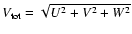 ,
are estimated to be less than 20 km s-1 for
all but ten stars
which all have V velocities lagging behind the LSR by more than 90 km s-1,
,
are estimated to be less than 20 km s-1 for
all but ten stars
which all have V velocities lagging behind the LSR by more than 90 km s-1,
 larger than 160 km s-1, and metallicities less than
[Fe/H] = -1.2.
Another seven stars have uncertainties between 10 and 20 km s-1.
The major source of these errors is uncertain parallax values, while the
radial-velocity errors are negligible.
larger than 160 km s-1, and metallicities less than
[Fe/H] = -1.2.
Another seven stars have uncertainties between 10 and 20 km s-1.
The major source of these errors is uncertain parallax values, while the
radial-velocity errors are negligible.
A special case is oxygen. Here, effective-temperature errors and errors in the gravity may possibly add up to about 0.15 dex. Since the temperature scale may be systematically in error, this may lead to systematically erroneous abundances by, say, 0.1 dex. In addition to that, there may be errors caused by oversimplified model atmospheres, notably the assumption of plane-parallel stratification. We note that García Pérez et al. (2005) find systematic deviations for metal-poor subdwarfs between abundances from O I triplet lines and [O I] lines of typically 0.2 dex and ascribe these differences to errors in the abundances derived from the triplet lines.
We have compared our results with those of a number of recent studies which have some stars in common with ours. The results of these comparisons are displayed in Table 6.
Table 6: Comparison between our abundance results and those of others for stars in common, including the numbers of stars, the mean differences, and standard deviations. Sources: B: Burris et al. (2000), BG: Baumüller & Gehren (1997), F: Fuhrmann (1998), Ge: Gehren et al. (2004), Gr: Gratton et al. (2003a), J: Jehin et al. (1999),MG: Mashonkina & Gehren (2001), McW: McWilliam (1998), N: Nissen et al. (2002), NS: Nissen & Schuster (1997).
Although these studies all share a number of basic features (basically similar model assumptions), they deviate partly in terms of details, such as temperature calibrations, gf values, and model atmospheres. We therefore note with satisfaction that the mutual agreement for stars in common is good. We shall now comment more specifically on our results as compared with those of others.
As is clear from Sect. 5.4 above, we find little evidence of
departures from the Boltzmann excitation equilibrium, in contrast with the
empirical results of Magain & Zhao (1996), who
adopted gf values for the lower excitation iron lines
from Blackwell et al. (1995). For the higher excitation lines, however,
they derive gf values from fitting observed solar-disk centre equivalent
widths to the HM model, adopting a relatively
high solar abundance (
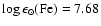 ).
As these authors note, a systematic lowering of the solar
abundance of iron to a value around 7.5, as we have chosen, would nearly
cancel their excitation-equilibrium effect for the metal-poor stars, while
consistency with a standard LTE analysis with the HM model would not be
obtained.
).
As these authors note, a systematic lowering of the solar
abundance of iron to a value around 7.5, as we have chosen, would nearly
cancel their excitation-equilibrium effect for the metal-poor stars, while
consistency with a standard LTE analysis with the HM model would not be
obtained.
As may be seen from Table 6 and Fig. 9,
we find overall agreement in iron abundances
with Nissen et al. (2002), Gratton et al. (2003a), and Jehin et al. (1999).
The abundances of Nissen et al. were based on about 10 Fe II lines,
while those of
Gratton et al. are, at least to a great extent, based on Fe I lines.
The star with the largest departure by far in the comparison with
Gratton et al. is HD 140283, for which we
find considerably higher effective temperature, which explains parts of
the difference. The second largest departure occurs
for HD 84937, the hottest star in our sample.
![\begin{figure}
\par\includegraphics[width=7.5cm,clip]{2797F09.eps}
\end{figure}](/articles/aa/full/2005/34/aa2797-05/img122.gif) |
Figure 9: Comparison of iron abundances derived from Fe I lines with those of Jehin et al. (1999) (squares) and Gratton et al. (2003a) (dots). The differences relative to abundances from lines of Fe II of Nissen et al. (2002) are shown by crosses. |
| Open with DEXTER | |
Jehin et al. (1999) used Fe I lines to derive [Fe/H] abundances differentially relative to HD 76932, for which a metallicity of [Fe/H] = -0.91 was derived from laboratory gf values (our value for this star is -0.89). They also derived iron abundances from Fe II lines; for the 13 stars we have in common their mean value of [Fe/H] from Fe II is -0.02 dex lower than that obtained from the Fe I lines, i.e. no signs of over-ionisation, also consistent with our result.
We also have 13 stars (to some extent the same stars as in the Jehin et al.
study) in common with the earlier study of Zhao & Magain (1991).
Our values of [Fe/H] depart systematically from those of Zhao & Magain by,
on the mean, as much as +0.19 dex.
This difference may be ascribed to the choice of gf values and
solar iron abundance of Zhao & Magain; they use the HM model to derive gf
values for the higher excitation lines and adopt a solar iron abundance,
 ,
of 7.66.
Differences between the results of the studies by
Zhao & Magain (1991) and Jehin et al. (1999) reflect a basic uncertainty
in the solar analysis of iron.
,
of 7.66.
Differences between the results of the studies by
Zhao & Magain (1991) and Jehin et al. (1999) reflect a basic uncertainty
in the solar analysis of iron.
 dex higher when the Kurucz models
are used than for MARCS models, which agrees with our own estimates.
Also, there are differences in stellar parameters.
For the five stars in common between the two studies our
temperatures are on average
dex higher when the Kurucz models
are used than for MARCS models, which agrees with our own estimates.
Also, there are differences in stellar parameters.
For the five stars in common between the two studies our
temperatures are on average  K lower than the King
temperature scale, and
K lower than the King
temperature scale, and  K higher than the Carney scale.
Our gravity parameters and metallicities are very similar, as are the
observed equivalent widths.
K higher than the Carney scale.
Our gravity parameters and metallicities are very similar, as are the
observed equivalent widths.
Here we first compare the result of the LTE analyses.
For the 5 stars shared with Boesgaard et al. (B),
the mean difference [O/H]
 (us-B) is -0.02 with a scatter
(s.d.) of 0.17 dex for the King temperature scale,
and
(us-B) is -0.02 with a scatter
(s.d.) of 0.17 dex for the King temperature scale,
and
 dex for the Carney scale.
The different stellar models, in addition to the different temperature
scales, are the most important reason for the differences in LTE abundances
from the oxygen triplet lines.
dex for the Carney scale.
The different stellar models, in addition to the different temperature
scales, are the most important reason for the differences in LTE abundances
from the oxygen triplet lines.
When we compare our [O/H] abundances from the triplet lines, as
corrected for NLTE effects (for the Sun as well as for
the stars), they again agree well on average with
those of Boesgaard et al. (Table 6).
![\begin{figure}
\par\includegraphics[width=8.8cm,clip]{2797F10.eps}
\end{figure}](/articles/aa/full/2005/34/aa2797-05/img129.gif) |
Figure 10: Our oxygen abundances relative to iron, based on the strength of the IR 7774 Å triplet, and with corrections for NLTE applied (filled circles). The values derived with a very similar method by Nissen et al. (2002) are represented by crosses, and those of Gratton et al. (2003a) by triangles. The disk-star data of Edvardsson et al. (1993) (which were empirically normalized to NLTE via the [O I] 6300 Å line) is shown as small dots. The lines are the linear least-squares fits of Eq. (5). |
| Open with DEXTER | |
Gratton et al. (2003a) also published oxygen abundances for Pop II stars
based on the triplet lines and calculated corrections for NLTE effects.
These authors claim that
the resulting corrections are consistent with those calculated by
Nissen et al. (2002), so that they ought also to be consistent with our
corrections.
We find an overall fair agreement with the results of Gratton et al.
(Fig. 10 and Table 6).
As will be commented on below, the scatter (0.12 dex) for the stars in common
may be due to errors in equivalent widths.
We note in passing, however, that Gratton et al.
derive an oxygen abundance
 dex higher from the triplet lines than
they obtain from the forbidden 6300 Å line, an effect which they ascribe
to reddening and binarity, which should affect the triplet lines more than the
forbidden one.
dex higher from the triplet lines than
they obtain from the forbidden 6300 Å line, an effect which they ascribe
to reddening and binarity, which should affect the triplet lines more than the
forbidden one.
Nissen et al. (2002) have derived oxygen abundances from the triplet lines and
alternatively from the forbidden 6300 Å line.
NLTE corrections for the triplet lines were applied which are fully consistent
with ours.
Nissen & Schuster (1997) obtained oxygen abundances from the triplet lines in
an LTE analysis, however, differentially versus two Pop II dwarfs with O
abundances derived on a scale based on the forbidden lines. Since their range
in parameters was rather limited, the authors argue that most of the NLTE
effects of the resulting oxygen abundances from the triplet lines should be
compensated for.
While we find a good agreement for the stars in common with
Nissen et al. (2002), the comparison with Nissen & Schuster (1997) shows a mean
difference of 0.26 dex and a scatter of 0.06 for the 3 stars in common.
When comparing [O/Fe] values by Nissen & Schuster with those
derived from the forbidden line of Nissen et al. (2002), we note that the
latter values are systematically higher by 0.13 dex.
We conclude that the [O/Fe] scale of Nissen & Schuster (1997) seems to be
somewhat lower than that of Nissen et al., as well as for the present study.
A reason for this may be that the assumed
![$\rm [O/Fe]=0.30$](/articles/aa/full/2005/34/aa2797-05/img131.gif) for the standard stars
of Nissen & Schuster departs from that of Nissen et al.; for one of these
stars (HD 76932) Nissen et al. (2002) give the value
for the standard stars
of Nissen & Schuster departs from that of Nissen et al.; for one of these
stars (HD 76932) Nissen et al. (2002) give the value
![$\rm [O/Fe]=0.44$](/articles/aa/full/2005/34/aa2797-05/img132.gif) ,
while our value is 0.38.
,
while our value is 0.38.
In Fig. 10 we plotted our values of [O/Fe] vs.
[Fe/H] and compared them to all stars with triplet abundances in the samples of
Gratton et al. (2003a) and of Nissen et al. (2002).
As expected from the agreement for stars in common we find a general good
agreement.
Our total equivalent widths for the triplet lines show a scatter relative to the
widths of Gratton et al. (2003a) for the stars in common by about 20%,
leading to an abundance scatter of about 0.12 dex.
It is unlikely, however, that all the scatter in
Fig. 10 at a given [Fe/H] is due to errors in
equivalent widths. The oxygen triplet lines are very sensitive to errors in
effective temperature and gravity.
Errors assumed to be about 100 K in
and 0.15 dex in lead to errors in [O/H] of typically 0.1 dex.
Although there may be errors in model atmospheres and NLTE corrections that
vary systematically with the
,
,
and [Fe/H] and cause
systematic errors in the oxygen abundances, it is questionable whether these are
able to increase the scatter to that observed in
Fig. 10.
In particular we note three stars, HD 84937, HD 122196, and
HD 160617, with
![$\rm [Fe/H]\sim -2$](/articles/aa/full/2005/34/aa2797-05/img133.gif) which seem to have lower
[O/Fe] values than other stars at these metallicities.
Of these stars HD 84937 has the highest positive U velocity of all
stars in the sample. HD 160617 was also observed by
Nissen et al. (2002) and found to have a comparatively low oxygen abundance.
which seem to have lower
[O/Fe] values than other stars at these metallicities.
Of these stars HD 84937 has the highest positive U velocity of all
stars in the sample. HD 160617 was also observed by
Nissen et al. (2002) and found to have a comparatively low oxygen abundance.
In order to trace tendencies related to [Fe/H]
we also plotted points representing the disk stars analysed by
Edvardsson et al. (1993) in Fig. 10.
It is seen that the slope for the disk is not clearly broken by a constant
plateau with constant [O/Fe] at
![$\rm [Fe/H]\sim -1$](/articles/aa/full/2005/34/aa2797-05/img134.gif) ,
as suggested by e.g.
Barbuy (1988).
Our data instead support a tendency for a continued, although much less steep,
gradient towards lower metallicities than that suggested by
Israelian et al. (1998) and Boesgaard et al. (1999) on the basis of measurements
of OH lines in the ultraviolet.
From fits to our data (filled circles) and those of Edvardsson et al.
(small dots) we obtain the following mean linear relations for the regions
below and above
,
as suggested by e.g.
Barbuy (1988).
Our data instead support a tendency for a continued, although much less steep,
gradient towards lower metallicities than that suggested by
Israelian et al. (1998) and Boesgaard et al. (1999) on the basis of measurements
of OH lines in the ultraviolet.
From fits to our data (filled circles) and those of Edvardsson et al.
(small dots) we obtain the following mean linear relations for the regions
below and above
![$\rm [Fe/H] =-1.0$](/articles/aa/full/2005/34/aa2797-05/img135.gif) :
:
 denotes the standard deviation of [O/Fe] from the line.
The uncertainties in the slope coefficients for the two lines are,
respectively, 0.06 and 0.03.
When also including the data from Nissen et al. (2002) (diamonds) and
Gratton et al. (2003a) (triangles), the fits remain quite similar:
denotes the standard deviation of [O/Fe] from the line.
The uncertainties in the slope coefficients for the two lines are,
respectively, 0.06 and 0.03.
When also including the data from Nissen et al. (2002) (diamonds) and
Gratton et al. (2003a) (triangles), the fits remain quite similar:
Finally, we note that García Pérez et al. (2005) have recently determined oxygen abundances for Pop II subgiants, for which three different oxygen-abundance criteria have been possible to measure: the IR triplet O I lines, the forbidden 6300.3 Å line, and the OH UV molecular lines. For the most metal-poor subgiants there seems to be a tendency for the triplet lines to indicate higher O abundances than the other criteria, which is contrary to the effect found by Boesgaard et al. (1999) for hotter stars. This effect is not fully understood, but should be taken as a warning that our oxygen abundances may still suffer from systematic errors.
![\begin{figure*}
\par\includegraphics[width=7.6cm,clip]{2797F11.eps}
\end{figure*}](/articles/aa/full/2005/34/aa2797-05/img143.gif) |
Figure 11:
Comparison of our derived values of [X/Fe] with those of
Nissen & Schuster (1997) (crosses), Fuhrmann (1998), (filled circles),
Jehin et al. (1999) (squares), and Gratton et al. (2003a) (triangles).
 [X/Fe] = [X/Fe](us)-[X/Fe](others). [X/Fe] = [X/Fe](us)-[X/Fe](others). |
| Open with DEXTER | |
Our [Na/Fe] values are typically about +0.2 for stars around
![$\rm [Fe/H]=-0.8$](/articles/aa/full/2005/34/aa2797-05/img144.gif) ,
a value that agrees with the results for the disk by Edvardsson et al. (1993)
(see Fig. 3b) and that may be typical both for thin and thick
disk stars (Bensby et al. 2003).
At lower metallicities, however, [Na/Fe] decreases to 0.0 or close to that,
which agrees with the result of McWilliam et al. (1995) for even more metal-poor
stars.
Baumüller et al. (1998) have
studied the NLTE effects on Na abundances for metal-poor stars,
and found abundance corrections of typically -0.07 dex for
abundances derived from the 5682/88 Å doublet and about half of that
from the 6154/60 Å doublet for stars in our parameter range.
The effects on the corresponding line in the solar spectrum
were found to be marginal. The effects on our most metal-poor stars
may be somewhat larger, though probably not very important.
Gehren et al. (2004) have recently recalculated their non-LTE corrections for
abundances of Na, Al, and Mg for metal-poor stars, with better representations
of atoms and of UV fluxes.
We note that the [Na/Fe] values for our most metal-poor stars are significantly
higher by about 0.2 dex than the NLTE values in Gehren et al. (2004) for their
most metal-poor stars, which certainly is a result of their correction for NLTE.
For the four stars we have in common, the mean difference between us and
Gehren et al.
is thus +0.17 dex; if the LTE values of Gehren et al. are compared with ours,
the mean difference is instead -0.10 dex according to
Table 6.
,
a value that agrees with the results for the disk by Edvardsson et al. (1993)
(see Fig. 3b) and that may be typical both for thin and thick
disk stars (Bensby et al. 2003).
At lower metallicities, however, [Na/Fe] decreases to 0.0 or close to that,
which agrees with the result of McWilliam et al. (1995) for even more metal-poor
stars.
Baumüller et al. (1998) have
studied the NLTE effects on Na abundances for metal-poor stars,
and found abundance corrections of typically -0.07 dex for
abundances derived from the 5682/88 Å doublet and about half of that
from the 6154/60 Å doublet for stars in our parameter range.
The effects on the corresponding line in the solar spectrum
were found to be marginal. The effects on our most metal-poor stars
may be somewhat larger, though probably not very important.
Gehren et al. (2004) have recently recalculated their non-LTE corrections for
abundances of Na, Al, and Mg for metal-poor stars, with better representations
of atoms and of UV fluxes.
We note that the [Na/Fe] values for our most metal-poor stars are significantly
higher by about 0.2 dex than the NLTE values in Gehren et al. (2004) for their
most metal-poor stars, which certainly is a result of their correction for NLTE.
For the four stars we have in common, the mean difference between us and
Gehren et al.
is thus +0.17 dex; if the LTE values of Gehren et al. are compared with ours,
the mean difference is instead -0.10 dex according to
Table 6.
![$\rm [Fe/H]\ga -1.0$](/articles/aa/full/2005/34/aa2797-05/img145.gif) )
our data smoothly join the trend of
Edvardsson et al. (1993) in Fig. 3d.
At lower metallicities, however,
the trend in [Al/Fe] with [Fe/H] found by us is not consistent with the trends
found repeatedly by others for field stars (e.g. Aller & Greenstein 1960;
Arpigny & Magain 1983; Spite & Spite 1980; Gratton & Sneden 1988;
Shetrone 1996), which find systematically decreasing [Al/Fe] with decreasing
metallicity with values of [Al/Fe] close to 0.0 at
)
our data smoothly join the trend of
Edvardsson et al. (1993) in Fig. 3d.
At lower metallicities, however,
the trend in [Al/Fe] with [Fe/H] found by us is not consistent with the trends
found repeatedly by others for field stars (e.g. Aller & Greenstein 1960;
Arpigny & Magain 1983; Spite & Spite 1980; Gratton & Sneden 1988;
Shetrone 1996), which find systematically decreasing [Al/Fe] with decreasing
metallicity with values of [Al/Fe] close to 0.0 at
![$\rm [Fe/H]\sim -1.5$](/articles/aa/full/2005/34/aa2797-05/img146.gif) .
The situation was summarised by McWilliam (1997). The tendency found by these
authors is generally interpreted as a result of the metallicity dependent Al
yields predicted for carbon burning by Arnett (1971), although a similar
prediction that Na should also decrease with metallicity has not been verified.
Even though a tendency toward decreasing Al may be traced in
Fig. 3
for the lowest metallicities, our results depart so much from the previous
results that it is important to find the reason for the differences.
The authors mentioned
have no stars directly overlapping with those of our sample for which Al has
been determined. While most of the previous authors have used the ultraviolet
resonance lines of Al, we used two infrared lines with 4 eV excitation
energies (an exception is the work by Shetrone 1996, who, however, analysed
Pop II giant stars). Baumüller & Gehren (1997) have performed
statistical-equilibrium calculations for Al in Pop II stars. They find very
severe effects on the resonance lines, and suggest abundance revisions upwards
for determinations from these lines of 0.4-0.6 dex for solar-type Pop II
stars. For the high-excitation lines corrections are much smaller on the
order of 0.1 dex. With such corrections applied, our values will be fairly
consistent with corrected values from the literature. The calculations of
Baumüller & Gehren still suffer from uncertainties in collision cross
sections, not the least for collisions with hydrogen atoms. In fact, for the
three stars we share, we find a mean difference of -0.14
(cf. Table 6) suggesting that their NLTE effects
are somewhat overestimated; for
these stars, the BG determinations are based on the near-UV resonance lines.
In comparing our results with those of Gehren et al. (2004) we note that our few
stars with
.
The situation was summarised by McWilliam (1997). The tendency found by these
authors is generally interpreted as a result of the metallicity dependent Al
yields predicted for carbon burning by Arnett (1971), although a similar
prediction that Na should also decrease with metallicity has not been verified.
Even though a tendency toward decreasing Al may be traced in
Fig. 3
for the lowest metallicities, our results depart so much from the previous
results that it is important to find the reason for the differences.
The authors mentioned
have no stars directly overlapping with those of our sample for which Al has
been determined. While most of the previous authors have used the ultraviolet
resonance lines of Al, we used two infrared lines with 4 eV excitation
energies (an exception is the work by Shetrone 1996, who, however, analysed
Pop II giant stars). Baumüller & Gehren (1997) have performed
statistical-equilibrium calculations for Al in Pop II stars. They find very
severe effects on the resonance lines, and suggest abundance revisions upwards
for determinations from these lines of 0.4-0.6 dex for solar-type Pop II
stars. For the high-excitation lines corrections are much smaller on the
order of 0.1 dex. With such corrections applied, our values will be fairly
consistent with corrected values from the literature. The calculations of
Baumüller & Gehren still suffer from uncertainties in collision cross
sections, not the least for collisions with hydrogen atoms. In fact, for the
three stars we share, we find a mean difference of -0.14
(cf. Table 6) suggesting that their NLTE effects
are somewhat overestimated; for
these stars, the BG determinations are based on the near-UV resonance lines.
In comparing our results with those of Gehren et al. (2004) we note that our few
stars with
![$-1.6 \rm\leq [Fe/H] \leq -1.0$](/articles/aa/full/2005/34/aa2797-05/img147.gif) tend to lie above their
few stars by
tend to lie above their
few stars by
![$\Delta \rm [Al/Fe] \sim 0.2$](/articles/aa/full/2005/34/aa2797-05/img148.gif) dex.
Our results support,
however, their main conclusion about the significance of departures from LTE,
although problems may remain in fitting the results from models of galactic
nucleosynthesis by Timmes et al. (1995).
dex.
Our results support,
however, their main conclusion about the significance of departures from LTE,
although problems may remain in fitting the results from models of galactic
nucleosynthesis by Timmes et al. (1995).
Gehren et al. (2004) have found relatively limited but significant NLTE
corrections upwards for their Mg abundances of nearby metal-poor stars.
Typically, the increase in [Mg/Fe] is 0.1-0.2 dex for their most metal-poor
stars.
We have four stars in common with their study, and find a mean difference
[Mg/Fe](us - Gehren) of -0.16 dex; adopting the LTE values of
Gehren et al., we would have obtained -0.03 dex instead.
We note that the NLTE corrections calculated by Gehren et al. are metallicity
dependent - from their Table 3 we derive
(NLTE-LTE) 
 [Fe/H].
If this correction is applied to the points in Fig. 3,
a slowly sloping trend in [Mg/Fe] for stars with
[Fe/H] -1.0 seems to emerge.
Such a trend may also be present for the smaller numbers of stars in
Gehren et al. (2004), see the middle right panel of their Fig. 6.
[Fe/H].
If this correction is applied to the points in Fig. 3,
a slowly sloping trend in [Mg/Fe] for stars with
[Fe/H] -1.0 seems to emerge.
Such a trend may also be present for the smaller numbers of stars in
Gehren et al. (2004), see the middle right panel of their Fig. 6.
For the Si abundances of stars shared with Gratton et al. (2003a) we also find a limited mean deviation and a relatively small scatter, provided that the single outlier is excluded. For stars in common with Nissen & Schuster (1997) we also find good agreement.
Similarly, for the stars with Ca abundances in common with Gratton et al. (2003a) we find good agreement, if two outliers with significantly smaller [Ca/Fe] values in our study are excluded. Again, both these stars deviate due to the differences in [Fe/H], not in [Ca/H] for which they only deviate by 0.05 dex or less. If all common stars are included, the mean difference in [Ca/H] is -0.03 with a scatter of 0.07. For stars in common with Jehin et al. (1999) and with Nissen & Schuster (1997), we also find only small deviations.
In spite of the relatively marginal differences in abundances between the different studies, we observe some suspicious regularities. The Gratton et al. values of [Mg/Fe], [Si/Fe] and [Ca/Fe] all tend to be higher than ours by, at the most, 0.06 dex, while the Nissen & Schuster values as well as the Jehin et al. values are below ours by about the same amount. Some of these differences may be due to different choices of stellar fundamental parameters or model atmospheres, or else of spectral lines. It seems clear that even if one disregards errors due to 1D LTE model atmospheres with mixing-length convection, realistic systematic errors in abundance analyses for Mg and Si in Pop II stars have this order of magnitude, while they may be smaller for the spectroscopically more ideal element Ca. The trends and scatter for [Mg, Si, Ca/Fe] will be discussed in Sect. 7.2.
As seen in Table 4, abundances from the single Sc II line
were only obtained for 9 stars.
The results indicate an iron-like behaviour; i.e., with [Sc/Fe]  ,
except for the most metal-poor star HD 196944 for which a lower Sc
abundance is suggested, Fig. 3.
The slowly rising trend in [Sc/Fe] with decreasing metallicity
that may be traced in the study of disk stars by
Reddy et al. (2003, their Fig. 10) does not seem to continue for Pop II stars.
This result departs from the early result of Magain (1989, his Fig. 9) but
agrees with the more recent compilation of
Norris et al. (2001, their Fig. 8).
The general behaviour also agrees with e.g. Cayrel et al. (2004)
and Barklem et al. (2005), extending to the most metal-poor stars with a
remarkably small scatter. However, we note that both
Cayrel et al. and Barklem et al. find a mean [Sc/Fe] somewhat above 0.0,
as in fact Norris, Ryan & Beers also suggested for the most metal-poor stars.
Our result agrees with the general result of Gratton et al. (2003a),
although a direct comparison for the 4 stars in common shows that our values are
higher by 0.11 dex on the mean (cf. Table 6).
,
except for the most metal-poor star HD 196944 for which a lower Sc
abundance is suggested, Fig. 3.
The slowly rising trend in [Sc/Fe] with decreasing metallicity
that may be traced in the study of disk stars by
Reddy et al. (2003, their Fig. 10) does not seem to continue for Pop II stars.
This result departs from the early result of Magain (1989, his Fig. 9) but
agrees with the more recent compilation of
Norris et al. (2001, their Fig. 8).
The general behaviour also agrees with e.g. Cayrel et al. (2004)
and Barklem et al. (2005), extending to the most metal-poor stars with a
remarkably small scatter. However, we note that both
Cayrel et al. and Barklem et al. find a mean [Sc/Fe] somewhat above 0.0,
as in fact Norris, Ryan & Beers also suggested for the most metal-poor stars.
Our result agrees with the general result of Gratton et al. (2003a),
although a direct comparison for the 4 stars in common shows that our values are
higher by 0.11 dex on the mean (cf. Table 6).
The abundances derived from our two Ti I lines indicate an
-element behaviour with positive values of [Ti/Fe] for the metal-poor
stars, as was traced e.g. for disk stars by Edvardsson et al. (1993), and found
for Pop II stars in several studies (see the compilation by
Norris et al. 2001, their Fig. 5).
For the stars in common with Gratton et al. (2003a) and Jehin et al. (1999)
the Ti abundances agree well, while for
the 2 stars in common with Nissen & Schuster we obtain higher [Ti/Fe]
values by 0.09 and 0.12 dex in [Fe/H], respectively, Fig. 11e
and Table 6.
The V abundances obtained by us also suggest systematically positive [V/Fe] values for most Pop II stars, by typically 0.2 dex. Comparisons with other data for common stars cast, however, severe doubts on this result, see Fig. 11f and Table 6. There is no support from these comparisons that [V/Fe] would be systematically above 0.0. This would also be unexpected, since V is regarded as an iron-peak element and should scale with iron. We also note that Fulbright (2000) found [V/Fe] values close to solar for his large sample of Pop II field stars, most of them dwarfs, as did Johnson (1999) for field giants and Ivans et al. (2001) for globular-cluster giants. As was noted by Ivans et al. (1999) the relatively low ionization energy of V makes [V/Fe] sensitive to the effective temperature adopted for the star; however, as may be seen from Table 5, the higher excitation energy of the line used here reduces the temperature sensitivity so much that an error of 500 K or more is needed to reduce our [V/Fe] values to 0.0. We consider it more probable that our systematically high V abundances may reflect measurement errors due to the weakness of the single V I line, with an equivalent width smaller than 10 mÅ for almost all stars.
Also from Fig. 11g and Table 6 our Cr abundances seem somewhat higher than those derived by others. Again, we may possibly ascribe this result to the difficulty in measuring the single line in our spectra. Anyhow, we have no indication that [Cr/Fe] departs from 0.0 for the Pop II stars, and we can neither verify nor disprove the finding by several authors (e.g., McWilliam et al. 1995; Ryan et al. 1996; Carretta et al. 2002; Fulbright 2002; Cayrel et al. 2004; Barklem et al. 2005) that this abundance ratio becomes subsolar for the most metal-poor stars.
![$\rm [Fe/H]=-1.16$](/articles/aa/full/2005/34/aa2797-05/img152.gif) and -1.14, respectively,
are given similarly low Ni abundances by Jehin et al. (1999).
These stars are HD 193901 and HD 194598 with [Ni/Fe]
close to -0.20. Gratton et al. (2003a) also find
and -1.14, respectively,
are given similarly low Ni abundances by Jehin et al. (1999).
These stars are HD 193901 and HD 194598 with [Ni/Fe]
close to -0.20. Gratton et al. (2003a) also find
![$\rm [Ni/Fe] =-0.20$](/articles/aa/full/2005/34/aa2797-05/img153.gif) for
HD 193901, while they obtain [Ni/Fe] = -0.05 for
HD 194598.
In view of the generally fair agreement, we conclude that the
low [Ni/Fe] values of HD 193901 and HD 194598 seem
relatively well established.
for
HD 193901, while they obtain [Ni/Fe] = -0.05 for
HD 194598.
In view of the generally fair agreement, we conclude that the
low [Ni/Fe] values of HD 193901 and HD 194598 seem
relatively well established.
![\begin{figure}
\par\includegraphics[width=8.4cm,clip]{2797F12.eps}
\end{figure}](/articles/aa/full/2005/34/aa2797-05/img154.gif) |
Figure 12: Comparison of barium abundances with those of Gratton & Sneden (1994) (triangle), Nissen & Schuster (1997) (crosses), McWilliam (1998) (circles), Jehin et al. (1999) (squares), Burris et al. (2000) (stars), and Mashonkina & Gehren (2001) (dots). |
| Open with DEXTER | |
Our Ba abundances, based on only one blended spectral line with negligible hyperfine-structure and isotopic wavelength shifts (cf. Sect. 3.3.1), show a general behaviour with [Fe/H] in Fig. 3 which is similar to those found by Nissen & Schuster (1997) and McWilliam (1998, his Fig. 2b), while they are a little higher than those of Gratton & Sneden (1988, 1994) and smaller than those of Jehin et al. (1999) and Burris et al. (2000). Thus, we find a rather small scatter for [Fe/H] > -1.5 with [Ba/Fe] solar or slightly sub-solar and a single outlier with high barium abundance, while the mean [Ba/Fe] may decrease, and the scatter increase, for lower metallicities.
When comparing our abundances with those derived by others for common stars we find, however, systematic deviations. These comparisons are summarised in Fig. 12 and Table 6. The basic reason for most of these discrepancies seems to be that the Ba II 6141 Å line is still strong enough in most stars to be severely affected by microturbulence (Table 5) and that e.g. Jehin et al. (1999) have picked systematically lower microturbulence values than our choice of 1.5 km s-1. In fact, a lowering of our microturbulence parameters by 0.35 km s-1 would obliterate the mean difference relative to the analyses just mentioned.
Two stars appear Ba rich; the first one is the bright giant HD 196944
with
![$\rm [Ba/Fe] =+1.42$](/articles/aa/full/2005/34/aa2797-05/img155.gif) .
Zacs et al. (1998) found the star to be rich in s elements and carbon,
with
.
Zacs et al. (1998) found the star to be rich in s elements and carbon,
with
![$\rm [Ba/Fe] =+1.56$](/articles/aa/full/2005/34/aa2797-05/img156.gif) ,
while Aoki et al. (2002) derived
,
while Aoki et al. (2002) derived
![$\rm [Ba/Fe]=+1.10$](/articles/aa/full/2005/34/aa2797-05/img157.gif) ,
and a very high lead abundance.
Van Eck et al. (2003) also find very high s-element abundances for this star.
Our second Ba-rich star is HD 17072 with
,
and a very high lead abundance.
Van Eck et al. (2003) also find very high s-element abundances for this star.
Our second Ba-rich star is HD 17072 with
![$\rm [Ba/Fe]=+0.85$](/articles/aa/full/2005/34/aa2797-05/img158.gif) .
It was spectroscopically investigated by Carney et al. (1998), who in sharp
contrast found
.
It was spectroscopically investigated by Carney et al. (1998), who in sharp
contrast found
![$\rm [Ba/Fe]=-0.39$](/articles/aa/full/2005/34/aa2797-05/img159.gif) using three Ba II lines.
They derived a 50 K lower effective temperature, 0.6 dex lower ,
a 0.6 km s-1 higher microturbulent velocity, and a 0.2 dex
lower iron abundance for the star.
Their measured equivalent width for the 6141.7 Å line of 147.6 mÅ
is 12 mÅ smaller than our measurement, and using only this line they
would have obtained
using three Ba II lines.
They derived a 50 K lower effective temperature, 0.6 dex lower ,
a 0.6 km s-1 higher microturbulent velocity, and a 0.2 dex
lower iron abundance for the star.
Their measured equivalent width for the 6141.7 Å line of 147.6 mÅ
is 12 mÅ smaller than our measurement, and using only this line they
would have obtained
![$\rm [Ba/Fe]=-0.61$](/articles/aa/full/2005/34/aa2797-05/img160.gif) ,
i.e., 1.46 dex below our result.
Studying this extreme disagreement, we find that 0.24 dex may be due to the
different microturbulent velocities, and 0.05 dex due to the different values
of ,
0.02 and 0.03 from differing metallicities and temperatures, and
0.17 dex is due to different
values
while the different equivalent widths only account for 0.16 dex.
We cannot trace the remaining difference.
,
i.e., 1.46 dex below our result.
Studying this extreme disagreement, we find that 0.24 dex may be due to the
different microturbulent velocities, and 0.05 dex due to the different values
of ,
0.02 and 0.03 from differing metallicities and temperatures, and
0.17 dex is due to different
values
while the different equivalent widths only account for 0.16 dex.
We cannot trace the remaining difference.
![\begin{figure}
\par\includegraphics[width=7.5cm,clip]{2797F13.eps}
\end{figure}](/articles/aa/full/2005/34/aa2797-05/img161.gif) |
Figure 13: Relative abundance relations of programme stars (circles, this paper), disk stars (dots, Edvardsson et al. 1993), and extreme Pop II stars from Cayrel et al. (2004) (triangles). (Their [Fe/H] = -4.0 star CS 22949-037 is not seen in panels a and b, since it falls far above the other objects.) |
| Open with DEXTER | |
elements Mg (cf. also the discussion of
NLTE effects in Sect. 6.5) and Ca in Fig. 3.
We have explored whether this co-variation in abundances of the elements may be observed if the metallicity [Fe/H] is explicitly left out.
In Fig. 13 we thus plot the abundances of O, Mg, Si, and Ti
relative
to Fe directly vs. [Ca/Fe] for our stars (circles), as well as for the disk
stars in Edvardsson et al. (1993) (dots), and find relatively good agreement
in slopes between the two samples of stars for the different
elements.
We also note that we find similar slopes if we restrict our sample with
![$\rm [Fe/H]< -1.1$](/articles/aa/full/2005/34/aa2797-05/img162.gif) .
We have also extended the overall metallicity range in the figure by adding
the 35 extreme Pop II stars of Cayrel et al. (2004) (triangles),
of which all but two have metallicities [Fe/H] ranging from -2.5 to -4.4.
Their results are by necessity based on a very different set of lines,
which are much too strong to be used in our investigation,
or by Edvardsson et al.
This may cause systematic differences in the results, especially the apparent
offsets of the triangles for Mg and Ti relative to Ca in panels b and d.
.
We have also extended the overall metallicity range in the figure by adding
the 35 extreme Pop II stars of Cayrel et al. (2004) (triangles),
of which all but two have metallicities [Fe/H] ranging from -2.5 to -4.4.
Their results are by necessity based on a very different set of lines,
which are much too strong to be used in our investigation,
or by Edvardsson et al.
This may cause systematic differences in the results, especially the apparent
offsets of the triangles for Mg and Ti relative to Ca in panels b and d.
We studied the correlations for the different data sets by calculating
the slopes of least-squares bisector fits (Babu & Feigelson 1992).
These give the bisectors of two lines calculated as e.g.
![${\rm [O/Fe]}=a+b$](/articles/aa/full/2005/34/aa2797-05/img163.gif) [Ca/Fe] and
[Ca/Fe] and
![${\rm [Ca/Fe]}=c+d$](/articles/aa/full/2005/34/aa2797-05/img164.gif) [O/Fe].
The slopes b and 1/d are often quite different, and the uncertainties in
the resulting bisector slopes are relatively large.
For [O/Fe] vs. [Ca/H] the slopes are +3.0, +1.5, -1.3, respectively,
for the data of Edvardsson et al., for ours, and for those of Cayrel et al.
For the combined data the slope is +2.1.
It would be interesting to test whether this apparent systematically changing
trend with the metallicity of the sample can be confirmed with independent data.
[O/Fe].
The slopes b and 1/d are often quite different, and the uncertainties in
the resulting bisector slopes are relatively large.
For [O/Fe] vs. [Ca/H] the slopes are +3.0, +1.5, -1.3, respectively,
for the data of Edvardsson et al., for ours, and for those of Cayrel et al.
For the combined data the slope is +2.1.
It would be interesting to test whether this apparent systematically changing
trend with the metallicity of the sample can be confirmed with independent data.
For the three other panels in Fig. 10 the bisector slopes are close to one and show no obvious systematic differences between the different samples. This probably just indicates that the real scatters in Mg, Si, Ca, and Ti vs. Fe have indistinguishable properties within the present limits of measurement accuracy.
Decauwer et al. (2005, Fig. 6) have recently independently demonstrated
similar correlations among the different
elements for a smaller
sample of Pop II stars.
In trying to interpret the tendencies found we note that the core-collapse
supernova model yields, as calculated by
Woosley & Weaver (1995), Umeda & Nomoto (2002), and Chieffi & Limongi (2004),
show systematically larger amounts of the lighter
elements relative to
the heavier ones, as well as to iron, the higher the SN initial mass.
That is, an Initial Mass Function varying with metallicity or time in the halo
such that the relative number of very massive stars was larger in the population
which enriched the early Halo, and with a gradual shift as the evolution
progressed,
could lead to the correlations observed.
Under the assumption that the elements were made in
core-collapse supernovae, we have made simple integrations of the yields of
Woosley & Weaver (1995), Umeda & Nomoto (2002), and
Chieffi & Limongi (2004)
for different values of a single-parameter IMF exponent.
These experiments show that in order for variations in the IMF for massive stars
to be able to explain the variations in Figs. 13a,b, and c, the
exponent has to decrease by two units, e.g., from -1.5 to -3.5 for the halo
stars.
For the disk, one could, as in Edvardsson et al. (1993) speculate that
significant
fractions of Ca and Si were contributed by SNe of type Ia or some other type of
object with relatively long lifetimes, in addition to what is provided by the
short-lived stars giving rise to core collapse SNe.
This could also be an explanation for the different slopes in our plots.
It is possible that the characteristic time scale for SNe Ia to form is
relatively short as compared with the formation time of the Halo stars, in
particular if a fair fraction of them come from accreted dwarf
galaxies with a slow star-formation rate (cf. Nissen & Schuster 1997).
An important factor preventing SNe Ia from forming may instead be low
metallicity (Kobayashi et al. 1998).
Alternative explanations for the slopes in Fig. 13 could
be departures from LTE, different for different elements and varying
with [Fe/H]. This possibility should be explored systematically by detailed
NLTE calculations.
We also investigated if our data show correlations similar to the
interesting relation between the abundances of Y, Ti, and Fe found for Pop II
stars by Jehin et al. (1999).
Missing data for Y and with limited data for Ti, we looked for relations between
Ba, Ca and Fe abundances.
A tendency for [Ba/Fe] to increase with [Ca/Fe] for stars around
![$\rm [Fe/H]\sim -1.0$](/articles/aa/full/2005/34/aa2797-05/img165.gif) was found, but in view of the uncertainties in the Ba
abundances we do not ascribe any clear significance to this tendency.
was found, but in view of the uncertainties in the Ba
abundances we do not ascribe any clear significance to this tendency.
We computed broken mean relations similar to that in
Fig. 10 to define the trends in Fig. 3
and measured deviations from these in the vertical direction.
These deviations are denoted by  [X/Fe] for an element X.
An interesting first question is whether the scatter seen in the [Na/Fe] diagram
(Fig. 3b) is significant (so-called cosmic scatter), or whether it
may be explained as a result of errors in the analysis.
The scatter seems to increase for [Fe/H] < -1.0, but the Na lines
also get gradually weaker and may be more difficult to measure.
We do not find any clear tendency for the deviation [Na/Fe]
to correlate with
any other abundance deviation, but possibly with [Al/Fe], at least in
the sense that the stars that seem most under-abundant in Na (for their [Fe/H])
are also under-abundant in Al, Fig. 14. This could
contain information on synthesis; Na and Al are both odd nuclei and the
result of more complex nucleosynthesis in supernovae than the elements.
We do not find any tendency for [Na/Fe] to anti-correlate with
[O/Fe], a tendency that might be present if the anomalies found for
some globular-cluster stars (e.g., Kraft et al. 1997)
were primordial and also represented among field halo stars.
We also do not find any clear tendency for [Na/Fe] to vary
systematically with the kinematical characteristics of the stars.
An interesting fact is that different [X/Fe] correlate for the different
elements  ,
Mg, Si, Ca, and Ti;
however, the slopes are not identical (Fig. 15).
Similar effects show up for halo stars and disk stars, as is seen in
Fig. 15 where the stars are denoted differently, depending
on whether [Fe/H] is greater or smaller than -1.0.
It is important to study whether these correlations do not simply reflect the
results of correlated and more or less spurious errors. We first discuss the
existence of the correlations as such, and then turn to the origin of the
different slopes.
,
Mg, Si, Ca, and Ti;
however, the slopes are not identical (Fig. 15).
Similar effects show up for halo stars and disk stars, as is seen in
Fig. 15 where the stars are denoted differently, depending
on whether [Fe/H] is greater or smaller than -1.0.
It is important to study whether these correlations do not simply reflect the
results of correlated and more or less spurious errors. We first discuss the
existence of the correlations as such, and then turn to the origin of the
different slopes.
One way of explaining the correlations would be to
advocate that mean errors in [Fe/H] of typically 0.10 would lead to slopes
on the order of unity in Fig. 15. However, most explanations
for such errors would lead to correlated errors also in e.g. [Mg/H], so that the
resulting error in [Mg/Fe] would be reduced.
For instance, spurious effective temperature errors
of 150 K would lead to errors in [Fe/H] of about 0.10 but
less than half of that in [Mg/Fe] (Table 6).
Thus, with this approach considerably greater errors than 0.10 dex in [Fe/H]
seem to be needed to explain the correlations as such.
Another more physical explanation for the scatter along lines with unity slope
in Fig. 15 would be to claim that there is a true cosmic scatter
in [X/Fe] for our Halo stars due to different SNe type Ia contributions of
iron. Thus, some stars would come from populations with such
a slow star-formation rate that these SNe have already contributed
significantly, resulting in comparatively low [/Fe] values,
while other stars (at the same [Fe/H]) come from regions still dominated by
core-collapse SNe.
Although this explanation is not unrealistic, it would need further
confirmation, e.g. from dynamical arguments for a larger sample of stars.
![\begin{figure}
\par\includegraphics[width=4.4cm,clip]{2797F14.eps}
\end{figure}](/articles/aa/full/2005/34/aa2797-05/img167.gif) |
Figure 14:
Scatter correlation plot of Al and Na.
[X/Fe] is the deviation in [X/Fe] from a typical [X/Fe] at that [Fe/H].
The circles and crosses represent, respectively, stars with [Fe/H] lower and
higher than -1.0.
|
| Open with DEXTER | |
![\begin{figure}
\par\includegraphics[width=8.7cm,clip]{2797F15.eps}
\end{figure}](/articles/aa/full/2005/34/aa2797-05/img168.gif) |
Figure 15:
Correlations among the scatters found in Fig. 3 for different
elements X.
[X/Fe] is the deviation in [X/Fe] from a typical [X/Fe] at that [Fe/H].
The circles and crosses represent, respectively, stars with [Fe/H] lower and
higher than -1.0.
Each line bisects the angle between two linear least-square fits
y=a+bx and x=c+dy (Babu & Feigelson 1992).
|
| Open with DEXTER | |
Now we have to ask whether the different slopes for different elements X in
Fig. 15 could be the result of correlated errors.
Taking the spread along the line with unity slope as given, we wonder whether
the different errors in the
abundances for the different elements could spread the points from the line
such that it leads to differences in slopes.
Qualitatively this may be so.
The slopes in Fig. 15 for O and Si are about 1.6
(panels a and c), while it is as low as 0.7 for Ca (panel d).
The fact that the slope decreases in progression from
and Si, Mg, and Ca in
Fig. 15 may point in this direction, since
we rate the quality of our relative abundances [X/Fe] as increasing in the same
order. We have found from numerical experiments that considerable spurious errors
are needed, however, on the order of 0.2, 0.2, 0.15, and 0.10, respectively, in
[O/Fe], [Si/Fe], [Mg/Fe], and [Ca/Fe] to induce variations in the slopes as great
as observed.
Although not completely unrealistic, the results from our comparisons with other
studies above, as well as analysis of intrinsic errors, suggest
only half as great abundance errors.
Thus there may be a more physical explanation for the correlations of
Fig. 15.
It is natural to explore whether the tendencies of Fig. 15 also
show up in the results of other studies.
We investigated this for the studies of Gratton et al. (2003a) and
Nissen & Schuster (1997), which were found (Sect. 6) to be
fairly consistent with ours and which contain
enough determinations of O, Mg, Si, and Ca abundances.
We performed the analyses for these two studies independently, plotting
the stars in the [X/Fe] vs. [Fe/H] diagrams with  ,
Si, and Ca, fitting
lines broken at
to the "tendencies'', reading off
[X/Fe], and plotting the diagrams corresponding to
Fig. 15.
All stars with data were used, not just those overlapping with our sample; in
total, there were 150 stars from Gratton et al. (2003a) and 30 from
Nissen & Schuster (1997).
The resulting diagrams are displayed in Figs. 16
and 17.
It is seen that very similar correlations to ours do result.
When the full sample of measurements are used, we find the mean slopes in these
diagrams as given in Table 7.
,
Si, and Ca, fitting
lines broken at
to the "tendencies'', reading off
[X/Fe], and plotting the diagrams corresponding to
Fig. 15.
All stars with data were used, not just those overlapping with our sample; in
total, there were 150 stars from Gratton et al. (2003a) and 30 from
Nissen & Schuster (1997).
The resulting diagrams are displayed in Figs. 16
and 17.
It is seen that very similar correlations to ours do result.
When the full sample of measurements are used, we find the mean slopes in these
diagrams as given in Table 7.
![\begin{figure}
\par\includegraphics[width=8.8cm,clip]{2797F16.eps}
\end{figure}](/articles/aa/full/2005/34/aa2797-05/img170.gif) |
Figure 16: Like Fig. 15 but for the data of Gratton et al. (2003a). |
| Open with DEXTER | |
![\begin{figure}
\par\includegraphics[width=8.8cm,clip]{2797F17.eps}
\end{figure}](/articles/aa/full/2005/34/aa2797-05/img171.gif) |
Figure 17: Like Fig. 15 but for the data of Nissen & Schuster (1997). |
| Open with DEXTER | |
It is noteworthy that the slopes in the [O, Mg, Si, Ca/Fe] vs. [Fe/H] diagrams
of Edvardsson et al. (1993) (cf. also Fig. 3 above) for disk
stars show a rather similar tendency to the slopes in Figs. 15-17 and in Table 7, with a
slope for O being about 1.4 times that of
the elements, while the slope for Ca is about 0.70 of the mean slope.
As mentioned above, in Edvardsson et al. this slope difference was tentatively
interpreted as the result of variations in the fractions of elements
contributed by different types of supernovae.
The similarity between the slopes in the panels of Fig. 15 and
those in Edvardsson et al. becomes natural if our halo stars were contributed
from different environments where star formation has proceeded at different
rates with different relative contributions from SNe Ia.
Another possibility would be that we see the result from spurious variations in the IMF at different places in the early Galactic Halo. There is increasing evidence that the IMF varies significantly for star formation occurring in different environments. Thus, a uniform single-parameter IMF, such as the Salpeter IMF, may merely reflect a statistical mean of stars formed in many different regions, while locally the IMF may vary significantly; see, e.g., Elmegreen (2004) and references therein. A type of variable-IMF effect suggested to explain relative-abundance differences similar to ours is that of Jehin et al. (1999) and Decauwer et al. (2005). In the latter paper it is proposed that even with a universal single-parameter IMF, a low-mass star-forming region does not form enough stars to make even a single very massive star, which could later expel very much oxygen. The subsequent generation of stars, born in the same cloud after the first epoch of core-collapse supernovae, would then be less oxygen-enriched than stars formed in a more massive cloud where very massive stars could also contribute extra oxygen. This scenario might be able to explain the individual star-to-star scatter seen in Fig. 15. It is, however, at odds with the observations for more metal-poor halo stars of Arnone et al. (2004) of very small scatter in relative abundances.
There is also a possibility that the slope differences for different elements, in Fig. 15 and/or those discussed by Edvardsson et al. (see above), merely reflect systematic errors, e.g. varying with metallicity in the latter case. This could then reflect effects of departures from LTE or possibly convection inhomogeneities. The effects shown in Fig. 15 are, however, difficult to explain as being due to errors in effective temperatures or other model parameters as may be found from Table 5. We conclude that another stellar parameter, e.g. related to rotation or magnetic field, may be needed to explain the correlations as results of spurious errors instead of real abundance differences.
Table 7:
Slopes in correlation diagrams similar to Figs. 15 to
17 for the added sample of measurements by us,
Gratton et al. (2003a), and Nissen & Schuster (1997).
Data for the subsamples with [Fe/H] > -1.0 and  -1.0are given separately, as well as for the full sample.
![$\rm [Fe/H]<-1.0$](/articles/aa/full/2005/34/aa2797-05/img174.gif) )
into two subsamples, roughly
corresponding to the class "accretion component'' of Gratton et al. (2003b),
here
)
into two subsamples, roughly
corresponding to the class "accretion component'' of Gratton et al. (2003b),
here
 km s-1 (9 stars), and their "dissipative collapse
component'', here
km s-1 (9 stars), and their "dissipative collapse
component'', here
 km s-1 (17 stars).
Gratton et al. suggest that the accretion component stars have a lower mean and
a larger spread in [/Fe] than those of the dissipative collapse
component.
We find the following differences in mean [X/Fe],
km s-1 (17 stars).
Gratton et al. suggest that the accretion component stars have a lower mean and
a larger spread in [/Fe] than those of the dissipative collapse
component.
We find the following differences in mean [X/Fe],
![$\Delta \langle [X/{\rm Fe}] \rangle$](/articles/aa/full/2005/34/aa2797-05/img177.gif) ,
and the
ratios,
,
and the
ratios,
![$R_{\sigma({[X/\rm Fe]})}$](/articles/aa/full/2005/34/aa2797-05/img178.gif) ,
of the standard deviation of the scatter
between the accretion and dissipative components:
,
of the standard deviation of the scatter
between the accretion and dissipative components:
![$\Delta \langle \rm [Mg/Fe] \rangle =-0.03 \pm 0.06$](/articles/aa/full/2005/34/aa2797-05/img179.gif) ,
,
![$R_{\sigma({\rm [Mg/Fe]})}=1.7 \pm 0.5$](/articles/aa/full/2005/34/aa2797-05/img180.gif) ,
,
![$\Delta \langle \rm [Si/Fe] \rangle =-0.07 \pm 0.08$](/articles/aa/full/2005/34/aa2797-05/img181.gif) ,
,
![$R_{\sigma({\rm [Si/Fe]})}=1.4 \pm 0.5$](/articles/aa/full/2005/34/aa2797-05/img182.gif) ,
and
,
and
![$\Delta \langle \rm [Ca/Fe] \rangle =+0.01 \pm 0.07$](/articles/aa/full/2005/34/aa2797-05/img183.gif) ,
,
![$R_{\sigma({\rm [Ca/Fe]})}=3.2 \pm 1.1$](/articles/aa/full/2005/34/aa2797-05/img184.gif) .
These R values are statistically significant and consistent with Fig. 6 in
Gratton et al. (2003b) but even if our three
values are
considered together, they are not significantly different from zero.
For oxygen, which is presumably formed in the same environments as the elements, the corresponding figures are
.
These R values are statistically significant and consistent with Fig. 6 in
Gratton et al. (2003b) but even if our three
values are
considered together, they are not significantly different from zero.
For oxygen, which is presumably formed in the same environments as the elements, the corresponding figures are
![$\Delta \langle \rm [O/Fe]\rangle =-0.05 \pm 0.06$](/articles/aa/full/2005/34/aa2797-05/img185.gif) ,
,
![$R_{\sigma({\rm [O/Fe]})}=1.1 \pm 0.35$](/articles/aa/full/2005/34/aa2797-05/img186.gif) .
.
Finally, in Fig. 18 we may probably trace the tendencies found
by Gratton et al. (2003b) that stars of the dissipative component show
increasing values of [Fe/H] and decreasing [/Fe]
with increasing rotational velocity V.
![\begin{figure}
\par\includegraphics[width=8.6cm,clip]{2797F18.eps}
\end{figure}](/articles/aa/full/2005/34/aa2797-05/img187.gif) |
Figure 18:
Correlations of iron abundances and [/Fe] with
 for stars
of the "dissipative collapse component'' of Gratton et al. (2003b).
In panel b the line shows Eq. (3) of Gratton et al., the circles denote
[/Fe]
,
and the crosses
['/Fe]
.
for stars
of the "dissipative collapse component'' of Gratton et al. (2003b).
In panel b the line shows Eq. (3) of Gratton et al., the circles denote
[/Fe]
,
and the crosses
['/Fe]
.
|
| Open with DEXTER | |
The analysis was strictly differential relative to the Sun, based on 1D LTE model atmospheres both for the Sun and for the stars. Since the Sun is more metal-rich and thus different from all programme stars, systematic errors on the order of 0.15 dex might occur. Another problem may be the effective-temperature scale for which an estimated error of about 100 K may cause systematic errors on the order of 0.07 dex. Other important sources of error, which have not been explored here, are effects of convective inhomogeneities and departures from LTE. The latter were, however, considered in deriving the oxygen abundances from the O I IR triplet lines.
In contrast to what was suggested by Thévenin & Idiart (1999), no overionisation of Fe was found from our single Fe II line, which agrees with the finding of Gratton et al. (2003a). Comparisons with other similar studies show agreement for stars in common, with typical mean differences in abundances significantly less than 0.1 dex. For the elements only represented by one line, the differences may be larger.
We found relations of [X/Fe] vs. [Fe/H], with
,
Na, Mg, Al, Si, Ca,
Ti, and Ni, similar to those that have been found by others.
Thus, for
we found a slight increase with decreasing [Fe/H], though much
smaller than previously found from the ultraviolet OH bands.
Na behaves somewhat differently compared to Al, for which
there is an increase, similar to that of Mg, Si, Ca, and Ti.
There are some indications
that the relative abundance ratios of the elements vary among the halo
stars and that some abundances relative to Fe may increase
with decreasing metallicity.
Ni behaves like Fe, as Sc and Cr also seem to do.
We traced a scatter around the mean relations in the [X/Fe] vs. [Fe/H]
diagrams that may be partly real. There seem to be correlations between the
deviations in [X/Fe] from the mean trends for different elements X, and
the coefficients in these correlations are different. This might be due to
larger spurious errors than anticipated and understood, but may also have a more
physical explanation. The slope differences are similar to those in the
[X/Fe] vs. [Fe/H] diagrams for disk stars, which could result if the halo
stars were formed in regions with different (and considerable) characteristic
star-formation times.
Alternatives would be a widely varying IMF among the halo-star forming clouds
or a bias against the formation of very massive stars in a fraction of the
clouds.
Our results are consistent with those of Gratton et al. (2003b)
that stars that do not participate in the rotation of the galactic disk
show a lower mean and larger spread in [/Fe], than stars participating
in the general rotation which also show some correlation between [/Fe]
and rotation speed.
We have also identified a number of stars with departing or peculiar abundances, including two Ba stars - one of them known before - and two stars that seem to have low [Ni/Fe] abundances.
The present study is not optimal, a considerably larger sample, with spectra at higher S/N and wider wavelength coverage, can be reached, even for more metal-poor and thus fainter stars. The analysis can be improved by using hydrogen line profiles to set the temperature scale and by using contemporary 3D hydrodynamical models and detailed NLTE modelling. In spite of the existence of fairly consistent results for many stars covered by recent studies, a new even larger homogeneous abundance survey is important. In view of the unsolved problems concerning the origin of the Halo and the early nucleosynthesis, as well as the character of the "Halo-Disk transition'' and the unknown origin of the probably physical scatter along the mean abundance trends, such a study is in fact needed. When designing such a study, one should place emphasis on the selection criteria applied. Until now, in all the studies of general Halo stars known to us the kinematic criteria have been introduced in a more or less ad-hoc way.
Acknowledgements
We thank Dan Kiselman (Stockholm) for kindly providing an oxygen model atom for calculating departures from LTE for the oxygen triplet lines, Harri Lindgren (ESO) for making unpublished photometric and radial-velocity data available, Chen Yuqin (Beijing) for stellar gravity calculations, and Ana García Pérez (Uppsala and London) for reddening calculations. Accurate radial velocities from CORAVEL data were kindly provided in advance of publication by Birgitta Nordström (Copenhagen and Lund). Paul Barklem (Uppsala), Sofia Feltzing (Lund), and Andreas Korn (Uppsala) are to be thanked for valuable critical comments on an earlier version of the manuscript, and Torgny Karlsson (Copenhagen) for valuable discussions. The anonymous referee is thanked for many contributions and improvements.
We made use of data from the Hipparcos mission, the NASA ADS and the VALD databases. This research also made use of the SIMBAD database, operated at CDS, Strasbourg, France.
This project was supported by the Swedish Natural Science Research Council (NFR, prior to A.D. 2001) and the Swedish Research Council (VR).
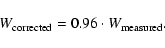
![$\displaystyle [{\rm Me/H}]_{\rm Stromgren}=-0.06+0.94~[{\rm Fe/H}]_{\rm Spectroscopic}$](/articles/aa/full/2005/34/aa2797-05/img64.gif)

![$\displaystyle -2.75 < {[\rm Fe/H]} < -1.0\!:$](/articles/aa/full/2005/34/aa2797-05/img136.gif)
![$\displaystyle \qquad{[\rm O/Fe]} =0.52-0.06~[{\rm Fe/H}], ~ \sigma_{\rm std}=0.12$](/articles/aa/full/2005/34/aa2797-05/img137.gif)
![$\displaystyle \qquad-1.0 < {[\rm Fe/H]} < 0.25\!:$](/articles/aa/full/2005/34/aa2797-05/img138.gif)
![$\displaystyle \qquad{[\rm O/Fe]} =0.00-0.60~{[\rm Fe/H]}, ~ \sigma_{\rm std}=0.12 ,$](/articles/aa/full/2005/34/aa2797-05/img139.gif)
![$\displaystyle \qquad{[\rm O/Fe]} =0.55-0.04~{[\rm Fe/H]}, ~ \sigma_{\rm std}=0.14$](/articles/aa/full/2005/34/aa2797-05/img141.gif)
![$\displaystyle \qquad{[\rm O/Fe]} =0.01-0.58~{[\rm Fe/H}], ~ \sigma_{\rm std}=0.12 .$](/articles/aa/full/2005/34/aa2797-05/img142.gif)